Article

Data-Driven Online Energy Scheduling of a Microgrid Based on Deep Reinforcement Learning

College of Information Science and Engineering, Northeastern University, Shenyang 110819, China
*
Author to whom correspondence should be addressed.
Energies 2021, 14(8), 2120; https://doi.org/10.3390/en14082120
Submission received: 13 March 2021 / Revised: 7 April 2021 / Accepted: 8 April 2021 / Published: 10 April 2021

Abstract

:
The proliferation of distributed renewable energy resources (RESs) poses major challenges to the operation of microgrids due to uncertainty. Traditional online scheduling approaches relying on accurate forecasts become difficult to implement due to the increase of uncertain RESs. Although several data-driven methods have been proposed recently to overcome the challenge, they generally suffer from a scalability issue due to the limited ability to optimize high-dimensional continuous control variables. To address these issues, we propose a data-driven online scheduling method for microgrid energy optimization based on continuous-control deep reinforcement learning (DRL). We formulate the online scheduling problem as a Markov decision process (MDP). The objective is to minimize the operating cost of the microgrid considering the uncertainty of RESs generation, load demand, and electricity prices. To learn the optimal scheduling strategy, a Gated Recurrent Unit (GRU)-based network is designed to extract temporal features of uncertainty and generate the optimal scheduling decisions in an end-to-end manner. To optimize the policy with high-dimensional and continuous actions, proximal policy optimization (PPO) is employed to train the neural network-based policy in a data-driven fashion. The proposed method does not require any forecasting information on the uncertainty or a prior knowledge of the physical model of the microgrid. Simulation results using realistic power system data of California Independent System Operator (CAISO) demonstrate the effectiveness of the proposed method.

1. Introduction

Microgrids have been widely adopted and deployed in modern power systems to improve energy efficiency and power supply security by integrating distributed energy resources [1]. According to statistics by BNResearch [2], there have been 6610 microgrid projects globally representing 31.7 GW of planned and installed power capacity by March 2020. The rapid deployment of microgrids brings many advantageous features, such as reducing long-distance transmission losses, decreasing the cost of the energy mix, and providing a new paradigm of energy infrastructure for future smart cities [3]. However, due to some special features in these small, self-governing systems, energy management of microgrids faces several major challenges. High proportional RES combined with stochastic load can lead to significant power variations and make it difficult to produce accurate generation schedules based on data forecasts. Moreover, microgrids contain various heterogeneous resources, such as energy storage systems (ESS) and dependent response resources, which cannot be dispatched according to the conventional unit-commitment and economic dispatch methods.
To overcome these challenges, extensive model-based online scheduling approaches have been proposed in the literature. For example, in [4], a rolling horizon optimization method based on mixed integer linear programming is proposed for energy management of a battery energy storage system. In [5], a model predictive control (MPC) method is proposed to optimize the operation of a renewable hydrogen-based microgrid with hybrid storage. In [6], an MPC based strategy combining two-stage stochastic programming considering the uncertainty of RES generation, system load, and electricity prices is designed. In [7], a chance-constrained MPC method is proposed and integrated into a hierarchical stochastic energy management system for operation management of interconnected microgrids. In [8], an MPC-based optimal energy management system is designed for the economic re-scheduling of a network of interconnected microgrids under failure conditions. In [9], a two-stage stochastic MPC strategy is developed to manage the local operation of individual microgrid in multi-microgrid systems. Besides, heuristic algorithms have also been used to solve the microgrid scheduling problem to avoid local optimum. For example, in [10], a non-dominated sorting genetic algorithm (GA) is developed to optimize the real-time energy management of a cyber physical multi-source energy system. In [11], a hierarchical GA optimization method is applied to a fuzzy logic-based energy management system considering the time-of-use energy price.
Although these methods have been successfully applied in the aforementioned and many other studies, they generally rely on an accurate forecast of the uncertainty, an explicit physical model of the microgrid system, and an efficient solver for the optimization model. Hence, to construct a model-based method, one needs specific domain knowledge on forecasting techniques, modeling methods, and solution algorithms. This may increase the implementation difficulty in real-world applications. In addition, to design an optimization model, precise system parameters and accurate forecasting information of uncertainty are necessary. These prerequisites may not be satisfied in some real-world scenarios, and the performance may deteriorate due to imprecise model parameters or inaccurate forecasts. It is worth mentioning that, although heuristic algorithms (e.g., [10,11]) are less dependent on physical models, they still require accurate forecasts to derive optimal scheduling decisions.
To reduce the dependency on accurate forecasting information and an explicit model, learning-based methods have been proposed in recent years. For instance, in [12], a batch RL algorithm is developed to optimize the ESS charging schedules in a microgrid. In [13], a Bayesian RL method and a dual-iterative Q-learning algorithm are applied for optimal operation of battery banks in multi-agent residential energy management system. In [14], an approximate dynamic programming (ADP) method is proposed for optimal control of ESSs considering the uncertainty of RES generation. In [15], an ADP-based algorithm is developed to learn the optimal energy management strategy of a grid-connected microgrid. In [16], an ADP method is used to integrate the ESS scheduling into conventional economic dispatch task for real-time microgrid energy management. In [17], an ADP-based stochastic nonlinear optimization approach is proposed for the real-time operation of the microgrid under uncertainties. In [18], a RL-based bi-level energy management system is proposed for optimal scheduling of networked microgrids under incomplete information. These methods generally use a linear or a simple nonlinear approximator to learn the value/action–value function and train the approximator through temporal difference learning.
Although these methods reduce the dependency on accurate forecasting information or an explicit physical model, the limited approximation capability hinders their application in real-world microgrid environments, which exhibit serious nonlinearity and uncertainty. With the development of deep learning technologies, many researchers have made efforts to develop DRL-based approaches for real-time energy scheduling of microgrids by taking advantage of the nonlinear representation capability of deep neural networks (DNNs). For example, in [19], a deep Q-learning (DQN) method is employed to solve the battery energy management problem and a convolutional neural network is designed to learn the optimal charging schedules using historical electricity prices. In [20], a constrained policy optimization method is used to learn the optimal electric vehicle (EV) charging strategy from historical electricity prices and user’s commute behavior. In [21], a double dueling DQN algorithm is adopted to learn the optimal battery control policy in a smart energy network. In [22], a DQN-based method is developed to solve the real-time energy management of microgrids considering the uncertainties of load demand, RES generation and electricity prices. In [23], a DRL algorithm using Monte Carlo Tree Search method is designed for online scheduling of a residential microgrid. In [24], a double-DQN based distributed operation strategy is proposed to optimize the online energy management of a community battery system in a microgrid considering uncertainty. In [25], an intelligent multi-microgrid energy management system is developed based on a model-free RL approach. A DNN is trained using the RL approach to manage the aggregated power exchange of the multi-microgrid system with the distribution system. In [26], DQN is applied to learn an optimal scheduling policy based on a convolutional neural network (CNN) for the operation of an isolated microgrid considering the penalty of non-served power.
However, the aforementioned methods can only handle discrete control actions and are not suitable for continuous ones. Therefore, to apply these methods to learn continuous control policies, the actions have to be discretized. Consequently, when the number of controllable devices increases or the granularity of the discretization becomes small, the number of actions will increase exponentially, which can make the problem intractable to solve. In addition, since the control actions for ESSs and distributed generators (DGs) are generally continuous in realistic microgrids, the performance of these methods may deteriorate due to the discretization of the action space. In the latest research [27], deep deterministic policy gradient (DDPG) has been applied to deal with continuous control variables in optimal scheduling of a microgrid. However, the scheme proposed in [27] still relies on accurate forecasts of future renewable generation and system load to make scheduling decisions.
In this paper, we propose a novel online scheduling method for microgrid energy management based on a continuous-control DRL algorithm. To reduce the dependency on accurate forecasts or an explicit physical model, we propose a data-driven formulation method based on MDP. To address the uncertainty of RES generation, system load, and electricity prices, we adopt a GRU network to extract their temporal features from historical data [28]. GRU is a variant of long shor-term memory (LSTM), which is effective in modeling long-term dependencies of sequential data. LSTM has been successfully applied in many applications of power and renewable energy systems, such as wind speed forecasting [29,30,31,32]. Compared to LSTM, GRU can achieve comparable performance with a simpler architecture and fewer tensor computations [33]. Based on the features extracted by GRU, a deep neural network architecture is designed to learn the optimal control policy in an end-to-end manner. The designed policy network can directly generate scheduling decisions without using any forecasting information or solving complex optimization models. To learn the optimal policy with continuous actions, a continuously-controlled DRL algorithm based on PPO [34] is employed to train the neural network based policy. Compared to the existing work, the main contributions of this work are summarized as follows:
  • To reduce the dependency on accurate forecasting information or an explicit physical model, we propose a data-driven formulation method for online energy scheduling of a microgrid based on MDP. This formulation enables us to optimize the scheduling decisions without having accurate forecasts of the uncertainty or knowing precise system model of the microgrid.
  • To avoid solving complex optimization problems during online scheduling, we design a GRU-based neural network to learn the optimal policy in an end-to-end fashion. During online execution of the scheduling policy, the neural network can directly produce scheduling decisions based on historical data and current state without predicting the uncertainty or solving complex optimization models.
  • To effectively learn the optimal scheduling policy for our problem with continuously-controlled devices, we employ the PPO algorithm to train the GRU-based policy network. The PPO-based method is effective for optimizing high-dimensional continuous-control actions and practical for real-world microgrid environments.
The rest of the paper is organized as follows. Section 2 formulates the problem. Section 3 presents the designed neural network and the DRL-based solution. Case studies are presented in Section 4. Section 5 draws the conclusions.

2. MDP Formulation of Online Energy Scheduling in Microgrids

Consider a microgrid with a set of DGs denoted by D = { 1 , 2 , , D } , a set of ESSs denoted by B = { 1 , 2 , , B } , a set of RESs denoted by R = { 1 , 2 , , R } , and a set of controllable loads denoted by L = { 1 , 2 , , L } . We assume that the microgrid operates in a grid-connected mode and participates in the real-time electricity market. We divide the intra-day operation into T time slots, indexed by { 1 , 2 , , T } , and the interval of two time slots is Δ t .
We formulate the online scheduling of a microgrid as an MDP with an unknown system model. The MDP is represented by a 5-tuple ( S , A , P a , R a , γ ) , where S is a set of the system states, A is a set of feasible actions, P a : S × A × S [ 0 , 1 ] is the state transition probability, R a : S × A R is the reward function, and γ [ 0 , 1 ) is the discount factor. In the following subsections, we present the states, actions, rewards, and objective of the MDP model in detail.

2.1. States

The state includes two kinds of information: (1) the historical data about the uncertainties, including the net load of the microgrid system and the electricity prices; and (2) the energy of the ESSs at the current time slot t. Thus, the state s t is defined by
s t = [ P L ( t T ) , , P L ( t 1 ) , ρ ( t T ) , , ρ ( t 1 ) , E 1 ESS ( t ) , , E B ESS ( t ) ] T ,
where P L ( t T ) , , P L ( t 1 ) are the net load in the past T time slots; ρ ( t T ) , , ρ ( t 1 ) are the electricity prices in the past T time slots; and E 1 ESS ( t ) , , E B ESS ( t ) are the energy stored in the ESSs at the beginning of the time slot t.
The net load P L ( τ ) in any time slot τ [ t T , t 1 ] is calculated by
P L ( τ ) = P UL ( τ ) + l L P l CL ( τ ) r R P r RES ( τ )
where P UL ( τ ) denotes the total power demand of the microgrid in time slot τ , P l CL ( τ ) is the power consumption of the lth controllable load in time slot τ , and P r RES ( τ ) denotes the power generation of the rth RES unit.

2.2. Actions

The controllable devices in a microgrid include dispatchable DGs, controllable loads, and ESSs. Thus, the action is defined by
a t = [ P 1 DG ( t ) , . . . , P D DG ( t ) , P 1 CL ( t ) , . . . , P L CL ( t ) , P 1 ESS ( t ) , . . . , P B ESS ( t ) ] T ,
where P 1 DG ( t ) , , P D DG ( t ) are the output power of the dispatchable DGs in time slot t; P 1 CL ( t ) , , P L CL ( t ) are the power consumption of the controllable loads in time slot t; and P 1 ESS ( t ) , , P B ESS ( t ) are the charging/discharging power of the ESSs in time slot t.
The feasible set of the action a t in time slot t is defined by A t = A t DG A t ESS A t CL , where
A t DG = d D { P d DG ( t ) | P ̲ d DG P d DG ( t ) P ¯ d DG } A t CL = l L { P l CL ( t ) | P ̲ l CL P l CL ( t ) P ¯ l CL } A t ESS = b B { P b ESS ( t ) | P ̲ b , t ESS P b ESS ( t ) P ¯ b , t ESS } .
Here, P ̲ d DG and P ¯ d DG represent the minimum and maximum output power of the DG d, respectively; P ̲ l CL and P ¯ l CL denote the minimum and maximum power demand of the controllable load l L ; and P ̲ b , t ESS and P ¯ b , t ESS denote the maximum discharging or charging power of the ESS b B in time slot t.
It is notable that maximum discharging or charging power P ̲ b , t ESS and P ¯ b , t ESS are time-variant due to the capacity constraint of the ESS. The maximum discharging or charging power can be calculated according to
P ̲ b , t ESS = min [ ( E b ESS ( t ) E ̲ b ESS ) η b d c h / Δ t , P ¯ b ESS ] P ¯ b , t ESS = min [ ( E ¯ b ESS E b ESS ( t ) ) / η b c h Δ t , P ¯ b ESS ]
where P ¯ b ESS is the rated power of the ESS b; E b ESS ( t ) denotes the energy stored in the ESS at the beginning of the time slot t; E ̲ b ESS , and E ¯ b ESS are the allowable minimum and maximum energy stored in the ESS, respectively; and η b c h and η b d c h are the charging and discharging efficiency, respectively.

2.3. Rewards

To minimize the operational cost of the microgrid and guarantee the power balance between supply and demand, we define the reward r t in time slot t as the negative operational cost plus a penalty term:
r t = d D C d DG ( t ) + l L C l CL ( t ) + C G ( t ) ω · max ( | P G ( t ) | P ¯ G , 0 )
where C d DG ( t ) denotes the fuel cost of the DG d in time slot t, C l CL ( t ) denotes the curtailment cost of CL l in time slot t, C G ( t ) represents the transaction cost with the utility grid, and max ( | P G ( t ) | P ¯ G , 0 ) is the penalty term.
The fuel cost of the DG d in time slot t is calculated by a quadratic function of the output power P d DG ( t ) [15]:
C d DG ( t ) = [ a d P d DG ( t ) 2 + b d P d DG ( t ) + c d ] Δ t ,
where a d , b d , and c d are the cost coefficients of the DG d.
The curtailment cost of the controllable load l is calculated by the following quadratic function [35]
C l CL ( t ) = β l P ¯ l CL P l CL ( t ) 2
where β l is a positive coefficient, reflecting the customer’s sensitivity to load curtailment.
The transaction cost with the utility grid is calculated by,
C G ( t ) = ρ ( t ) · P G ( t ) Δ t , if P G ( t ) 0 α ρ ( t ) · P G ( t ) Δ t , otherwise .
where P g ( t ) denotes the power exchanged with the main grid in time slot t. In our study, the microgrid participates in the real-time electricity market and is charged with the real-time locational marginal price (LMP). To encourage local utilization of RESs, we assume that the selling prices are lower than the purchasing prices, i.e., α ρ ( t ) , where 0 < α < 1 is a discount.
The penalty term max ( | P G ( t ) | P ¯ G , 0 ) measures the power imbalance between supply and demand. The penalty term is greater than 0 when the absolute value of the power imported from the utility grid or the power exported to the utility grid exceeds the maximum capacity, i.e., | P G ( t ) | P ¯ G .

2.4. Objective Function

We aim to find a scheduling policy π ( a t | s t ) : s t a t to maximize the total expected rewards over the scheduling horizon T. Thus, the objective is defined as
max π Π J ( π ) = E τ π t = 0 T 1 γ t · r t
where E τ π [ · ] denotes the expected value over the trajectory τ = ( s 0 , a 0 , s 1 , , a T 1 , s T ) ; τ π is shorthand for indicating that the distribution over the trajectory τ depends on the policy π : a t π ( · | s t ) , s t + 1 P a ( · | s t , a t ) , and P a ( · | s t , a t ) is the state transition probability given a t at the state s t ; γ [ 0 , 1 ) is the discount factor, which determines how much we care about rewards in the distant future relative to those in the immediate future; and r t R is the reward received at the time slot t, which is defined in Equation (6), representing the negative of the operational cost of the microgrid and the penalty for power imbalance.

3. Deep Reinforcement Learning Solution Based on Proximal Policy Optimization

The MDP formulation of the microgrid real-time energy scheduling problem has multiple continuous actions. This problem is challenging for many DRL algorithms because of the large and continuous action space. To solve this issue, we employ the PPO algorithm, which has been successful at solving high-dimensional continuous control problems [34,36]. Besides, we design a deep neural network to learn the optimal policy, which can directly output the scheduling decisions based on the microgrid states and the historical data of the uncertainties.

3.1. Proximal Policy Optimization Algorithm

For the MDP formulation, we aim to find the optimal control policy π ( a t | s t ) maximizing the objective J ( π ) . However, this problem is difficult to solve because the policy π ( a t | s t ) is a function of state s t . To approach this problem, we consider a parameterized policy π θ ( a | s ) , which depends on the parameter vector θ . Now, instead of directly optimizing the policy π ( a t | s t ) , we are interested in optimizing the parameter θ * in the space Θ such that
θ * = arg max θ Θ J ( θ ) ,
where we replace J ( π ) with J ( θ ) because we are considering a parameterized policy π θ ( a | s ) . In the following, we replace all functions of notation π with functions of θ for brevity.
PPO is an efficient local policy search method for MDP problems. In traditional local policy search methods, such as trust-region policy optimization (TRPO) [37], the policy parameter θ is iteratively updated by optimizing a surrogate function of the objective J ( θ ) in the neighborhood of the most recent iterate θ i
max θ Θ E s ρ , a π θ π θ ( a | s ) π θ i ( a | s ) A θ i ( s , a ) s . t . D KL max ( θ i | | θ ) δ
where ρ denotes the discounted expected distribution of the state s, A θ i ( s , a ) represents the advantage function, and D KL max ( θ i | | θ ) = max s D KL ( π θ i ( · | s ) | | π θ ( · | s ) ) is the maximum KL divergence with respect to s. The KL-divergence D KL max ( θ i | | θ ) defines the searching area in the neighborhood of θ i . However, this method is a second-order algorithm and is computationally expensive. This is because it requires calculating the inverse of a Hessian matrix to estimate the KL-Divergence D KL max ( θ i | | θ ) and solving the nonlinear constrained optimization problem (12).
To improve the computational efficiency, PPO converts this problem to a unconstrained optimization problem by heuristically restricting the likelihood ratio
r ( θ ) = π θ ( a | s ) π θ i ( a | s )
as a penalty in the objective instead of confining the KL-Divergence D KL max ( θ i | | θ ) in the constraint. Specifically, PPO updates the parameter θ by iteratively solving the following
θ i + 1 = arg max θ Θ L θ i ( θ ) L θ i ( θ ) = E t min r t ( θ ) A ^ θ i t , CLIP r t ( θ ) , 1 ϵ , 1 + ϵ A ^ θ i t .
where CLIP ( r t ( θ ) , 1 ϵ , 1 + ϵ ) means clipping the likelihood ratio r t ( θ ) by the boundaries 1 ϵ and 1 + ϵ and ϵ is a hyperparameter. A ^ θ i t is an estimator of the advantage function A θ i ( s , a ) , which can be calculated by [38]:
A ^ θ i t = δ t + ( λ γ ) δ t + 1 + + ( λ γ ) T t 1 δ T 1 δ t = r t + V θ i ( s t ) V θ i ( s t + 1 ) .
where λ [ 0 , 1 ] is the generalized advantage estimation parameter, γ [ 0 , 1 ) is the discount factor, and V θ i ( s t ) = E s t , a t , s t + 1 , . . . [ l = 0 γ l r t + l ] denotes the value function under the policy π θ i .
Note that the PPO policy update rule (14) can be solved by using a first-order gradient descent algorithm. This means that we no longer need to estimate the KL divergence or solve a nonlinear constrained optimization problem. Thus, the PPO algorithm is more computationally efficient than TRPO.

3.2. Design of the Policy and Value Network

In our study, we use a deep neural network to learn the policy π θ ( a t | s t ) as well as the value function V θ ( s t ) . Note that the neural network is designed in an end-to-end fashion, which means that we do not require any hand-crafted features. The overall architecture of the designed network is illustrated in Figure 1. The network consists of three parts: a gated recurrent network, a feed-forward network, and an output layer. The gated recurrent network is used to extract time-series features from historical data on the net load and electricity prices. The feed-forward network concatenates the time-series features as well as the current system state and outputs high-level features. The output layer is used to predict the state value and generate control decisions. Next, we explain the overall design in details.
Knowing the future trend of the uncertainties, i.e., the system net load and electricity prices, is crucial to the learning of the policy and the value function. Since the load and electricity prices generally fluctuate in a quasi-periodic way, it is reasonable to infer the future trend from their past realizations. In our study, we employ GRU [39] to extract the future trend features.
GRU is a variant of long-short term memory (LSTM), which is effective in modeling long-term dependencies of sequential data [28]. Compared to traditional recurrent neural networks (RNNs), LSTM networks utilize gates and the cell state to extract and carry relevant information throughout the processing of sequential data. This mechanism makes it possible to preserve information from very early time steps and build connection to one extracted from later time steps. Therefore, LSTM networks are very suitable for time-series data modeling. However, LSTM networks are more computationally complex than traditional RNNs are.
GRU improves the LSTM model by removing the cell state and uses the hidden state to carry information. Compared to LSTM, GRU has fewer gates and tensor operations; therefore, GRU can be trained slightly more quickly than LSTM. GRU networks have also been successfully applied in many smart grid applications, such as load forecasting [40] and wind power prediction [41].
In our design, the GRU network takes as inputs the net load and electricity prices of the past T time slots and outputs the features about their future trends. The features extracted by the GRU and the energy in all ESSs, E 1 ESS ( t ) , , E B ESS ( t ) , are then concatenated together as a vector, which is inputted into the feed-forward network. The feed-forward network transforms the inputs into high-level features by passing them through two hidden layers of 128 rectified linear unit (ReLU) neurons:
f l = max ( W l f l 1 + b l , 0 ) , l = 1 , 2
where f l is the output feature of the lth layer and W l and b l are the weights and biases of the lth layer, respectively.
The output layer uses the features extracted by the feed-forward network to approximate the policy and the value function. Specifically, since the control variables are continuous in our formulation, we define the stochastic policy by the normal distribution π θ ( a | s ) N ( μ , Σ ) , where the mean μ and covariance Σ are approximated by:
μ = W μ f L + b μ , D i a g ( Σ ) = b σ ,
where f L , L = 2 denotes the latent features extracted by the feed-forward network. W μ , b μ , b σ are the weights and biases of the output layer, respectively. Note that the covariance Σ is defined as a diagonal matrix and only the elements of the principal diagonal are approximated. When executing the policy, actions are sampled according to the normal distribution approximated by the neural network.
In addition, the value function is approximated by
V θ ( s ) = W o f L + b o
where W o and b o are the weights and biases of the output layer with respect to the value function.

3.3. Practical Implementation

In the practical implementation, we train the overall network based on a sample-based procedure. Specifically, at iteration i, we simulate the policy π θ i in a microgrid simulation environment for a certain amount of time steps, e.g. N × T . We record the simulation trajectory τ = { s 0 , a 0 , r 0 , , s T } 1 , , N . Then, we use the trajectory data to calculate the sampled values of the advantage function according to Equation (15) and the sample probability π θ i ( a t | s t ) . Then, we optimize the parameter vector θ by maximizing the augmented PPO objective:
L ¯ θ i ( θ ) = L θ i ( θ ) + κ 1 E t ( V θ ( s t ) V t targ ) 2 + κ 2 E t S [ π θ ] ( s t )
where the term ( V θ ( s t ) V t targ ) 2 is the square error of the approximate value function and the term E t S [ π θ ] ( s t ) represents the entropy bonus, which ensures sufficient exploration, as suggested by Volodymyr [42]. κ 1 and κ 2 are coefficients. The pseudo-code of the PPO algorithm is summarized in Algorithm 1.
Algorithm 1 The PPO algorithm for microgrid real-time scheduling
  • Initialize network parameter θ 0 .
  • for i = 1 , 2 , do
  • for n = 1 , 2 , , N do
  •   Initialize the microgrid state s 0
  •   for t = 0 , 1 , , T 1 do
  •    Select action a t according to the policy π θ i ( a t | s t )
  •    Check safety of a t and simulate the environment
  •    Store transition ( s t , a t , r t ) in τ
  •   end for
  •   Calculate A ^ θ i t and V t targ for t = 0 , 1 , T 1
  • end for
  •  Set θ 0 i : = θ i
  • for k = 0 , 1 , , K 1 do
  •   Optimizing L ¯ θ k i ( θ ) with minibatch size M N T
  •   Set θ k + 1 i : = arg max θ L ¯ θ k i ( θ )
  •   Set θ i + 1 : = θ K i
  • end for
  • end for

4. Case Studies

4.1. Experimental Setup

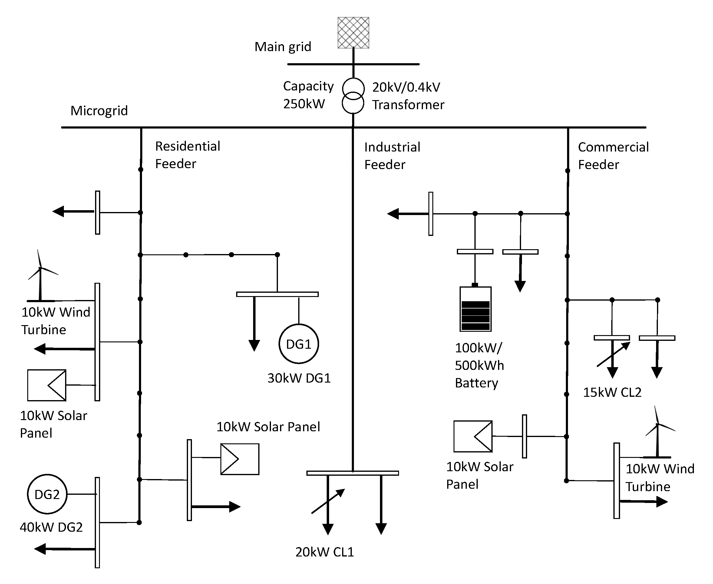
We evaluate the proposed method in the CIGRE benchmark microgrid system [43] (Figure 2). The microgrid contains two dispatchable DGs with capacities of 30 and 40 kW; one battery ESS with a capacity of 500 kWh and a maximum charging/discharging power of 100 kW; three solar panel generators and two wind turbines with a capacity of 10 kW each; two controllable loads; and some uncontrollable loads. The maximum exchange power between the microgrid and utility grid is 300 kW. Other parameters of the controllable devices are summarized in Table 1.
To simulate the uncertainties, we use realistic power system data from CAISO [44]. The data include wind and solar generation, load demand, and electricity prices with a period of one year in 2019 and a resolution of 1 h. To consider the weekly load profile or seasonal change of weather, we use the first three weeks of each month as the training set and the remaining data as the testing set. To encourage local utilization of RESs, we assume the selling prices are 20% lower than the purchasing prices.
For the policy and value network, we use 24 GRUs to extract a 128-dimension feature vector from the past 24 h’ net loads and electricity prices. This feature vector is concatenated with the energy of the ESS at time interval t as the input of the feed-forward neural network. The feed-forward neural network has two hidden layers of 128 ReLU neurons. The output layer outputs a five-dimensional vector, which approximates the means μ of the stochastic policy π θ ( a | s ) N ( μ , Σ ) . The neural network weights are randomly initialized by using the orthogonal initialization technique and updated by the Adam optimization [45] during the training process. Other parameters used in the algorithm are summarized in Table 2. The microgrid environment is established by using the power system simulation package PYPOWER [46] and the DRL environment package GYM. The algorithm was coded in Python using the neural network Toolbox 2.2.0 Tensorflow and RL Toolbox Baselines-tf2. The program was run in the Ubuntu system on an 8-core i7-6700K CPU.

4.2. Comparison with Commonly Used Online Scheduling Methods

To validate the proposed approach, we train the GRU-based network model using the training set and then evaluate the well-trained model on the testing set. To demonstrate the advantages of the proposed approach, we compare it with three commonly used online scheduling methods: (1) MPC; (2) ADP; and (3) GA. (1) MPC is a widely used model-based online scheduling method [5,6,7,8,9], which addresses the uncertainty via rolling/receding horizon optimization. At each time step, a multi-timestep optimization model is solved based on real-time forecasts over a prediction horizon. Then, the optimal solution at the first time step is implemented as the present scheduling decisions. In the experiment, the window size is set to 8 and the forecasting data are generated by adding the actual value to a forecasting error. The forecasting error is sampled from a normal distribution N ( 0 ; δ 2 ) , where the standard deviation is set to be 15% of the actual value of the uncertainty. (2) ADP is commonly-used RL approach [15,16,17], which models the online scheduling problem as a dynamic programming. To overcome the “curse of dimensionality”, ADP uses an approximate value function (AVF) to solve the Bellman equation to derive the near-optimal online scheduling decisions. In the experiment, we use an M × T lookup table [17] to approximate the value function, where M is the size of the reduced state space. To avoid an extremely large lookup table, we use the method in [17] to reduce the state space. Specifically, we exclude the historical electricity price and net load from the state s t , and discretize the remaining continuous state variables, i.e., s ̲ t = [ ρ ( t 1 ) , P L ( t 1 ) , E 1 ESS ( t ) ] , into M = 10 × 10 × 10 = 1000 distinct states. The temporal difference error algorithm is used to update the table. (3) GA is a heuristic optimization method, which has been used to solve microgrid scheduling problems [10,11]. To apply GA to the online scheduling of a microgrid, we combine it with MPC by implementing a rolling horizon optimization. In the experiment, the sliding window and the forecasting data are set to be the same as those used in MPC. Different from MPC; however, we solve the multi-timestep optimization model at each time step by using GA instead of the commercial optimization solver Gurobi [47]. The parameter setting of the GA algorithm is as follows: population size, 100; mutation probability, 0.1; crossover rate, 0.5; parents portion, 0.3; and number of generations, 500.
We compare the proposed approach with the commonly used methods in the following aspects:
(a) Total operating cost: The testing set contains 113 testing days and the operating cost of each testing day is calculated according to
F = t = 0 T 1 d D C d DG ( t ) + l L C l CL ( t ) + C G ( t )
where C d DG ( t ) , C l CL ( t ) , and C G ( t ) are defined in Equations (7)–(9), respectively.
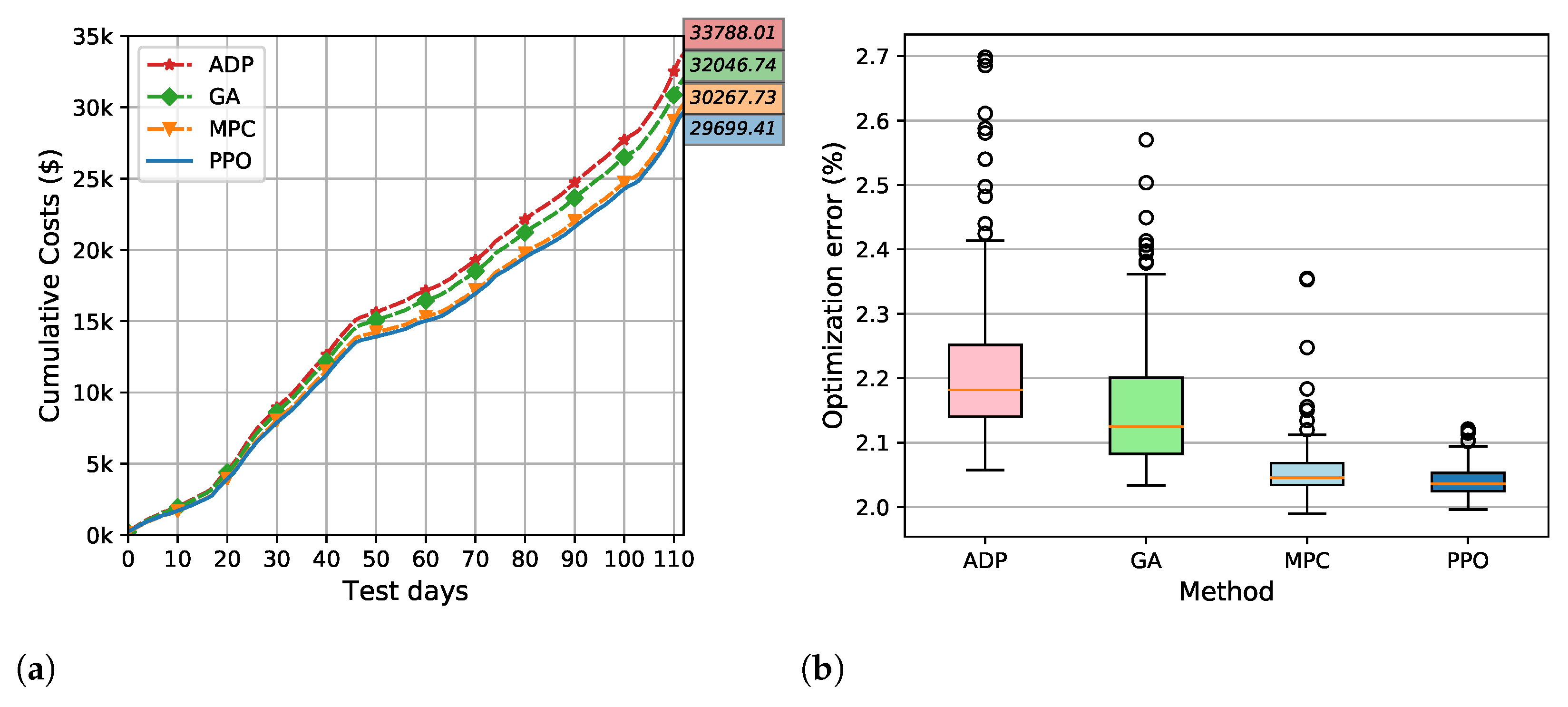
Figure 3a compares the cumulative operating costs on 113 testing days obtained by ADP, GA, MPC, and the proposed approach (PPO). It can be observed that the proposed approach obtains the best total operating cost, i.e., $29,699.41, which is 7.32% lower than that of GA ($32,046.74), 12.10% lower than that of ADP ($33,788.01), and 1.877% lower than that of MPC ($30,267.73). Among these methods, ADP performs the worst. This is because the discretization of the state space limits its ability to accurately approximate the value function, resulting in sub-optimal scheduling decisions. GA and MPC both perform better than ADP since they use real-time forecasting information to adjust the scheduling decisions. However, GA does not perform as well as MPC does. This is because the commercial solver Gurobi used in MPC can find the global optimum (duality gap is 0). In addition, MPC performs almost as well as PPO does, but its performance is affected by the prediction error, and thus inferior to that of the proposed approach. Furthermore, compared to these methods, the proposed approach does not need any forecasts on the uncertainty or efforts on solving an optimization model.
(b) Optimization error: The optimization error is defined as the performance gap between an online scheduling approach and “Theoretical Optimum”. The Theoretical Optimum assumes that the uncertainty can be accurately predicted. Using the accurate prediction, the Theoretical Optimum models the problem as a mixed integer quadratic programming (MIQP) and solves for the optimal solution via Gurobi. The optimization error is calculated by
E R R o n l i n e = F o n l i n e F T O F T O × 100 %
where F o n l i n e and F T O represent the daily operating cost (20) obtained by the online scheduling approaches (MPC, ADP, GA, and PPO) and the Theoretical Optimum, respectively.
Since the Theoretical Optimum uses perfect forecasting information, the optimization error can reflect the robustness of an online scheduling algorithm against uncertainty. Figure 3b compares the distribution of the optimization errors on the 113 testing days. It can be observed in the boxplot (Figure 3b) that, compared to MPC, ADP, and GA, the proposed approach (PPO) obtains the smallest optimization error in terms of first quartile (Q1), median, third quartile (Q2), and maximum. Moreover, the optimization errors of the proposed approach are more tightly grouped and have fewer outliers. This means that the proposed approach is less susceptible to the uncertainty on different testing days than the benchmarks are. This result demonstrates the superiority of the proposed approach over MPC, ADP, and GA in robustness.
(c) Online execution time: Table 3 compares the computation time at each time step during the online execution of each scheduling algorithm. It can be observed that the online execution time of ADP, GA, and MPC is much more than that of the proposed approach. This is because ADP, GA, and MPC all need to solve an optimization model during online scheduling whereas the proposed approach can directly generate the scheduling decision by the well-trained neural network. Among the commonly used methods, GA takes the most time, whereas ADP takes the least one. This is expected because ADP only needs to solve a one-step optimization problem but GA and MPC have to solve a multi-period optimization model. Besides, GA generally requires a population of candidate solutions to evolve many generations; therefore it takes more time than MPC does.
It is worth mentioning that the proposed approach needs about 11.5 h to train the GRU-based network. However, the training process can be performed offline. Once the offline training process is finished, we can implement it online to directly generate real-time scheduling decisions without forecasting the uncertainty or solving a complex optimization problem. The online execution time only takes about 0.5 ms on average.

4.3. Comparison with DQN

DQN is a well-known DRL approach, which has been used to solve the online scheduling problem in the latest research [22,24,26]. However, DQN can only handle discrete actions and suffers some limitations in solving our problem with continuously controlled devices, such as DGs, ESS, and controllable loads. To demonstrate the advantage of the proposed approach on handling continuous actions, we compare it with DQN. To apply DQN, we discretize the actions ( P 1 DG , P 2 DG , P 1 ESS , P 1 CL , P 2 CL ) into 2 × 2 × 2 × 2 × 2 = 32 choices, which consist of { P ̲ 1 DG , P ¯ 1 DG } { P ̲ 2 DG , P ¯ 2 DG } { P ̲ 1 , t ESS , P ¯ 1 , t ESS } { P ̲ 1 CL , P ¯ 1 CL } { P ̲ 2 CL , P ¯ 2 CL } . It is notable that, when the discretization granularity gets small, the number of actions increases exponentially, e.g., 4 × 4 × 4 × 4 × 4 = 1024 .
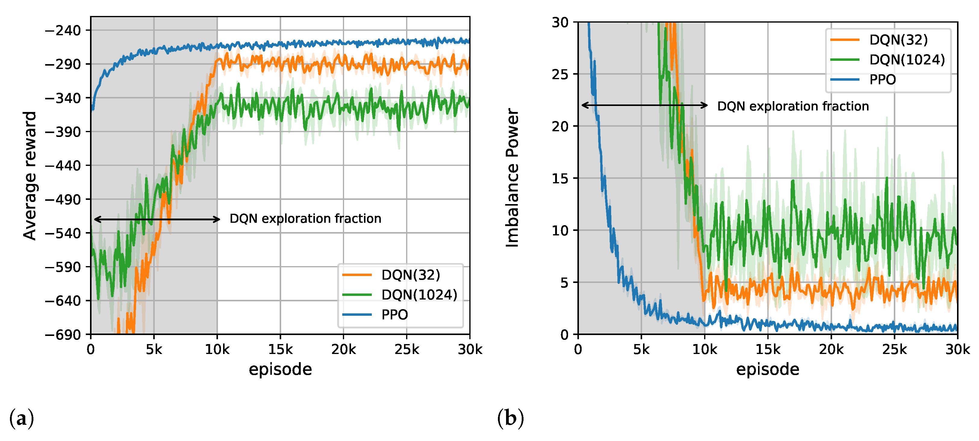
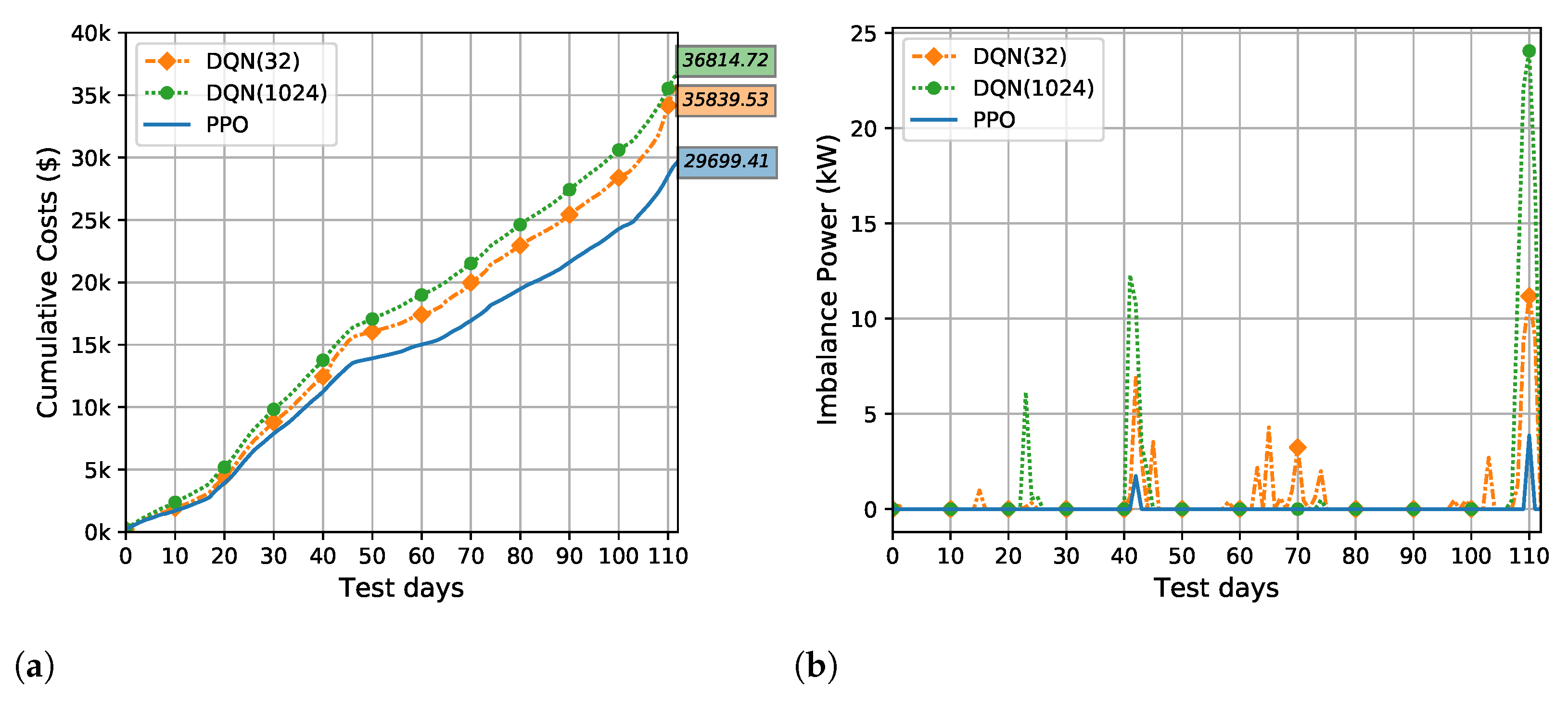
The training and testing performances are compared in Figure 4 and Figure 5, respectively. One observation from the comparison results is that the proposed method outperforms DQN during both the training and the testing processes. For the training performance, as shown in Figure 4a, the proposed method achieves the highest reward around 250 , whereas DQN only obtains a reward of 290 with 32 actions and 340 with 1024 actions. In addition, as shown in Figure 4b, the proposed method effectively restricts the imbalance power to a very small level below 1, whereas DQN causes a large imbalance in the range of 2.5 to 15. This means that DQN cannot guarantee that the power balance constraint is adequately satisfied. For the testing performance, as shown in Figure 5a, the proposed approach reduces the total operating cost by 17.13% and 31.12%, respectively, compared to the DQN methods with 32 actions and 1024 actions, respectively. Moreover, Figure 5b shows that, on some testing days, the DQN methods can cause very large power imbalance, which is rarely seen in the proposed approach. These comparison results demonstrate the advantage of the proposed method over the DQN method.
Another observation is that, for the DQN method, when the number of discretized actions increases (from 32 to 1024), the training and testing performance degrades. This is because, when the number of actions is large, it becomes difficult for the DQN method to balance between exploring novel actions that are not previously selected and exploiting actions that have worked well so far. Therefore, although discretizing the action space with a finer granularity gives a better approximation to the original continuous action space, it increases difficulties in the training process of the DQN-based method. However, the proposed method can directly handle continuously-controlled RL problems without discretization, and thus it is more suitable and practical for the online scheduling problem of microgrids.

4.4. Comparison with Other Continuously-Controlled DRL Methods

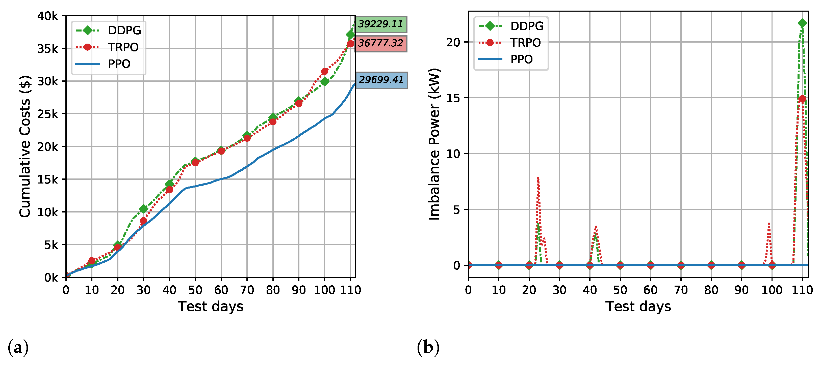
To further demonstrate the advantage of the proposed approach, we also compare with another two continuously-controlled DRL methods, DDPG and TRPO. The training and testing performances are compared in Figure 6 and Figure 7, respectively.
From the comparison results, we can observe that, although DDPG and TRPO can also handle continuous actions, the proposed approach outperforms them with a large margin, in terms of both the training and the testing performance. For example, compared to DDPG and TRPO, the proposed approach reduces the total operating cost on the testing set by 24.24% and 19.24%, respectively. Besides, the proposed approach can effectively manage the power supply and demand balance, whereas DDPG and TRPO fail to do so, resulting in some power imbalance in both the training and testing stages.
In terms of learning speed, DDPG shows a faster learning speed at the beginning of the training. This is because DDPG is an off-policy method, which can reuse past data samples to accelerate training. However, DDPG suffers from the stabilization issue due to the interplay between the deterministic actor network and the Q-function [36]. This issue clearly shows up in Figure 6, in which the performance of DDPG improves quickly at the beginning of the training but then deteriorates as the training goes from episodes 10k to 30k. In addition, the learning speed of TRPO is slower than that of the proposed approach and DDPG because TRPO requires numerous samples to estimate the KL-divergence D KL max ( θ i | | θ ) at each iteration. These comparison results demonstrate the advantages of the proposed approach over DDPG and TRPO in terms of learning speed, stability, and the final performance.

4.5. Scheduling Results

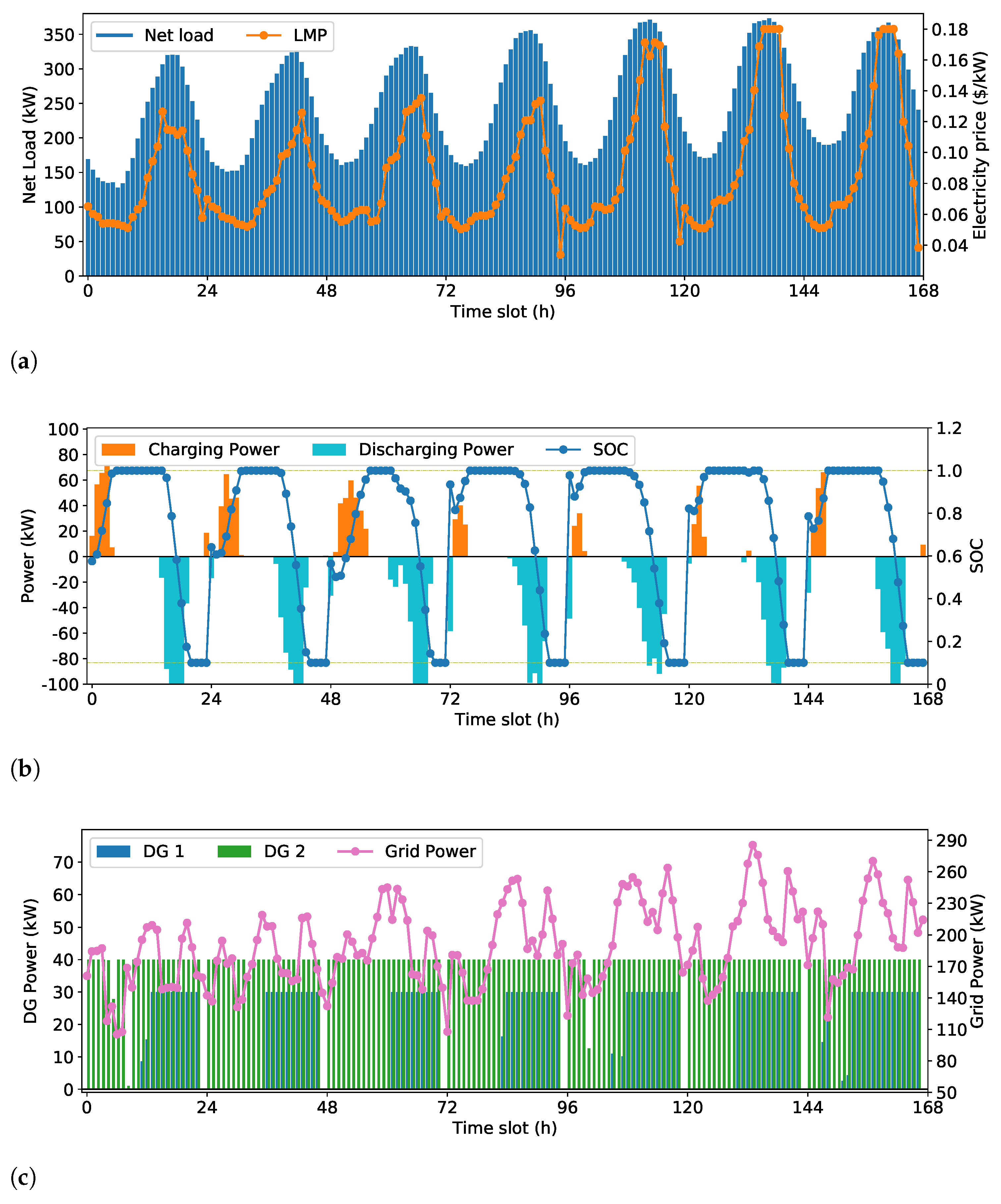
To validate the effectiveness of the decisions made by the proposed approach, the scheduling results on seven consecutive testing days are presented in Figure 8, which includes the charging/discharging power and state-of-charge (SOC) pattern of the battery, the power output of the DGs, the exchanged power between the microgrid and utility grid, and the power curtailment of the CLs. Figure 8b shows that the proposed method has successfully learned to charge the battery when the electricity prices are low and discharge it when the prices are at the peaks. In addition, Figure 8c shows that DG 1 is scheduled to operate with its maximum power output during peak-price hours in order to reduce the energy cost and stop operating when the prices are off the peaks. In addition, DG 2 is scheduled to operate with its maximum power most of the time because its cost is lower than that of buying from the utility grid. For both of the controllable loads, as shown in Figure 8d, when the prices are at the peaks, the power consumption is fully curtailed to reduce the operational cost. These results indicate that the proposed approach is effective in learning a cost-saving strategy to efficiently operate the microgrid.

5. Conclusions

We proposed a continuous-control DRL-based method for online energy scheduling of a microgrid. We formulated the online energy scheduling problem as an MDP with an unknown system model. To learn the optimal scheduling policy, we designed a GRU-based neural network to extract time-series features from historical data of the uncertainty. The GRU-based network can also directly output continuous scheduling decisions based on the microgrid state information and the extracted time-series features. Since the problem contains high-dimensional continuous control actions, the PPO algorithm was employed to train the neural network. We showed that the proposed method can learn a superior control policy for the online energy scheduling problem without requiring an accurate forecast model or prior knowledge of the physical model. Simulation results demonstrate that the proposed approach outperforms state-of-the-art DRL-based methods, including DDPG, TRPO, and DQN. Besides, the proposed method achieved a final performance in close proximity to the one obtained by the MIQP method under perfect information.

Author Contributions

Conceptualization, Y.J. and J.W.; methodology, Y.J.; software, Y.J.; validation, Y.J., and J.X.; formal analysis, Y.J., and J.X.; resources, J.X.; writing—original draft preparation, Y.J.; writing—review and editing, Y.J. and D.L.; supervision, J.W.; and project administration, J.W. All authors have read and agreed to the published version of the manuscript.

Funding

This research was funded by National Science Foundation of China grant number 61733003.

Institutional Review Board Statement

Not applicable.

Informed Consent Statement

Not applicable.

Data Availability Statement

http://oasis.caiso.com/mrioasis/logon.do (accessed on 10 August 2020).

Conflicts of Interest

The authors declare no conflict of interest.

Abbreviations

The following abbreviations are used in this manuscript:
ADPApproximate dynamic programming
CAISOCalifornia Independent System Operator
CLControllable load
DQNDeep Q-network
DDPGDeep deterministic policy gradient
DRLDeep reinforcement learning
DGDistributed Generator
ESSEnergy Storage System
GAGenetic Algorithm
GRUGated Recurrent Unit
LMPLocational marginal price
MDPMarkov decision process
MIQPMixed Integer Quadratic Programming
MPCModel Predictive Control
PPOProximal policy optimization
SOCState of Charge
TRPOTrust region policy optimization
RESRenewable energy resources
ReLURectified linear unit

References

  1. Huang, B.; Liu, L.; Li, Y.; Zhang, H. Distributed Optimal Energy Management for Microgrids in the Presence of Time-Varying Communication Delays. IEEE Access 2019, 7, 83702–83712. [Google Scholar] [CrossRef]
  2. BN Research. Projects and trends in the global microgrid market by region, segment, business model, and top states and countries. Navig. Res. Microgrid Deploy. Tracker 2020, 1Q20. Available online: https://guidehouseinsights.com/reports/microgrid-deployment-tracker-1q20 (accessed on 11 November 2020).
  3. Kazerani, M.; Tehrani, K. Grid of Hybrid AC/DC Microgrids: A New Paradigm for Smart City of Tomorrow. In Proceedings of the IEEE 15th International Conference of System of Systems Engineering (SoSE), Budapest, Hungary, 2–4 June 2020; pp. 175–180. [Google Scholar]
  4. Valencia, F.; Collado, J.; Sáez, D.; Marín, L.G. Robust Energy Management System for a Microgrid Based on a Fuzzy Prediction Interval Model. IEEE Trans. Smart Grid 2016, 7, 1486–1494. [Google Scholar] [CrossRef]
  5. Garcia-Torres, F.; Bordons, C. Optimal economical schedule of hydrogen-based microgrids with hybrid storage using model predictive control. IEEE Trans. Ind. Electron. 2015, 62, 5195–5207. [Google Scholar] [CrossRef]
  6. Li, Z.; Zang, C.; Zeng, P.; Yu, H. Combined Two-Stage Stochastic Programming and Receding Horizon Control Strategy for Microgrid Energy Management Considering Uncertainty. Energies 2016, 7, 499. [Google Scholar] [CrossRef] [Green Version]
  7. Bazmohammadi, N.; Tahsiri, A.; Anvari-Moghaddam, A.; Guerrero, J.M. A hierarchical energy management strategy for interconnected microgrids considering uncertainty. Int. J. Electr. Power Energy Syst. 2019, 109, 597–608. [Google Scholar] [CrossRef]
  8. Garcia-Torres, F.; Bordons, C.; Tobajas, J.; Marquez, J.J.; Garrido-Zafra, J.; Moreno-Munoz, A. Optimal Schedule for Networked Microgrids under Deregulated Power Market Environment using Model Predictive Control. IEEE Trans. Smart Grid 2020, 12, 182–191. [Google Scholar] [CrossRef]
  9. Bazmohammadi, N.; Anvari-Moghaddam, A.; Tahsiri, A.; Madary, A.; Vasquez, J.C.; Guerrero, J.M. Stochastic predictive energy management of multi-microgrid systems. Appl. Sci. 2020, 10, 4833. [Google Scholar] [CrossRef]
  10. Tehrani, K. A smart cyber physical multi-source energy system for an electric vehicle prototype. J. Syst. Archit. 2020, 111, 1383–7621. [Google Scholar] [CrossRef]
  11. Leonori, S.; Paschero, M.; Mascioli, F.M.F.; Rizzi, A. Optimization strategies for Microgrid energy management systems by Genetic Algorithms. Appl. Soft Comput. 2020, 86, 1568–4946. [Google Scholar] [CrossRef]
  12. Mbuwir, B.V.; Ruelens, F.; Spiessens, F.; Deconinc, G. Battery Energy Management in a Microgrid Using Batch Reinforcement Learning. Energies 2017, 10, 1846. [Google Scholar] [CrossRef] [Green Version]
  13. Anvari-Moghaddam, A.; Rahimi-Kian, A.; Mirian, M.S.; Guerrero, J.M. A multi-agent based energy management solution for integrated buildings and microgrid system. Appl. Energy 2017, 203, 41–56. [Google Scholar] [CrossRef] [Green Version]
  14. Wei, Q.; Shi, G.; Song, R.; Liu, Y. Adaptive Dynamic Programming-Based Optimal Control Scheme for Energy Storage Systems With Solar Renewable Energy. IEEE Trans. Ind. Electron. 2017, 64, 5468–5478. [Google Scholar] [CrossRef]
  15. Zeng, P.; Li, H.; He, H.; Li, S. Dynamic Energy Management of a Microgrid Using Approximate Dynamic Programming and Deep Recurrent Neural Network Learning. IEEE Trans. Smart Grid 2019, 10, 4435–4445. [Google Scholar] [CrossRef] [Green Version]
  16. Shuai, H.; Fang, J.; Ai, X.; Tang, Y.; Wen, J.; He, H. Stochastic Optimization of Economic Dispatch for Microgrid Based on Approximate Dynamic Programming. IEEE Trans. Smart Grid 2019, 10, 2440–2452. [Google Scholar] [CrossRef] [Green Version]
  17. Shuai, H.; Fang, J.; Ai, X.; Wen, J.; He, H. Optimal Real-Time Operation Strategy for Microgrid: An ADP-Based Stochastic Nonlinear Optimization Approach. IEEE Trans. Sustain. Energy 2019, 10, 931–942. [Google Scholar] [CrossRef] [Green Version]
  18. Zhang, Q.; Dehghanpour, K.; Wang, Z.; Huang, Q. A Learning-Based Power Management Method for Networked Microgrids Under Incomplete Information. IEEE Trans. Smart Grid 2020, 11, 1193–1204. [Google Scholar] [CrossRef] [Green Version]
  19. Cao, J.; Harrold, D.; Fan, Z.; Morstyn, T.; Healey, D.; Li, K. Deep Reinforcement Learning-Based Energy Storage Arbitrage With Accurate Lithium-Ion Battery Degradation Model. IEEE Trans. Smart Grid 2020, 11, 4513–4521. [Google Scholar] [CrossRef]
  20. Li, H.; Wan, Z.; He, H. Constrained EV Charging Scheduling Based on Safe Deep Reinforcement Learning. IEEE Trans. Smart Grid 2020, 11, 2427–2439. [Google Scholar] [CrossRef]
  21. Harrold, D.J.B.; Cao, J.; Fan, Z. Battery Control in a Smart Energy Network using Double Dueling Deep Q-Networks. In Proceedings of the 2020 IEEE PES Innovative Smart Grid Technologies Europe (ISGT-Europe), The Hague, The Netherlands, 26–28 October 2020; pp. 106–110. [Google Scholar]
  22. Ji, Y.; Wang, J.; Xu, J.; Fang, X.; Zhang, H. Real-Time Energy Management of a Microgrid Using Deep Reinforcement Learning. Energies 2019, 12, 2291. [Google Scholar] [CrossRef] [Green Version]
  23. Shuai, H.; He, H. Online Scheduling of a Residential Microgrid via Monte-Carlo Tree Search and a Learned Model. IEEE Trans. Smart Grid 2020, 12, 1073–1087. [Google Scholar] [CrossRef]
  24. Bui, V.; Hussain, A.; Kim, H. Double Deep Q-Learning-Based Distributed Operation of Battery Energy Storage System Considering Uncertainties. IEEE Trans. Smart Grid 2020, 11, 457–469. [Google Scholar] [CrossRef]
  25. Du, Y.; Li, F. Intelligent Multi-Microgrid Energy Management Based on Deep Neural Network and Model-Free Reinforcement Learning. IEEE Trans. Smart Grid 2020, 11, 1066–1076. [Google Scholar] [CrossRef]
  26. Domínguez-Barbero, D.; García-González, J.; Sanz-Bobi, M.A.; Sánchez-Úbeda, E.F. Optimising a Microgrid System by Deep Reinforcement Learning Techniques. Energies 2020, 13, 2830. [Google Scholar] [CrossRef]
  27. Fan, L.; Zhang, J.; He, Y.; Liu, Y.; Hu, T.; Zhang, H. Optimal Scheduling of Microgrid Based on Deep Deterministic Policy Gradient and Transfer Learning. Energies 2021, 14, 584. [Google Scholar] [CrossRef]
  28. Hochreiter, S.; Schmidhuber, J. Long Short-Term Memory. Neural Comput. 1997, 9, 1735–1780. [Google Scholar] [CrossRef]
  29. Neshat, M.; Nezhad, M.M.; Abbasnejad, E.; Groppi, D.; Heydari, A.; Tjernberg, L.B.; Garcia, D.A.; Alexander, B.; Wagner, M. Hybrid Neuro-Evolutionary Method for Predicting Wind Turbine Power Output. arXiv 2004, arXiv:2004.12794. [Google Scholar]
  30. Liu, H.; Mi, X.; Li, Y. Smart multi-step deep learning model for wind speed forecasting based on variational mode decomposition, singular spectrum analysis, LSTM network and ELM. Energy Convers. Manag. 2018, 159, 54–64. [Google Scholar] [CrossRef]
  31. Yan, X.; Liu, Y.; Xu, Y.; Jia, M. Multistep forecasting for diurnal wind speed based on hybrid deep learning model with improved singular spectrum decomposition. Energy Convers. Manag. 2020, 225, 113456. [Google Scholar] [CrossRef]
  32. Jaseena, K.U.; Kovoor, B.C. Decomposition-based hybrid wind speed forecasting model using deep bidirectional LSTM networks. Energy Convers. Manag. 2021, 234, 113944. [Google Scholar] [CrossRef]
  33. Chung, J.; Gulcehre, C.; Cho, K.; Bengio, Y. Empirical Evaluation of Gated Recurrent Neural Networks on Sequence Modeling. arXiv 2014, arXiv:1412.3555. [Google Scholar]
  34. Schulman, J.; Wolski, F.; Dhariwal, P.; Radford, A.; Klimov, O. Proximal Policy Optimization Algorithms. arXiv 2017, arXiv:1707.06347. [Google Scholar]
  35. Shi, W.; Li, N.; Chu, C.; Gadh, R. Real-Time Energy Management in Microgrids. IEEE Trans. Smart Grid 2017, 8, 228–238. [Google Scholar] [CrossRef]
  36. Henderson, P.; Islam, R.; Bachman, P.; Pineau, J.; Precup, D.; Meger, D. Deep Reinforcement Learning that Matters. arXiv 2019, arXiv:1709.06560. [Google Scholar]
  37. Schulman, J.; Levine, S.; Abbeel, P.; Jordan, M.; Moritz, P. Trust Region Policy Optimization. In Proceedings of the 32nd International Conference on Machine Learning, Lille, France, 7–9 July 2015; pp. 1889–1897. [Google Scholar]
  38. Schulman, J.; Moritz, P.; Levine, S.; Jordan, M.; Abbeel, P. High-Dimensional Continuous Control Using Generalized Advantage Estimation. arXiv 2018, arXiv:1506.02438. [Google Scholar]
  39. Cho, K.; Merrienboer, B.V.; Bahdanau, D.; Bengio, Y. On the Properties of Neural Machine Translation: Encoder-Decoder Approaches. arXiv 2017, arXiv:1409.1259. [Google Scholar]
  40. Wu, W.; Liao, W.; Miao, J.; Du, G. Using Gated Recurrent Unit Network to Forecast Short-Term Load Considering Impact of Electricity Price. Energy Procedia 2019, 158, 3369–3374. [Google Scholar] [CrossRef]
  41. Wang, R.; Li, C.; Fu, W.; Tang, G. Deep Learning Method Based on Gated Recurrent Unit and Variational Mode Decomposition for Short-Term Wind Power Interval Prediction. IEEE Trans. Neural Networks Learn. Syst. 2020, 31, 3814–3827. [Google Scholar] [CrossRef]
  42. Mnih, V.; Badia, A.P.; Mirza, M.; Graves, A.; Harley, T.; Lillicrap, T.P.; Silver, D.; Kavukcuoglu, K. Asynchronous Methods for Deep Reinforcement Learning. In Proceedings of the 33rd International Conference on International Conference on Machine Learning (ICML), New York, NY, USA, 19–24 June 2016; pp. 1928–1937. [Google Scholar]
  43. Papathanassiou, S.; Hatziargyriou, N.; Strunz, K. Proceedings of the CIGRE Symposium: Power Systems with Dispersed Generation. In Proceedings of the CIGRE Symposium: Power Systems with Dispersed Generation, Athens, Greece, 13–16 April 2005. [Google Scholar]
  44. California ISO Open Access Same-time Information System (OASIS). Available online: http://oasis.caiso.com/mrioasis/logon.do (accessed on 10 August 2020).
  45. Kingma, D.P.; Ba, J. Adam: A Method for Stochastic Optimization. arXiv 2017, arXiv:1412.6980. [Google Scholar]
  46. Lincoln, R. Pypower. Version 5.1.2. Available online: https://pypi.org/project/PYPOWER/ (accessed on 5 October 2020).
  47. Gurobi Optimization LLC. Gurobi Optimizer Reference Manual. 2021. Available online: http://www.gurobi.com (accessed on 20 March 2021).
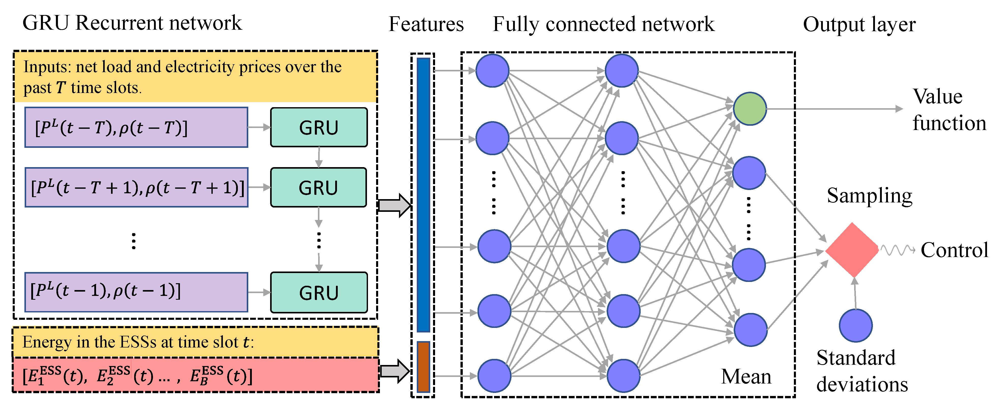
Figure 1. The architecture of the designed policy and value network. The overall network includes three parts: (1) the GRU network, which takes as inputs the net load and electricity prices of the past T time slots and outputs features about their future trends; (2) the feed-forward network, which concatenates the features extracted by GRU and the energy of ESSs at time slot t; and (3) the output layer outputs the approximated value function and the control policy.
Energies 14 02120 g001
Figure 2. The architecture of CIGRE low-voltage Microgrid.
Energies 14 02120 g002
Figure 3. Comparison of MPC, ADP, GA, and the proposed approach on 113 testing days. (a) Cumulative operating costs; (b) Optimization Error.
Energies 14 02120 g003
Figure 4. Training performance of DQN and the proposed approach (PPO). (a) Mean and 95% confidence interval of episode rewards over five random runs; (b) Mean and 95% confidence interval of imbalance power over five random runs.
Energies 14 02120 g004
Figure 5. Testing performance of DQN and the proposed approach (PPO). (a) Cumulative operating costs on 113 testing days; (b) Total imbalance power on each testing day.
Energies 14 02120 g005
Figure 6. Training performance of DDPG, TRPO, and the proposed approach (PPO). (a) Mean and 95% confidence interval of episode reward over five random runs; (b) Mean and 95% confidence interval of imbalance power over five random runs.
Energies 14 02120 g006
Figure 7. Testing performance of DDPG, TRPO, and the proposed approach (PPO). (a) Cumulative operating costs on 113 testing days; (b) Total imbalance power on each testing day.
Energies 14 02120 g007
Figure 8. Online scheduling decisions made by the proposed algorithm on seven consecutive test days. (a) Hourly electricity prices and net load; (b) Charging-discharging power and SOC pattern of the battery; (c) Power output of the DGs and the power exchange between the microgrid and utility grid; (d) Power curtailment of controllable loads.
Energies 14 02120 g008aEnergies 14 02120 g008b
Table 1. Parameters of the controllable devices in the microgrid.
DG1 P ̲ 1 DG P ¯ 1 DG a 1 b 1 c 1
0 kW30 kW 0.0001 $/kW 2 h 0.0716 $/kWh 0.04615 $/h
DG2 P ̲ 2 DG P ¯ 2 DG a 2 b 2 c 2
0 kW40 kW 0.0001 $/kW 2 h 0.0504 $/kWh 0.11011 $/h
ESS E ̲ 1 ESS E ¯ 1 ESS P ¯ 1 ESS η 1 c h η 1 d c h
50 kWh500 kWh100 kW 0.98 0.98
CL1 P ̲ 1 CL P ¯ 1 CL β 1
0 kW20 kW 0.003 $/kW 2 h
CL2 P ̲ 2 CL P ¯ 2 CL β 2
0 kW15 kW 0.004 $/kW 2 h
Table 2. Parameters of the PPO-based method for the Online Energy Scheduling Problem.
HyperparameterValue
# of steps in one episode (T)24
# of episodes in each iteration (N)100
# of iterates (I)1000
# of epochs (K)10
Discount factor ( γ ) 0.995
Adam stepsize 0.001
Minibatch size (M)64
GAE parameter ( λ )0.95
Penalty coefficient ( ω )5
Vf coefficient ( κ 1 )0.5
Entropy coefficient ( κ 2 )0.01
Table 3. Computation time at each time step during the online execution.
MethodADPGAMPCPPO
Time57.71 ± 13.85 ms9317.29 ± 1912.83 ms228.68 ± 116.20 ms0.50 ± 0.11 ms
Publisher’s Note: MDPI stays neutral with regard to jurisdictional claims in published maps and institutional affiliations.