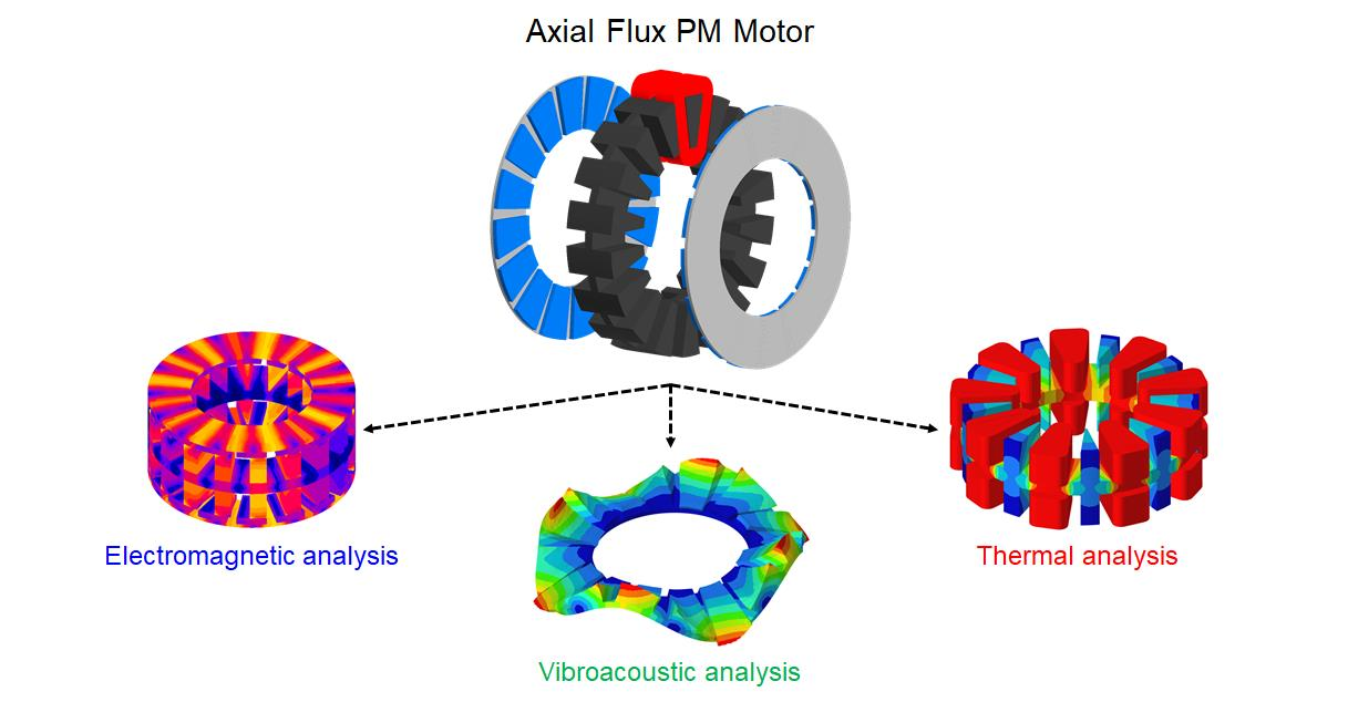
The components of the AFPM motor vary with its radius and this makes the analysis more complicated: thus, 3D FE analyses have been conducted through the Altair tools. Particularly, a 3D multiphysics analysis allowed the evaluation of not only the motor performance, but also the thermal behavior and the electromagnetic forces acting on the surfaces of the stator teeth and of the permanent magnets.
4.1. Electromagnetic Analyses
3D electromagnetic analyses have been carried out in order to evaluate the performance of the AFPM motor and its magnetic field distribution: static analyses have been performed to shorten the simulation time. A temperature of 100 °C has been imposed for both the stator windings and the permanent magnets.
Table 3 lists the motor performance at base speed and at maximum speed, and it fully satisfies the initial requirements with an efficiency higher than 80%.
The Back ElectroMotive Force (BEMF) at no-load is shown in
Figure 6 and it exhibits a sinusoidal behavior, while
Figure 7 presents the motor torque profile: the ripple, calculated as the ratio of the difference between the maximum and the minimum torque values to the average one, is very low and this is mainly due to the use of concentrated windings and to the right choice of the combination N. poles-N. slots.
The 3D on-load analysis allowed the evaluation of the flux density distributions (
Figure 8) in the AFPM motor; the maximum values in the stator teeth and in the stator yoke are about 2.4 T and this value is reasonable thanks to the use of the Fe-Co electrical steel, which has a high saturation value.
The Torque-Speed curve is reported in
Figure 9 and it points out a constant torque of about 78 Nm up to 840 rpm and a torque of about 68 Nm at maximum speed (1200 rpm).
Moreover,
Table 4 shows the motor losses during its on-load operation at different working points: in this way, it is possible to evaluate the motor performance and efficiency for many speed points, which is important for traction applications. As it can be seen, the Joule losses remain the same since the current value is constant and the current control angle changes, hence changing the d-axis and q-axis current components; all the other losses increase together with the operating speed of the electric motor (i.e., the iron losses depend on the frequency value). Although, it can be noticed that the efficiency does not decrease in the flux-weakening region, making the motor meet the efficiency requirements for this kind of application.
4.2. Noise and Vibration Analyses
The NVH (Noise, Vibration and Harshness) analysis in the automotive field is necessary in order to evaluate the vehicle’s comfort and to make it comply with the environmental requirements, since the motor can be a great source of noise and vibrations if not properly designed and controlled [
16]. The reason why the electric motor can produce noise has to be found in the magnetic forces acting between the stator teeth and the rotor permanent magnets [
17,
18].
Three main categories of vibrations and noise produced by an electrical machine can be defined: the electromagnetic vibrations and noise (due to higher harmonics of time and space, phase unbalance, magnetic saturation, slot openings, magnetostriction, etc.), the mechanical ones (due to bearings, rotor unbalance, shaft misalignment, etc.) and the aerodynamic ones (due to the air flow produced by the cooling fan, etc.).
In particular, in this case study, the modal analysis of the electrical machine’s mechanical system (complete with housing and shaft) and the frequency response on a modal basis have been carried out. The first analysis has provided the natural frequencies and the mode shapes of the mechanical structure, in order to check if any frequency of the Maxwell forces between the stator and the rotor matched them, either spatially and temporally: this would cause the so-called resonance phenomenon, a dynamic effect that amplifies noise and vibrations, making them dangerous for the motor’s integrity.
In order to carry out a realistic vibroacoustic analysis and to obtain accurate results, the machine’s geometry used for the electromagnetic analyses must be mirrored first and then completed with the addition of the shaft and of the housing. The mechanical system of the axial flux permanent magnet machine is shown in
Figure 10. It is possible to see the second-order tetrahedral mesh that has been created after many attempts at finding the proper element size for each component; in fact, the mesh elements have to be small enough to obtain accurate results but not too much to excessively increase the computational time.
The modal and frequency response analyses have been realized with another Finite Element Analysis (FEA) tool of the Altair Suite: HyperWorks. After defining the mechanical properties of each component’s material (
Table 5), the entities that define the bearings, which connect the shaft to the housing, and the flanges, which connect the rotor discs to the shaft, have been created. Moreover, the contacts between the stator teeth and the windings and between the stator teeth and the housing have been defined and the clamped-condition for one side of the housing has been set.
Finally, the electromagnetic torque and the normal component of the global magnetic forces due to the stator-PMs interaction (while in
Figure 11 the nodal magnetic forces are shown) have been exported from Altair Flux and imported into HyperWorks as loads of the studied mechanical system: specifically, the global Maxwell forces have been applied to both the surface sets of the rotor permanent magnets and of the stator teeth facing each other, while the electromagnetic torque has been applied as a distributed load to all the surfaces of the stator teeth facing the air gap. In
Figure 12, the Fast Fourier Transform (FFT) of the axial magnetic forces on one permanent magnet’s face is shown.
The frequency range set for the frequency response analysis goes from to and the chosen outputs are: the displacement, the velocity and the acceleration of each system’s point. Therefore, the results have been analyzed only for several characteristic points, but just the main ones are addressed in this paper: one point at the center of one stator tooth facing the air gap and another one at the radially outer point on the upper rotor’s disc. It can be stated that some harmonic components of the magnetic forces match the structure’s natural frequencies, leading to resonance phenomena in correspondence of two resonance frequencies: and .
Figure 13 shows the stator deformed geometry’s velocities at
, which is the frequency at which there are both the peak value of the teeth’s displacement and their maximum displacements’ velocity; in fact, as it can be seen in
Figure 14, the maximum displacement’s velocity is equal to
at the resonance frequency of
, while the peak value of the teeth’s displacement is equal to
at the same frequency.
Figure 15 shows the rotor deformed geometry’s displacements of the AFPM machine at the resonance frequency of
, while
Figure 16 displays the rotor discs’ displacements, whose peak values are equal to
for the z-axis direction at both the mechanical system’s natural frequencies of
and
; the values of the displacements are acceptable and do not interfere with the operating conditions of the machine, since it is clear that the rotor discs, and hence the permanent magnets (with a maximum displacement’s value of
), do not touch the inner stator. Regarding the deformed geometry’s velocities of the rotor’s disc, the maximum value at
is equal to
.
With regard to the noise produced by an electrical machine, it can be stated that more vibrations produce more sound. There are different parameters that can affect a machine’s sound radiation: its dimensions, its material properties, the excitations and the conditions of the surroundings. There are two types of noise: the structure-borne one, which is caused by the vibrations of solid objects, and the air-borne noise, caused by the movement of large air volumes or by the use of high-pressure.
In order to quantify the variations in the sound pressure of an ambient, the logarithmic expression of the Sound Pressure Level (SPL) can be used: the SPL characterizes the loudness of the sound level of an ambient; it depends on the distance from the noise source and it is expressed in decibels (dB):
where
is the sound pressure and
is the rms value of the reference sound pressure.
In order to evaluate the noise produced by the vibrations of the analyzed AFPM motor, a sphere of 1 meter radius has been created in HyperWorks: each node of the sphere’s elements corresponds to a microphone that records the sound level in the acoustic field around the machine, as visible in
Figure 17. To obtain the sound radiated by the noise source, the SPL has been set as another output of the frequency response analysis and the housing’s external faces have been chosen to be the radiating panels, since they are responsible for the propagation of the machine’s sound towards the surroundings.
The speed of sound has been set at , the acoustic medium’s density has been set at and the sound pressure reference value has been set at .
Figure 18 shows the contour plot of the sound pressure levels around the machine at the resonance frequency of
, while
Figure 19 displays the SPL detected by the sphere’s microphones in the red zone: the maximum sound pressure level obtained by those microphones and, hence, radiated by the AFPM machine during its nominal operating conditions reaches the value of
, which is acceptable for this type of application.
4.3. Thermal Analysis
Thermal analyses are of great relevance, especially concerning PM machines because of the permanent magnet sensitivity to high operating temperatures, which could lead to the PM demagnetization. In order to avoid that and to ensure the AFPM motor reliability, a thermal analysis has been carried out with the Altair Finite Element Method (FEM) software used for Computational Fluid Dynamics (CFD) simulations: in this workspace, the conductive heat transfers have been modeled and the convective ones have been imposed; however, the fluid dynamics has been neglected in this context. Considering the chosen cooling system (forced-air) and the base speed working point, it has been possible to establish whether the insulating materials, the bearings and the permanent magnets could be damaged by high temperatures, which could have also caused higher losses and, therefore, a lower efficiency of the electric machine.
The machine losses have been considered as heat sources: the main ones are due to the Joule losses, to the stator and rotor iron losses and to the PM losses, while the other contributions are lower and, therefore, they have not been considered in this 3D FE simulation [
19]. The material thermal properties have been assigned to each machine’s component, as it can be seen in
Table 6.
After that each material has been assigned to the correspondent components, it has been possible to define the internal heat sources starting from the machine losses mentioned above: their values are shown in
Table 7.
Considering a forced-air cooling system, which has been chosen to provide a better cooling of the machine than the one provided by a natural-air cooling system, the convective heat transfer coefficients have been empirically estimated to determine the boundary conditions for the CFD simulation. Some assumptions must be made: one side of the AFPM motor housing is clamped to the chassis of the vehicle; the rotor rings are keyed to the inner side of the wheel’s rim (with a 24 cm radius); the ambient temperature is equal to 20 °C. Assuming that the motor base speed corresponds to 21 m/s of the electric vehicle’s wheels and that some housing’s areas are directly hit by the air while others are less or by no means lapped by it, the average convective heat transfer coefficient used for the external housing’s surfaces (except for the one clamped to the chassis) can be seen in
Table 8. The other coefficients have been estimated considering that inside the machine’s housing there is an improvement in the quality of the thermal exchange, which is mainly due to the turbulent motion of the two rotor discs and that depends almost linearly on the rotating speed and on the average diameter of the discs. Considering the faces of the permanent magnets and of the stator teeth that face the air gap, they do not benefit from a great air circulation because of the little space defined by the motor air gap itself; therefore, their convective heat transfer coefficient is quite low.
Once the mesh has been created and considering the conductive and convective heat transfers between the machine’s components, the thermal analysis has been carried out and the temperature distributions shown in the following figures have been obtained.
In
Figure 20, it is possible to notice that the maximum temperature reached by the housing is equal to 77 °C, while the one reached by the shaft is about 30 °C.
Figure 21 shows the temperature distribution within the active materials of the AFPM motor, whose average temperature is about 70 °C. In
Figure 22, the PM and the rotor disc temperatures are displayed: the maximum temperature reached by the PMs is equal to 42 °C, whose value prevents the PMs from being demagnetized. The stator core is characterized by an average temperature of 87 °C, while the hottest spot has been detected in the windings that reach a maximum temperature of 105 °C, as it can be seen in
Figure 23. Therefore, the temperature considered for the windings in the electromagnetic analyses matches the one resulting from the thermal simulation; besides, the insulation class required for this electric motor is the F-class, whose maximum operating temperature corresponds to 155 °C; this choice allows the motor to work in overload conditions for short periods of time without damaging the materials.


 ,
, 


