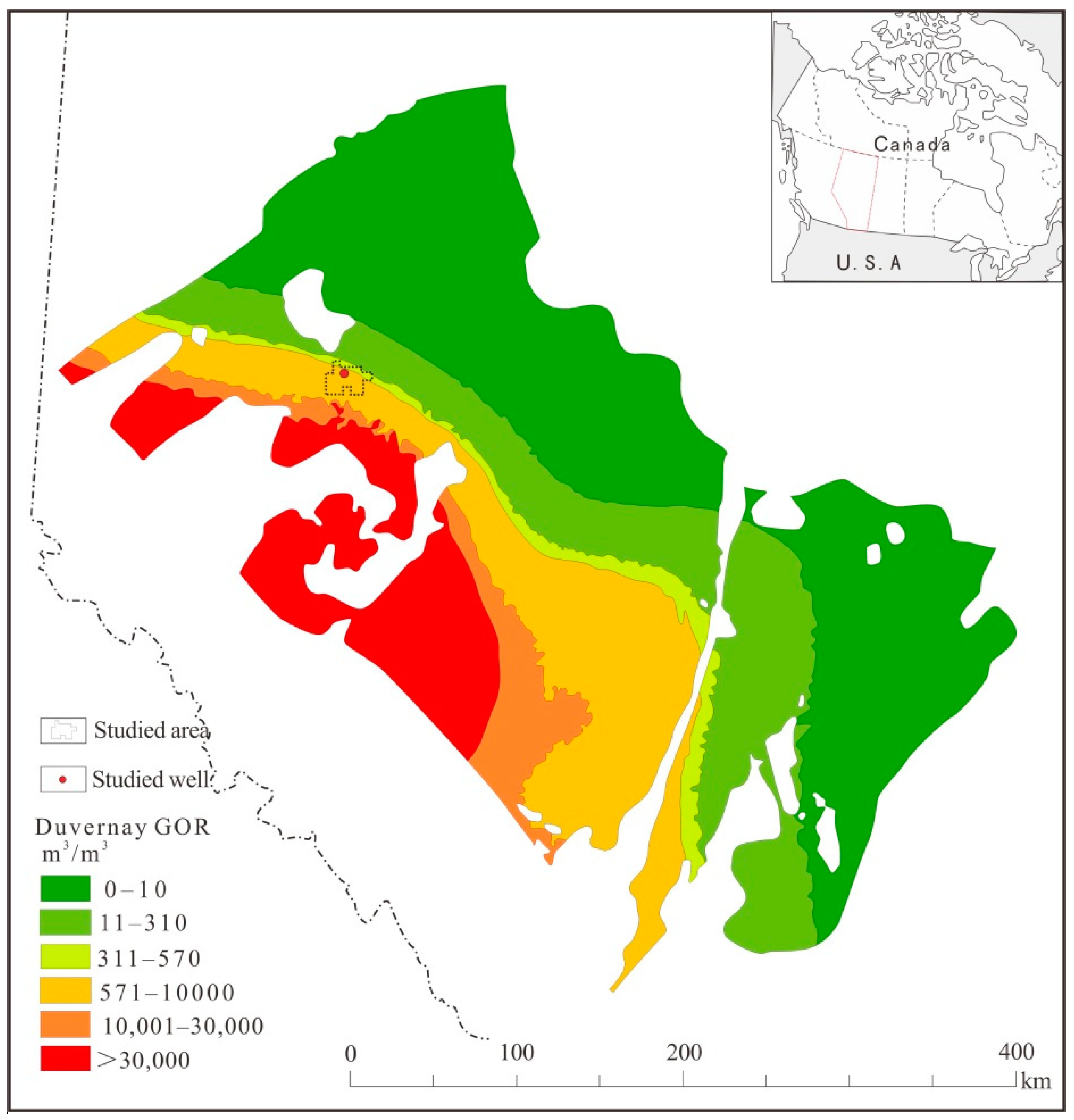
Figure 1.
Gas-to-oil ratio (GOR) in the Duvernay shale and the location of the subject well (after Lyster et al. 2017) [
23].
Figure 1.
Gas-to-oil ratio (GOR) in the Duvernay shale and the location of the subject well (after Lyster et al. 2017) [
23].
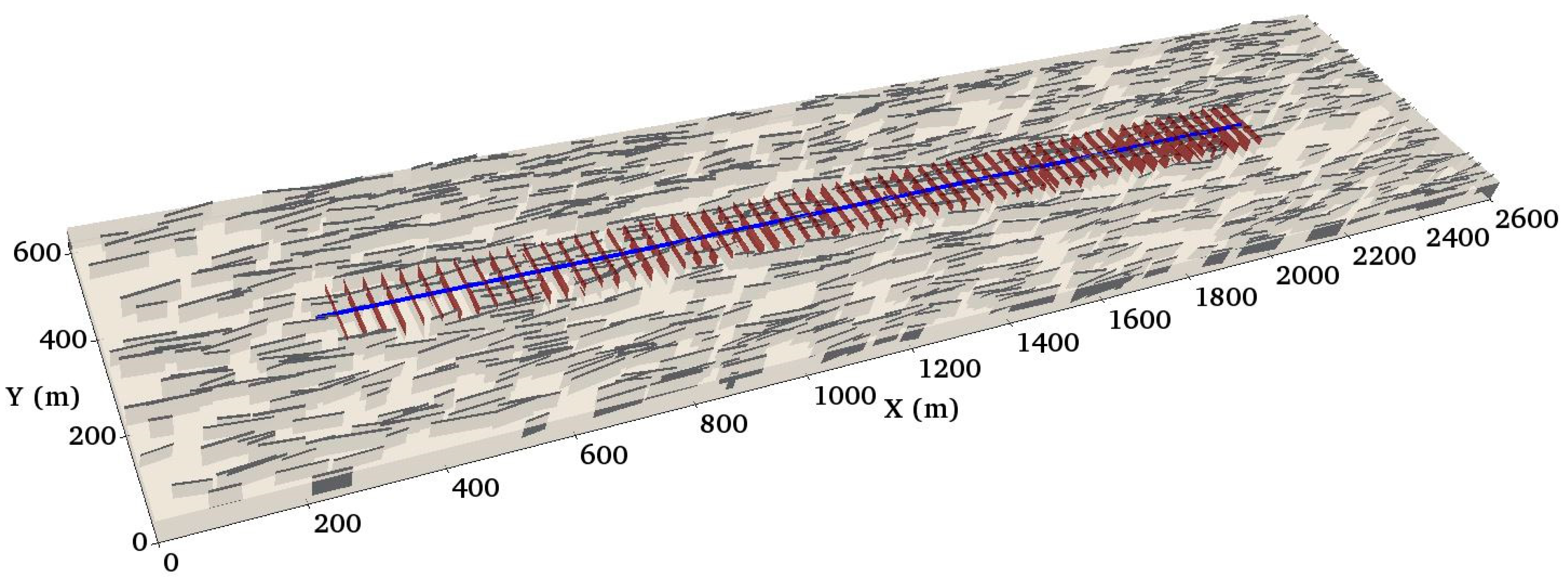
Figure 2.
Numerical model with hydraulic fractures (in red) and natural fractures (in grey).
Figure 2.
Numerical model with hydraulic fractures (in red) and natural fractures (in grey).
Figure 3.
Comparison of well performance between raw data and model results: (a) Bottomhole Pressure; (b) Oil Rate; (c) Gas Rate.
Figure 3.
Comparison of well performance between raw data and model results: (a) Bottomhole Pressure; (b) Oil Rate; (c) Gas Rate.
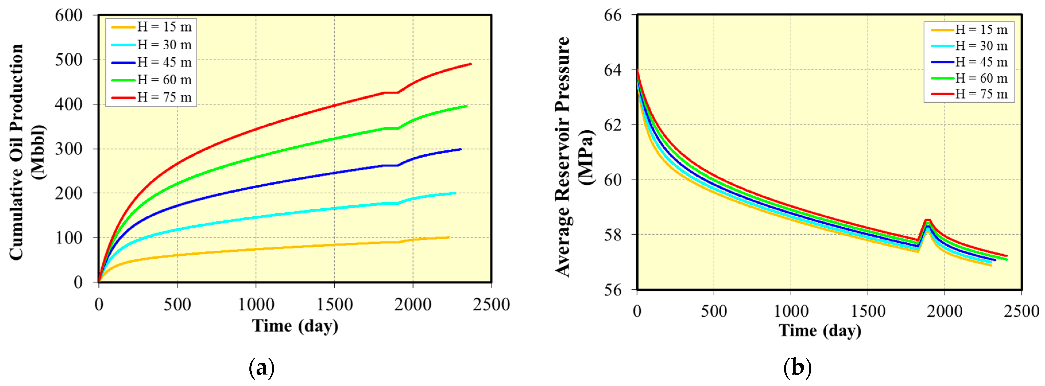
Figure 4.
Effect of different reservoir thickness with one huff-n-puff cycle on oil production and reservoir pressure: (a) Cumulative oil production for different reservoir thickness; (b) Average reservoir pressure for different reservoir thickness.
Figure 4.
Effect of different reservoir thickness with one huff-n-puff cycle on oil production and reservoir pressure: (a) Cumulative oil production for different reservoir thickness; (b) Average reservoir pressure for different reservoir thickness.
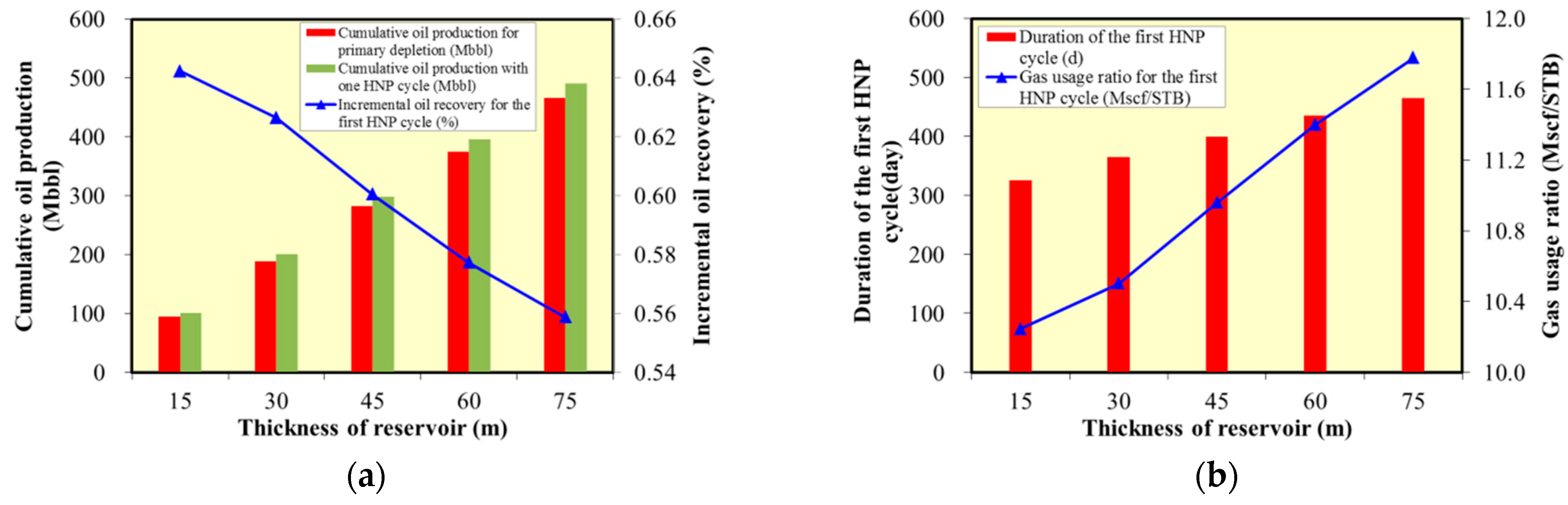
Figure 5.
Correlation between reservoir thickness and huff-n-puff results: (a) Cumulative oil production and incremental oil recovery for different reservoir thickness; (b) Duration of the first huff-n-puff cycle and gas usage ratio for different reservoir thickness.
Figure 5.
Correlation between reservoir thickness and huff-n-puff results: (a) Cumulative oil production and incremental oil recovery for different reservoir thickness; (b) Duration of the first huff-n-puff cycle and gas usage ratio for different reservoir thickness.
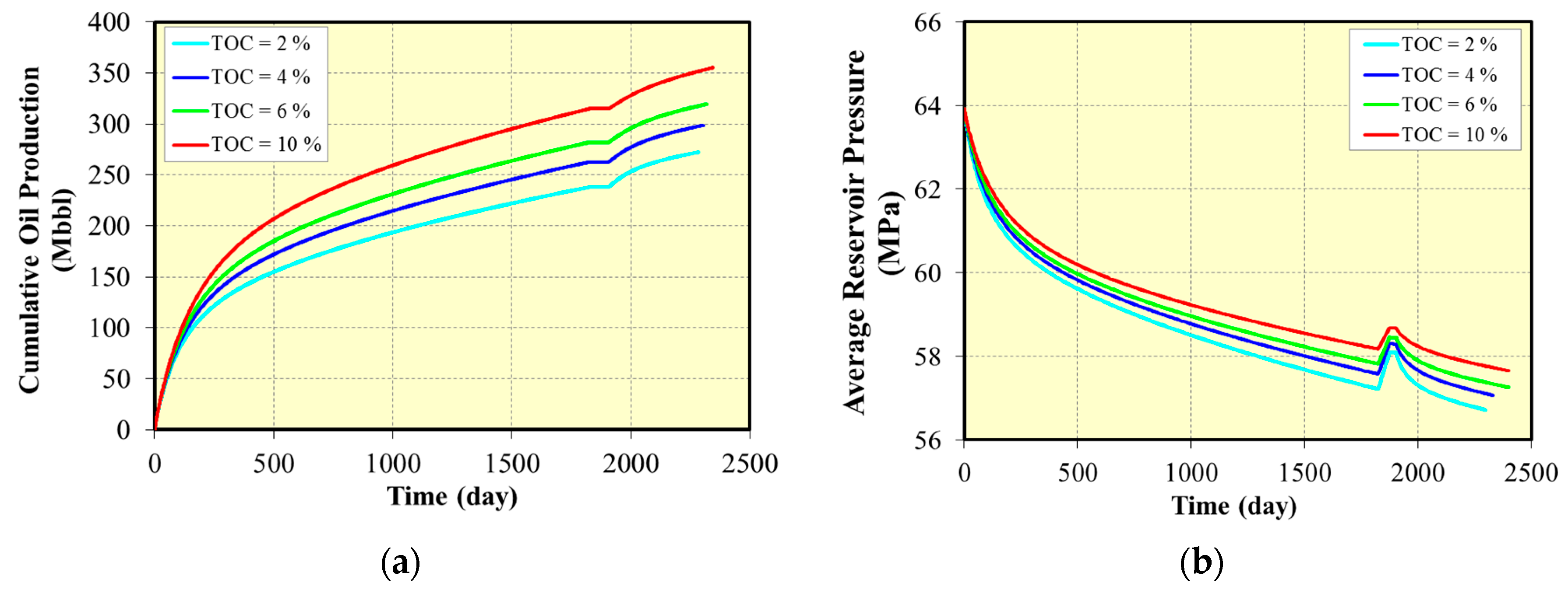
Figure 6.
Effect of different TOC with one huff-n-puff cycle on oil production and reservoir pressure: (a) Cumulative oil production for different TOC; (b) Average reservoir pressure for different TOC.
Figure 6.
Effect of different TOC with one huff-n-puff cycle on oil production and reservoir pressure: (a) Cumulative oil production for different TOC; (b) Average reservoir pressure for different TOC.
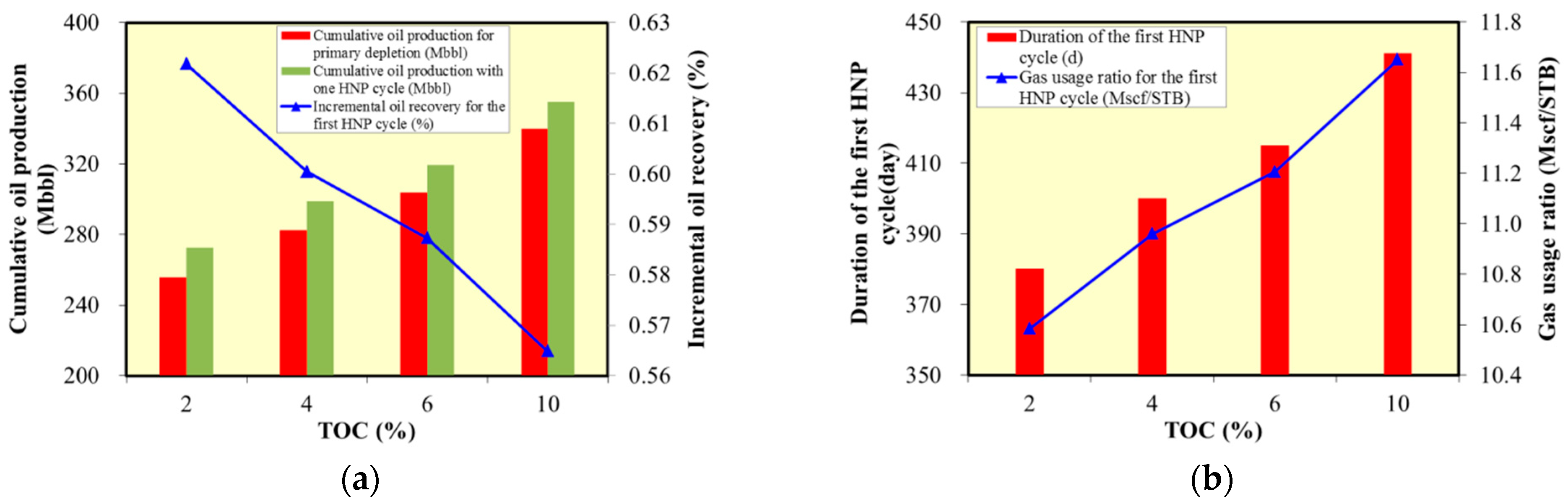
Figure 7.
Correlation between TOC and huff-n-puff results: (a) Cumulative oil production and incremental oil recovery for different TOC; (b) Duration of the first huff-n-puff cycle and gas usage ratio for different TOC.
Figure 7.
Correlation between TOC and huff-n-puff results: (a) Cumulative oil production and incremental oil recovery for different TOC; (b) Duration of the first huff-n-puff cycle and gas usage ratio for different TOC.
Figure 8.
Effect of different pore radius of shale matrix with one huff-n-puff cycle on oil production and reservoir pressure: (a) Cumulative oil production for different pore radius of shale matrix; (b) Average reservoir pressure for different pore radius of shale matrix.
Figure 8.
Effect of different pore radius of shale matrix with one huff-n-puff cycle on oil production and reservoir pressure: (a) Cumulative oil production for different pore radius of shale matrix; (b) Average reservoir pressure for different pore radius of shale matrix.
Figure 9.
Correlation between pore radius of shale matrix and huff-n-puff results: (a) Cumulative oil production and incremental oil recovery for different pore radius of shale matrix; (b) Duration of the first huff-n-puff cycle and gas usage ratio for different pore radius of shale matrix.
Figure 9.
Correlation between pore radius of shale matrix and huff-n-puff results: (a) Cumulative oil production and incremental oil recovery for different pore radius of shale matrix; (b) Duration of the first huff-n-puff cycle and gas usage ratio for different pore radius of shale matrix.
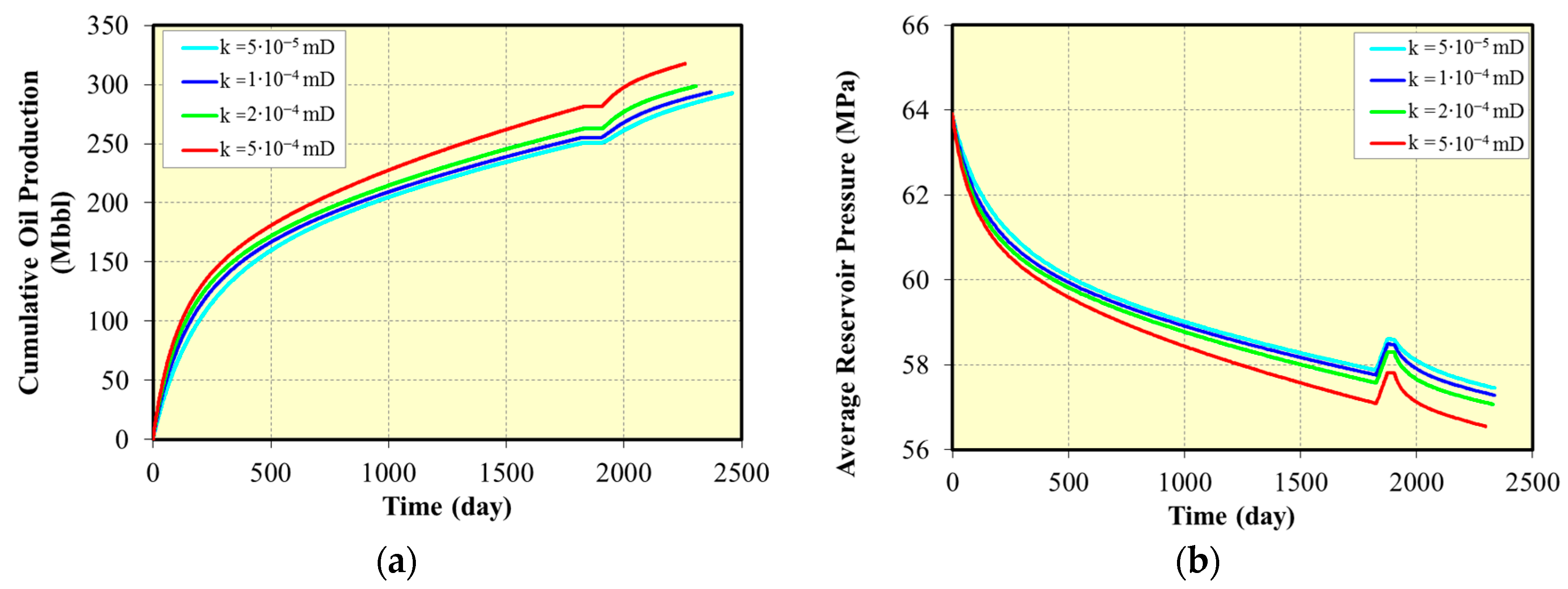
Figure 10.
Effect of different matrix permeability with one huff-n-puff cycle on oil production and reservoir pressure: (a) Cumulative oil production for different matrix permeability; (b) Average reservoir pressure for different matrix permeability.
Figure 10.
Effect of different matrix permeability with one huff-n-puff cycle on oil production and reservoir pressure: (a) Cumulative oil production for different matrix permeability; (b) Average reservoir pressure for different matrix permeability.
Figure 11.
Correlation between matrix permeability and huff-n-puff results: (a) Cumulative oil production and incremental oil recovery for different matrix permeability; (b) Duration of the first huff-n-puff cycle and gas usage ratio for different matrix permeability.
Figure 11.
Correlation between matrix permeability and huff-n-puff results: (a) Cumulative oil production and incremental oil recovery for different matrix permeability; (b) Duration of the first huff-n-puff cycle and gas usage ratio for different matrix permeability.
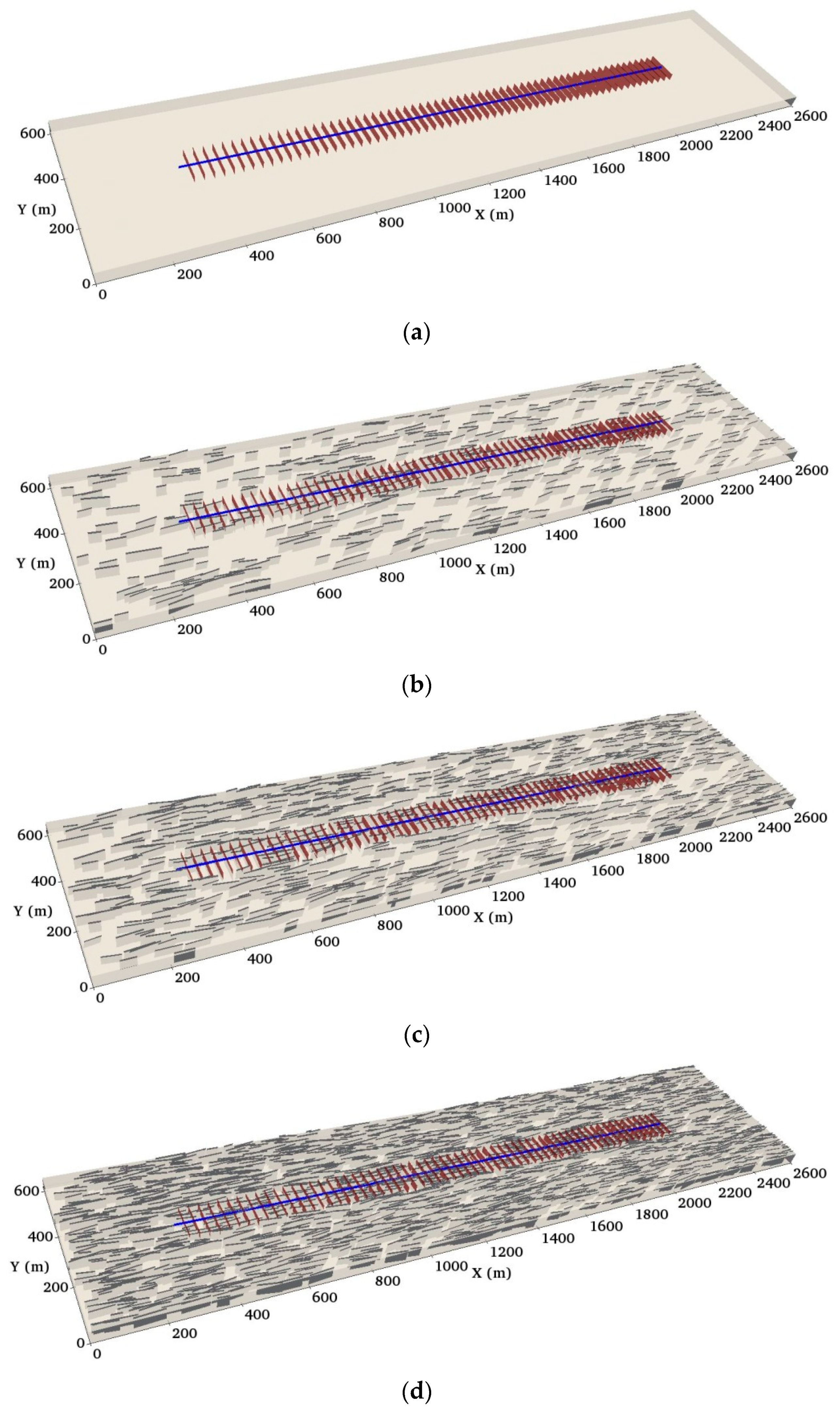
Figure 12.
Numerical model with complex fractures: (a) without natural fractures; (b) 0.05 natural fracture/m; (c) 0.1 natural fracture/m; (d) 0.2 natural fracture/m; (e) 0.5 natural fracture/m. Blue line indicates the wellbore. Red and grey pieces represent hydraulic fractures and natural fractures respectively.
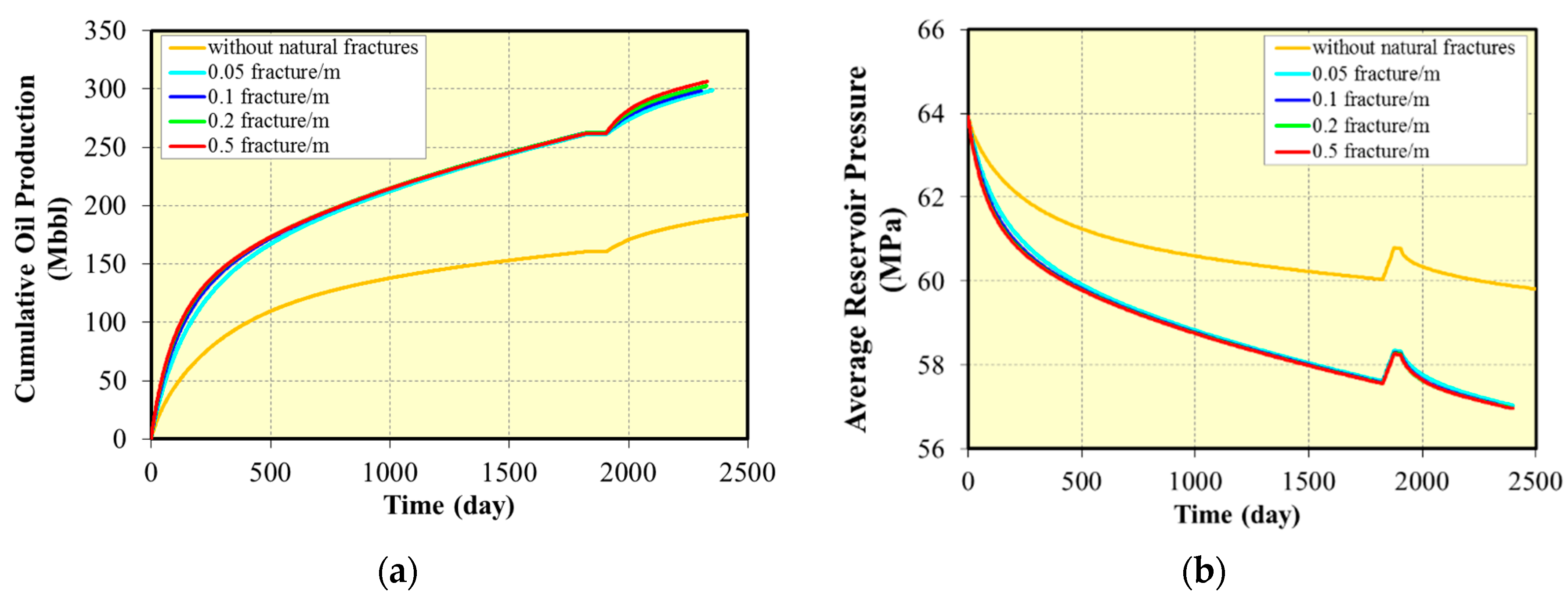
Figure 13.
Effect of different natural fracture densities with one huff-n-puff cycle on oil production and reservoir pressure: (a) Cumulative oil production for different natural fracture densities; (b) Average reservoir pressure for different natural fracture densities.
Figure 13.
Effect of different natural fracture densities with one huff-n-puff cycle on oil production and reservoir pressure: (a) Cumulative oil production for different natural fracture densities; (b) Average reservoir pressure for different natural fracture densities.
Figure 14.
Correlation between natural fracture density and huff-n-puff results: (a) Cumulative oil production and incremental oil recovery for different natural fracture densities; (b) Duration of the first huff-n-puff cycle and gas usage ratio for different natural fracture densities.
Figure 14.
Correlation between natural fracture density and huff-n-puff results: (a) Cumulative oil production and incremental oil recovery for different natural fracture densities; (b) Duration of the first huff-n-puff cycle and gas usage ratio for different natural fracture densities.
Figure 15.
Effect of different natural fracture permeability with one huff-n-puff cycle on oil production and reservoir pressure: (a) Cumulative oil production for different natural fracture permeability; (b) Average reservoir pressure for different natural fracture permeability.
Figure 15.
Effect of different natural fracture permeability with one huff-n-puff cycle on oil production and reservoir pressure: (a) Cumulative oil production for different natural fracture permeability; (b) Average reservoir pressure for different natural fracture permeability.
Figure 16.
Correlation between natural fracture permeability and huff-n-puff results: (a) Cumulative oil production and incremental oil recovery for different natural fracture permeability; (b) Duration of the first huff-n-puff cycle and gas usage ratio for different natural fracture permeability.
Figure 16.
Correlation between natural fracture permeability and huff-n-puff results: (a) Cumulative oil production and incremental oil recovery for different natural fracture permeability; (b) Duration of the first huff-n-puff cycle and gas usage ratio for different natural fracture permeability.
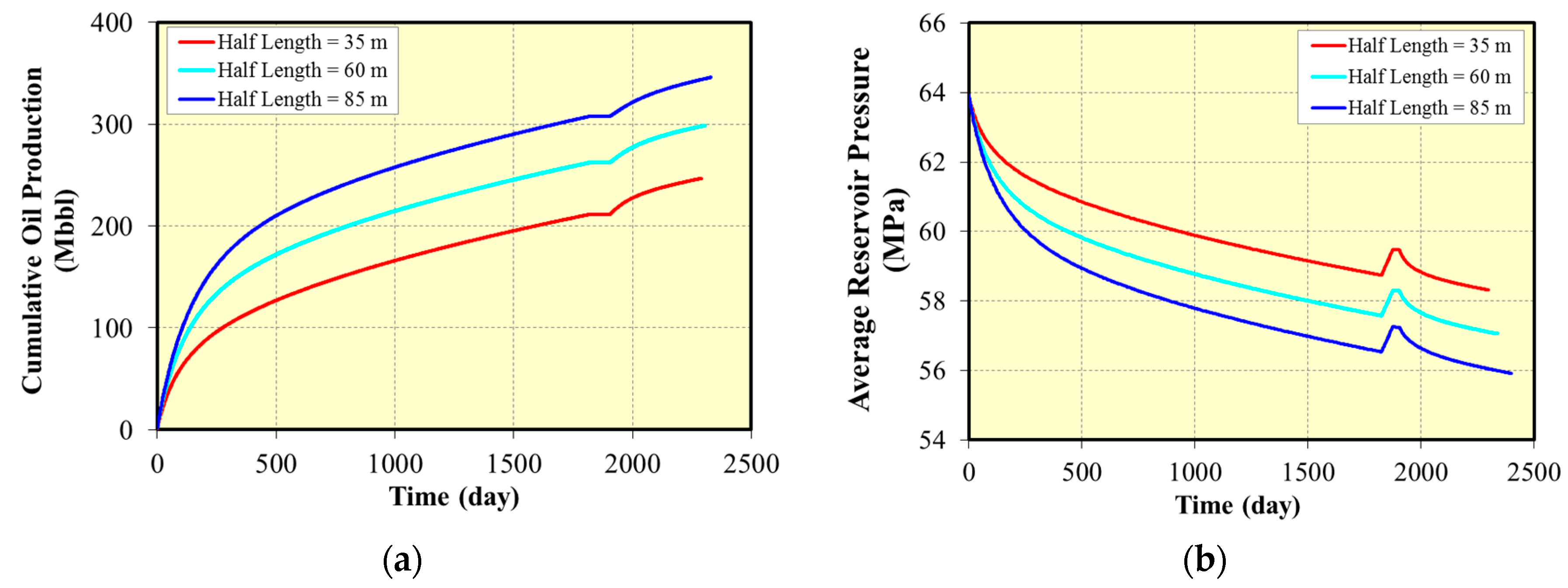
Figure 17.
Effect of different half-length of hydraulic fractures with one huff-n-puff cycle on oil production and reservoir pressure: (a) Cumulative oil production for different half-length of hydraulic fractures; (b) Average reservoir pressure for different half-length of hydraulic fractures.
Figure 17.
Effect of different half-length of hydraulic fractures with one huff-n-puff cycle on oil production and reservoir pressure: (a) Cumulative oil production for different half-length of hydraulic fractures; (b) Average reservoir pressure for different half-length of hydraulic fractures.
Figure 18.
The correlation between half-length of hydraulic fractures and huff-n-puff results: (a) Cumulative oil production and incremental oil recovery for different half-length of hydraulic fractures; (b) Duration of the first huff-n-puff cycle and gas usage ratio for different half-length of hydraulic fractures.
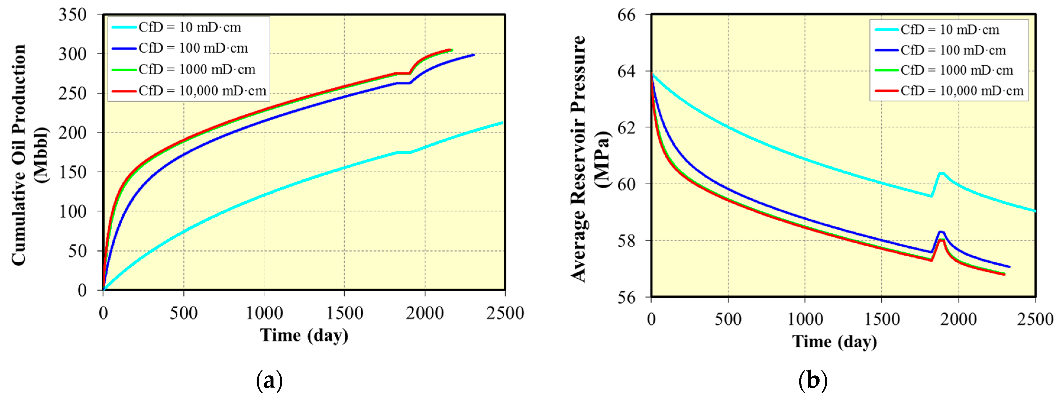
Figure 19.
Effect of different fracture conductivity with one huff-n-puff cycle on oil production and reservoir pressure: (a) Cumulative oil production for different fracture conductivity; (b) Average reservoir pressure for different fracture conductivity.
Figure 19.
Effect of different fracture conductivity with one huff-n-puff cycle on oil production and reservoir pressure: (a) Cumulative oil production for different fracture conductivity; (b) Average reservoir pressure for different fracture conductivity.
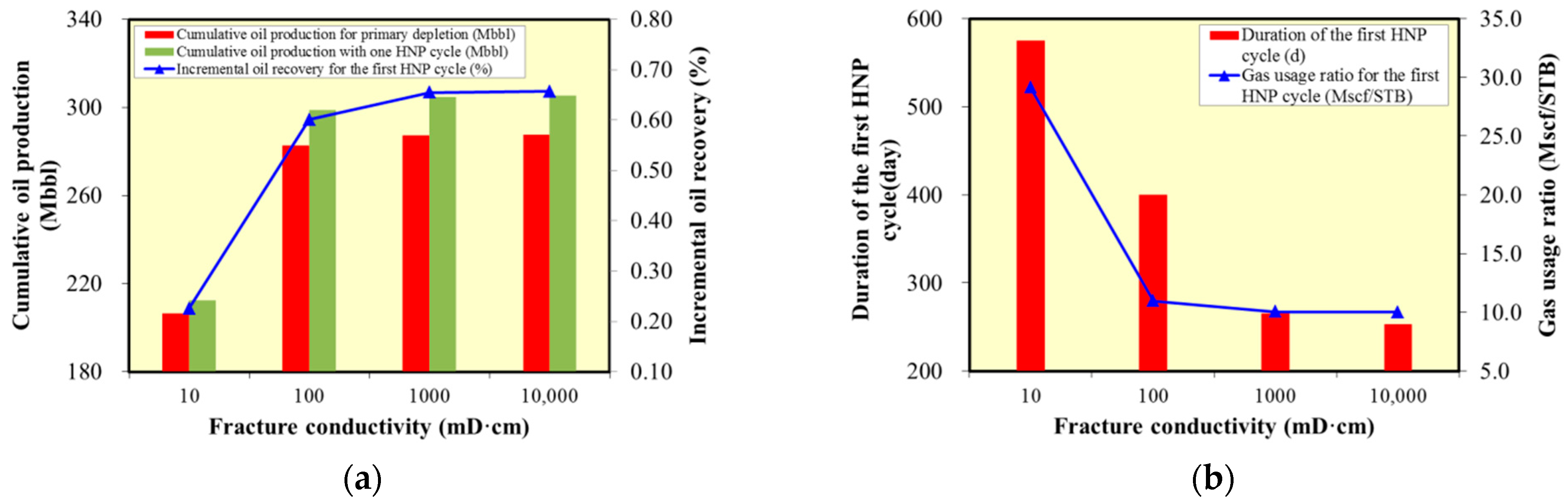
Figure 20.
Correlation between fracture conductivity and huff-n-puff results: (a) Cumulative oil production and incremental oil recovery for different fracture conductivity; (b) Duration of the first huff-n-puff cycle and gas usage ratio for different fracture conductivity.
Figure 20.
Correlation between fracture conductivity and huff-n-puff results: (a) Cumulative oil production and incremental oil recovery for different fracture conductivity; (b) Duration of the first huff-n-puff cycle and gas usage ratio for different fracture conductivity.
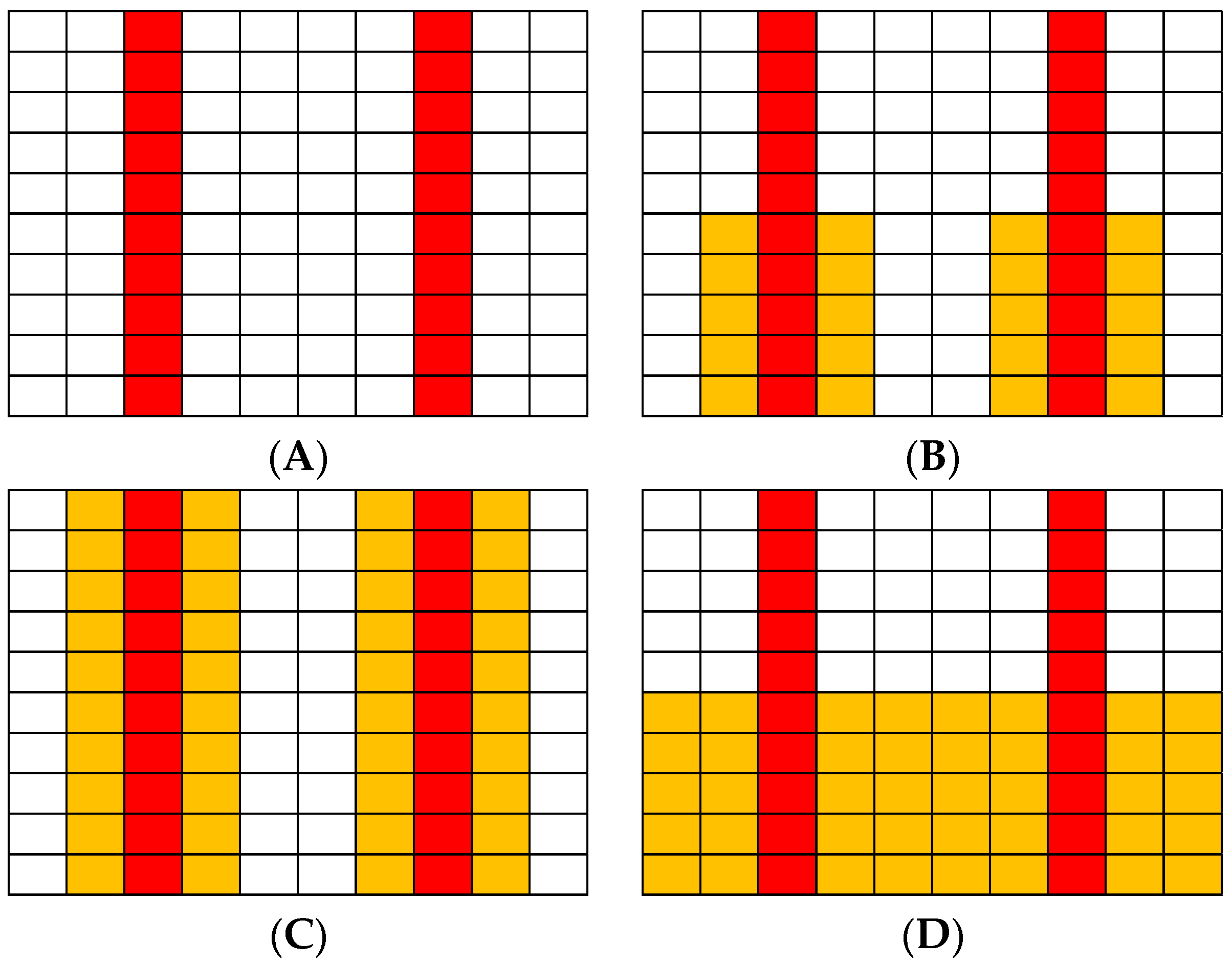
Figure 21.
Four types of SRV region: (A) No stimulation around main hydraulic fractures; (B) Stimulation within 10 m of the single wing; (C) Stimulation within 10 m of the bi-wing; (D) Stimulation within 20 m of the single wing. The red grid indicates hydraulic fractures. The orange grid represents the SRV region. The white grid denotes matrix.
Figure 22.
Effect of different types of SRV region with one huff-n-puff cycle on oil production and reservoir pressure: (a) Cumulative oil production for different types of SRV region; (b) Average reservoir pressure for different types of SRV region.
Figure 22.
Effect of different types of SRV region with one huff-n-puff cycle on oil production and reservoir pressure: (a) Cumulative oil production for different types of SRV region; (b) Average reservoir pressure for different types of SRV region.
Figure 23.
The correlation between types of SRV region and huff-n-puff results: (a) Cumulative oil production and incremental oil recovery for different types of SRV region; (b) Duration of the first huff-n-puff cycle and gas usage ratio for different types of SRV region.
Figure 23.
The correlation between types of SRV region and huff-n-puff results: (a) Cumulative oil production and incremental oil recovery for different types of SRV region; (b) Duration of the first huff-n-puff cycle and gas usage ratio for different types of SRV region.
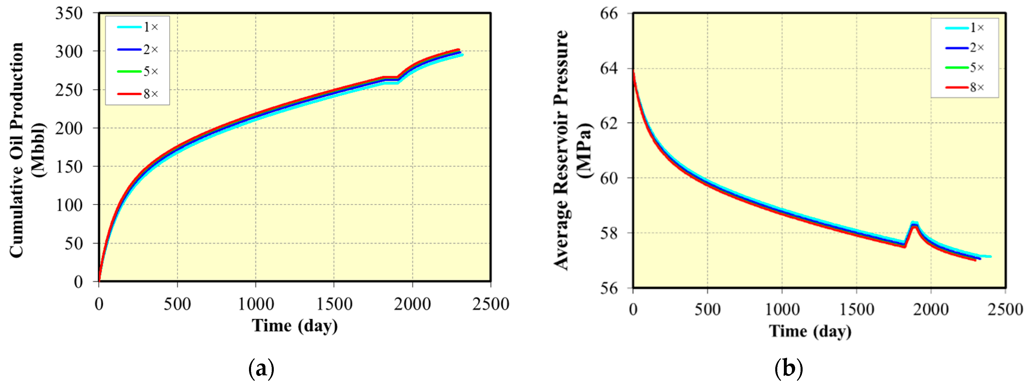
Figure 24.
Effect of different permeability magnifications in the SRV region with one huff-n-puff cycle on oil production and reservoir pressure: (a) Cumulative oil production for different magnification of permeability in SRV region; (b) Average reservoir pressure for different permeability magnifications in the SRV region.
Figure 25.
Correlation between magnification of permeability in SRV region and huff-n-puff results: (a) Cumulative oil production and incremental oil recovery for different magnification of permeability in SRV region; (b) Duration of the first huff-n-puff cycle and gas usage ratio for different magnification of permeability in SRV region.
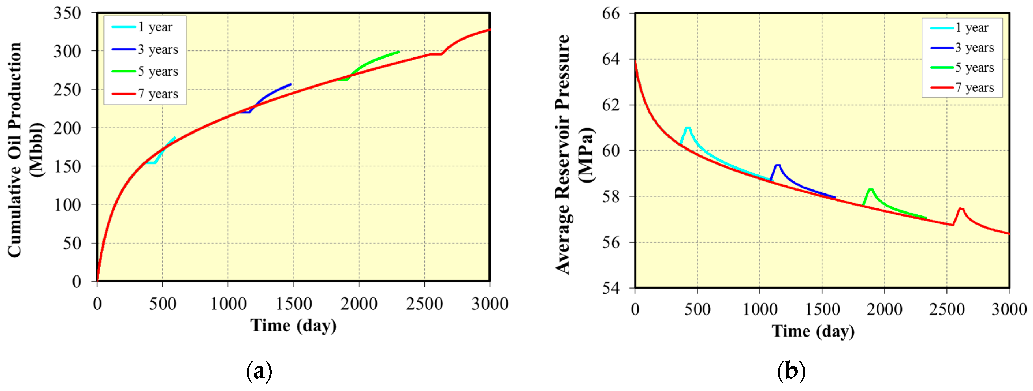
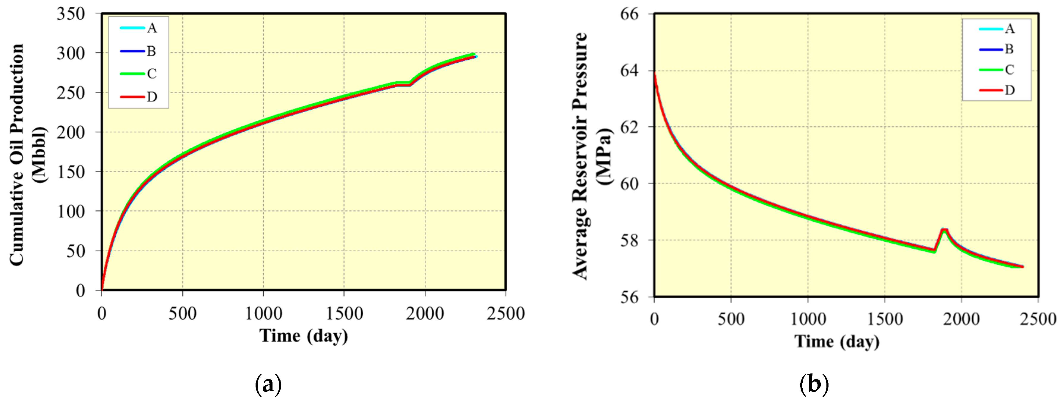
Figure 26.
Effect of different periods of primary depletion with one huff-n-puff cycle on oil production and reservoir pressure: (a) Cumulative oil production for different period of primary depletion; (b) Average reservoir pressure for different period of primary depletion.
Figure 26.
Effect of different periods of primary depletion with one huff-n-puff cycle on oil production and reservoir pressure: (a) Cumulative oil production for different period of primary depletion; (b) Average reservoir pressure for different period of primary depletion.
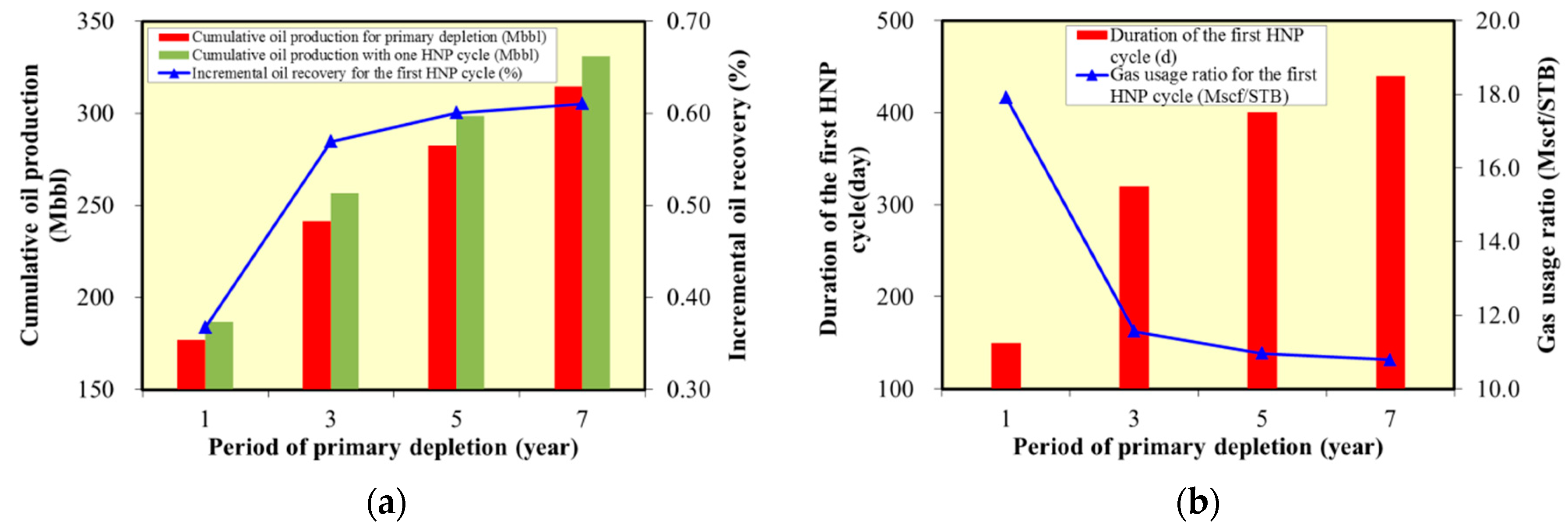
Figure 27.
Correlation between the periods of primary depletion and huff-n-puff results: (a) Cumulative oil production and incremental oil recovery for different periods of primary depletion; (b) Duration of the first huff-n-puff cycle and gas usage ratio for different periods of primary depletion.
Figure 27.
Correlation between the periods of primary depletion and huff-n-puff results: (a) Cumulative oil production and incremental oil recovery for different periods of primary depletion; (b) Duration of the first huff-n-puff cycle and gas usage ratio for different periods of primary depletion.
Figure 28.
Effect of different BHP of primary depletion with one huff-n-puff cycle on oil production and reservoir pressure: (a) Cumulative oil production for different BHP of primary depletion; (b) Average reservoir pressure for different BHP of primary depletion.
Figure 28.
Effect of different BHP of primary depletion with one huff-n-puff cycle on oil production and reservoir pressure: (a) Cumulative oil production for different BHP of primary depletion; (b) Average reservoir pressure for different BHP of primary depletion.
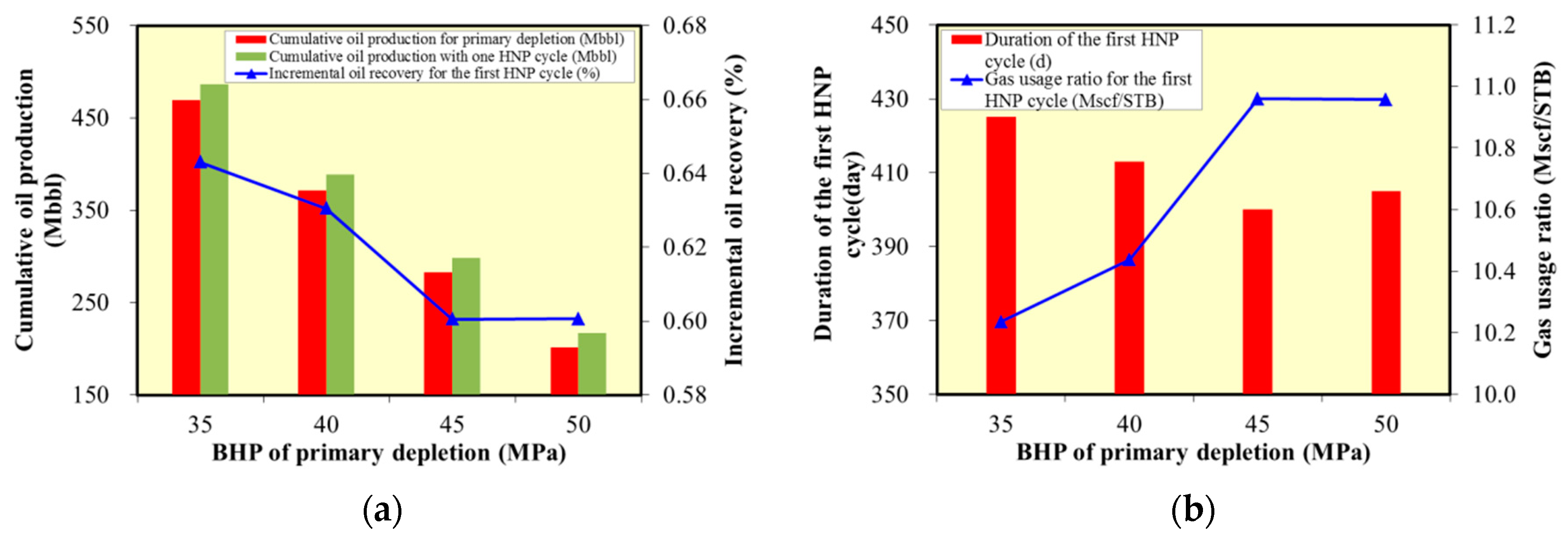
Figure 29.
The correlation between BHP of primary depletion and huff-n-puff results: (a) Cumulative oil production and incremental oil recovery for different BHP of primary depletion; (b) Duration of the first huff-n-puff cycle and gas usage ratio for different BHP of primary depletion.
Figure 29.
The correlation between BHP of primary depletion and huff-n-puff results: (a) Cumulative oil production and incremental oil recovery for different BHP of primary depletion; (b) Duration of the first huff-n-puff cycle and gas usage ratio for different BHP of primary depletion.
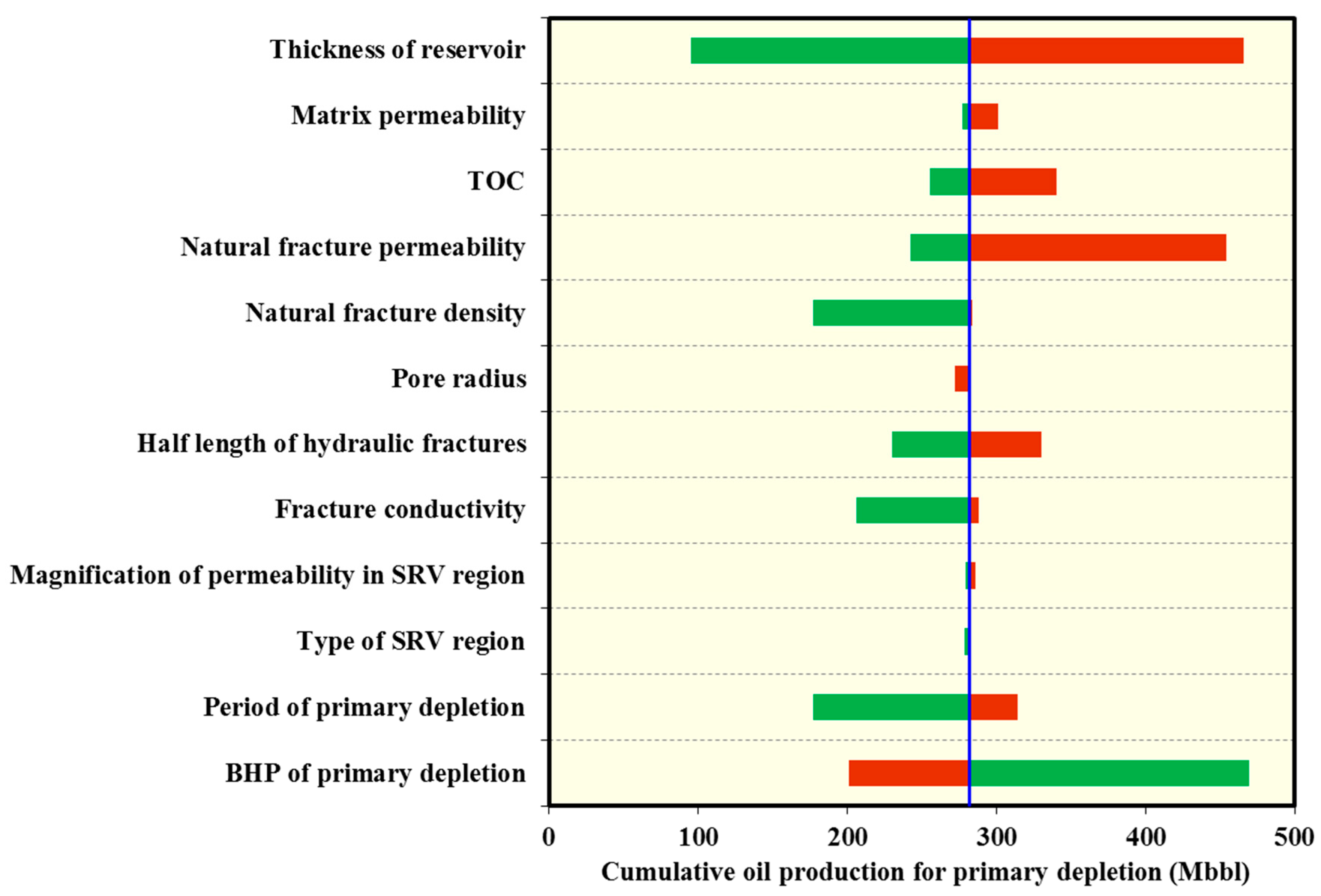
Figure 30.
Tornado chart indicating the most and least sensitive parameters for cumulative oil production for primary depletion. Each green bar corresponds to a sensitivity measure (compared to a base case) when a parameter is set to its lower bound. The red bars are for the upper bounds. The vertical blue line denotes the base case.
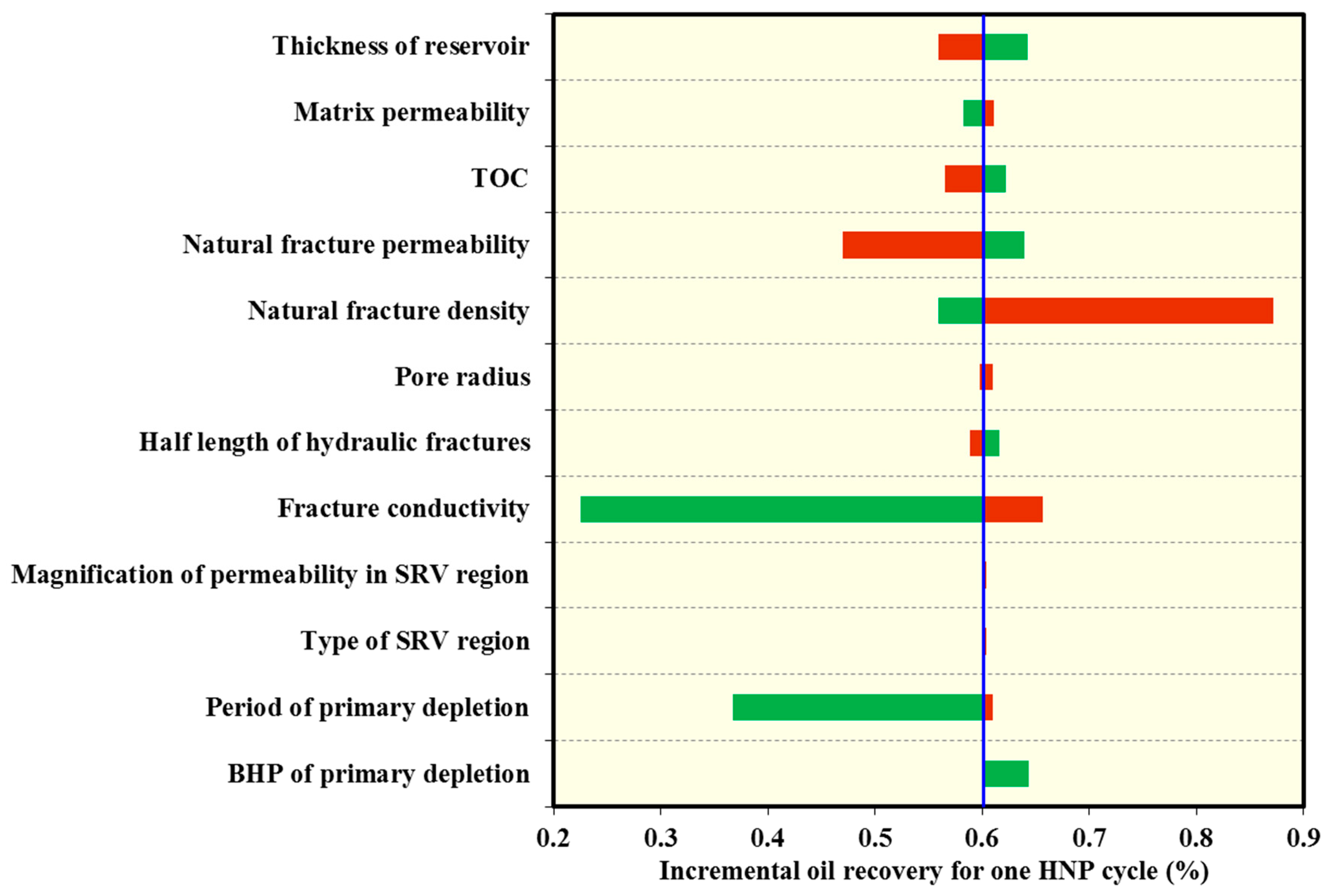
Figure 31.
Tornado chart indicating the most and least sensitive parameters for incremental oil recovery. Each green bar corresponds to a sensitivity measure (compared to a base case) when a parameter is set to its lower bound. The red bars are for the upper bounds. The vertical blue line denotes the base case.
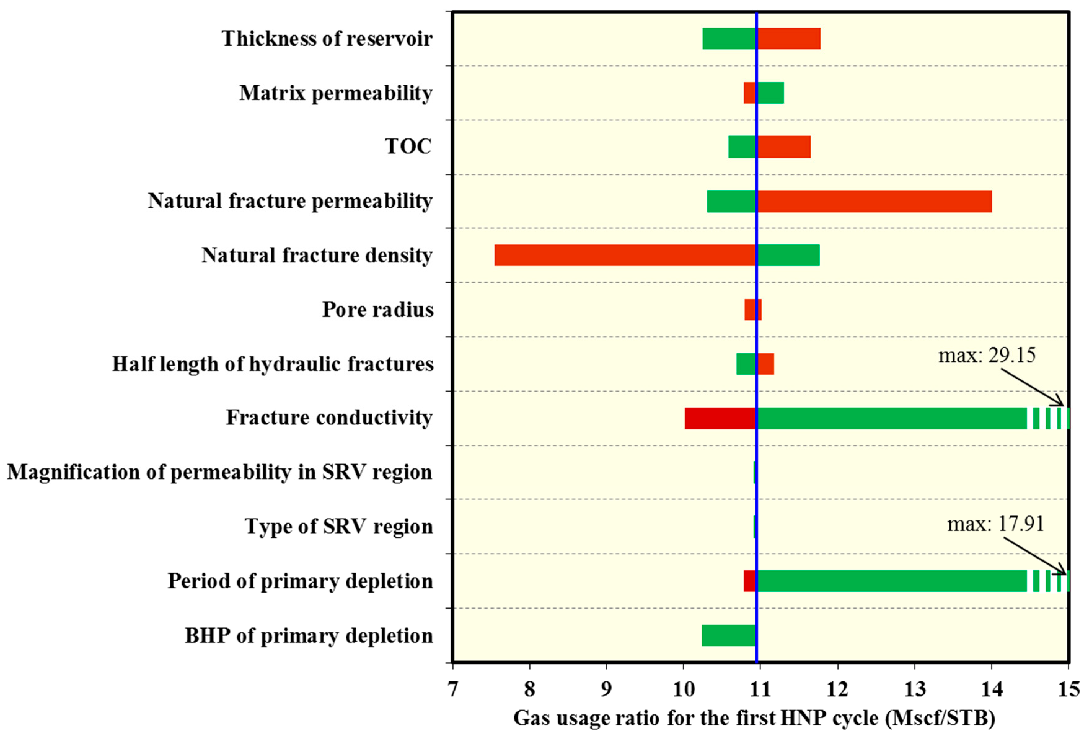
Figure 32.
Tornado chart indicating the most and least sensitive parameters for gas usage ratio. Each green bar corresponds to a sensitivity measure (compared to a base case) when a parameter is set to its lower bound. The red bars are for the upper bounds. The vertical blue line denotes the base case.
Table 1.
Compositional data for the Duvernay volatile oil well.
Table 1.
Compositional data for the Duvernay volatile oil well.
| Component | Molar
Fraction | Critical
Pressure [atm] | Critical
Temperature [K] | Critical Volume
[L/mol] | Molar Weight
[g/gmol] | Acentric
Factor | Parachor
Coefficient |
|---|
| N2 | 0.0026 | 33.50 | 126.20 | 0.0895 | 28.01 | 0.0400 | 41.00 |
| CO2 | 0.0053 | 72.80 | 304.20 | 0.0940 | 44.01 | 0.2250 | 78.00 |
| CH4 | 0.5403 | 45.40 | 190.60 | 0.0990 | 16.04 | 0.0080 | 77.00 |
| C2H6 | 0.1260 | 48.20 | 305.40 | 0.1480 | 30.07 | 0.0980 | 108.00 |
| C3H8 | 0.0764 | 41.90 | 369.80 | 0.2030 | 44.10 | 0.1520 | 150.30 |
| C4 | 0.0480 | 37.06 | 427.62 | 0.2058 | 23.81 | 0.2344 | 187.47 |
| C5–C6 | 0.0522 | 33.00 | 507.00 | 0.1222 | 77.57 | 0.2500 | 237.58 |
| C7+ | 0.1492 | 20.28 | 655.58 | 0.7073 | 157.30 | 0.4882 | 484.01 |
Table 2.
Binary interaction parameters for the Duvernay volatile oil well.
Table 2.
Binary interaction parameters for the Duvernay volatile oil well.
| Component | N2 | CO2 | CH4 | C2H6 | C3H8 | C4 | C5–C6 | C7+ |
|---|
| N2 | 0.0000 | −0.0200 | 0.0310 | 0.0420 | 0.0910 | 0.0950 | 0.1100 | 0.1300 |
| CO2 | −0.0200 | 0.0000 | 0.1200 | 0.1100 | 0.1000 | 0.1200 | 0.1250 | 0.1400 |
| CH4 | 0.0310 | 0.1200 | 0.0000 | 0.0040 | 0.0128 | 0.0133 | 0.0011 | 0.0906 |
| C2H6 | 0.0420 | 0.1100 | 0.0040 | 0.0000 | 0.0025 | 0.0027 | 0.0009 | 0.0587 |
| C3H8 | 0.0910 | 0.1000 | 0.0128 | 0.0025 | 0.0000 | 0.0000 | 0.0064 | 0.0379 |
| C4 | 0.0950 | 0.1200 | 0.0133 | 0.0027 | 0.0000 | 0.0000 | 0.0068 | 0.0371 |
| C5–C6 | 0.1100 | 0.1250 | 0.0011 | 0.0009 | 0.0064 | 0.0068 | 0.0000 | 0.0732 |
| C7+ | 0.1300 | 0.1400 | 0.0906 | 0.0587 | 0.0379 | 0.0371 | 0.0732 | 0.0000 |
Table 3.
Critical properties of the eight pseudocomponents corresponding to different pore radius in Duvernay volatile oil well.
Table 3.
Critical properties of the eight pseudocomponents corresponding to different pore radius in Duvernay volatile oil well.
| Component | Bulk Phase | rp = 10 nm | rp = 30 nm | rp = 50 nm | rp = 2000 nm |
|---|
| Pc [atm] | Tc [K] | Pc [atm] | Tc [K] | Pc [atm] | Tc [K] | Pc [atm] | Tc [K] | Pc [atm] | Tc [K] |
|---|
| N2 | 33.50 | 126.20 | 32.31 | 121.74 | 33.10 | 124.70 | 33.26 | 125.30 | 33.49 | 126.18 |
| CO2 | 72.80 | 304.20 | 70.14 | 293.06 | 71.91 | 300.46 | 72.26 | 301.95 | 72.79 | 304.14 |
| CH4 | 45.40 | 190.60 | 43.74 | 183.61 | 44.84 | 188.25 | 45.06 | 189.19 | 45.39 | 190.56 |
| C2H6 | 48.20 | 305.40 | 46.18 | 292.58 | 47.52 | 301.09 | 47.79 | 302.81 | 48.19 | 305.34 |
| C3H8 | 41.90 | 369.80 | 39.94 | 352.48 | 41.24 | 363.98 | 41.50 | 366.30 | 41.89 | 369.71 |
| C4 | 37.06 | 427.62 | 35.16 | 405.75 | 36.42 | 420.26 | 36.67 | 423.19 | 37.05 | 427.51 |
| C5–C6 | 33.00 | 507.00 | 31.15 | 478.51 | 32.38 | 497.40 | 32.62 | 501.23 | 32.99 | 506.86 |
| C7+ | 20.28 | 655.58 | 18.83 | 608.59 | 19.79 | 639.70 | 19.99 | 646.03 | 20.28 | 655.34 |
Table 4.
Diffusion coefficients of different components.
Table 4.
Diffusion coefficients of different components.
| Component | Diffusion Coefficient [cm2/s] |
|---|
| N2 | 0.008000 |
| CO2 | 0.007692 |
| CH4 | 0.01000 |
| C2H6 | 0.007692 |
| C3H8 | 0.003846 |
| C4 | 0.001282 |
| C5+ | 0.000256 |
Table 5.
Basic reservoir and fracture properties used for history matching.
Table 5.
Basic reservoir and fracture properties used for history matching.
| Parameters | Value | Unit |
|---|
| Model dimension | 2600 × 610 × 45 | m |
| Number of grid blocks | 260 × 61 × 9 | – |
| Grid cell dimension | 10 × 10 × 5 | m |
| Initial reservoir pressure | 63.8 | MPa |
| Reservoir temperature | 255 | °F |
| Reservoir depth | 3450 | m |
| Reservoir porosity | 0.035 | – |
| Matrix permeability | 0.0002 | mD |
| Matrix water saturation | 0.17 | – |
| Fracture height | 26.52 | m |
| Fracture half-length | 60 | m |
| Fracture conductivity | 100 | mD.cm |
| Fracture water saturation | 0.49 | – |
| Fracture width | 0.4 | m |
Table 6.
Summary of geological and engineering parameters for the simulation.
Table 6.
Summary of geological and engineering parameters for the simulation.
| Type | Parameter | Unit | Range | Base Case |
|---|
| Reservoir | Thickness of reservoir | m | 15, 30, 45, 60, 75 | 45 |
| TOC | | 2%, 4%, 6%, 10% | 4% |
| Pore radius | nm | 10, 30, 50, 2000 | 10 |
| Matrix permeability | mD | 5∙10−5, 1∙10−4, 2∙10−4, 5∙10−4 | 2∙10−4 |
| Natural fracture density | NO. of fractures/m | None, 0.05, 0.1, 0.2, 0.5 | 0.1 |
| Natural fracture permeability | mD | 0.0005, 0.001, 0.002, 0.005 | 0.001 |
| Hydraulic fracturing | Half-length of hydraulic fractures | m | 35, 60, 85 | 60 |
| Fracture conductivity | mD·cm | 10, 100, 1000, 10,000 | 100 |
| Type of stimulated reservoir volume (SRV) region | | A, B, C, D | C |
| Magnification of permeability in SRV region | | 1, 2, 5, 8 | 2 |
| Primary Depletion | Period of primary depletion | year | 1, 3, 5, 7 | 5 |
| BHP of primary depletion | MPa | 35, 40, 45, 50 | 45 |
Table 7.
Summary of results for huff-n-puff with different reservoir thickness.
Table 7.
Summary of results for huff-n-puff with different reservoir thickness.
| Thickness of Reservoir (m) | 15 | 30 | 45 | 60 | 75 |
|---|
| Oil rate after 5 years primary depletion (bbl/d) | 16.42 | 33.09 | 50.07 | 67.49 | 85.23 |
| Cumulative oil production for primary depletion (Mbbl) | 89.51 | 177.11 | 262.52 | 345.53 | 426.03 |
| Cumulative volume of injected gas for first huff-n-puff cycle (MMscf) | 58.83 | 117.67 | 176.50 | 235.33 | 294.17 |
| Cumulative oil production with one huff-n-puff cycle (Mbbl) | 95.26 | 188.31 | 278.62 | 366.17 | 451.01 |
| Duration of the first huff-n-puff cycle (d) | 325 | 365 | 400 | 435 | 465 |
| Gas usage ratio for the first huff-n-puff cycle (Mscf/STB) | 10.25 | 10.50 | 10.96 | 11.40 | 11.78 |
| Incremental oil recovery for the first huff-n-puff cycle (%) | 0.64 | 0.63 | 0.60 | 0.58 | 0.56 |
Table 8.
Summary of results for huff-n-puff with different TOC.
Table 8.
Summary of results for huff-n-puff with different TOC.
| TOC (%) | 2 | 4 | 6 | 10 |
|---|
| Oil rate after 5 years primary depletion (bbl/d) | 46.61 | 50.07 | 52.77 | 57.36 |
| Cumulative oil production for primary depletion (Mbbl) | 255.65 | 282.55 | 303.71 | 340.01 |
| Cumulative volume of injected gas for first huff-n-puff cycle (MMscf) | 176.50 | 176.50 | 176.50 | 176.50 |
| Cumulative oil production with one huff-n-puff cycle (Mbbl) | 272.33 | 298.65 | 319.46 | 355.16 |
| Duration of the first huff-n-puff cycle (d) | 380 | 400 | 415 | 441 |
| Gas usage ratio for the first huff-n-puff cycle (Mscf/STB) | 10.58 | 10.96 | 11.21 | 11.65 |
| Incremental oil recovery for the first huff-n-puff cycle (%) | 0.62 | 0.60 | 0.59 | 0.56 |
Table 9.
Summary of results for huff-n-puff with different pore radius of shale matrix.
Table 9.
Summary of results for huff-n-puff with different pore radius of shale matrix.
| Pore Radius of Shale Matrix (nm) | 10 | 30 | 50 | 2000 |
|---|
| Oil rate after 5 years primary depletion (bbl/d) | 50.07 | 49.06 | 48.87 | 48.62 |
| Cumulative oil production for primary depletion (Mbbl) | 282.55 | 275.66 | 274.05 | 272.03 |
| Cumulative volume of injected gas for first huff-n-puff cycle (MMscf) | 176.50 | 176.50 | 176.50 | 176.50 |
| Cumulative oil production with one huff-n-puff cycle (Mbbl) | 298.65 | 291.69 | 290.25 | 288.39 |
| Duration of the first huff-n-puff cycle (d) | 400 | 400 | 395 | 395 |
| Gas usage ratio for the first huff-n-puff cycle (Mscf/STB) | 10.96 | 11.01 | 10.89 | 10.79 |
| Incremental oil recovery for the first huff-n-puff cycle (%) | 0.60 | 0.60 | 0.60 | 0.61 |
Table 10.
Summary of results for huff-n-puff with different matrix permeability.
Table 10.
Summary of results for huff-n-puff with different matrix permeability.
| Matrix Permeability (mD) | 5∙10−5 | 1∙10−4 | 2∙10−4 | 5∙10−4 |
|---|
| Oil rate after 5 years primary depletion (bbl/d) | 47.36 | 48.06 | 50.07 | 56.30 |
| Cumulative oil production for primary depletion (Mbbl) | 250.78 | 255.36 | 262.52 | 281.21 |
| Cumulative volume of injected gas for first huff-n-puff cycle (MMscf) | 176.50 | 176.50 | 176.50 | 176.50 |
| Duration of the first huff-n-puff cycle (d) | 555 | 465 | 400 | 355 |
| Cumulative oil production with one huff-n-puff cycle (Mbbl) | 292.68 | 293.62 | 298.65 | 317.57 |
| Gas usage ratio for the first huff-n-puff cycle (Mscf/STB) | 11.31 | 11.09 | 10.96 | 10.78 |
| Incremental oil recovery for the first huff-n-puff cycle (%) | 0.58 | 0.59 | 0.60 | 0.61 |
Table 11.
Summary of results for huff-n-puff with different natural fracture density.
Table 11.
Summary of results for huff-n-puff with different natural fracture density.
| Natural Fracture Density (NO. of Fractures/m) | Without | 0.05 | 0.1 | 0.2 | 0.5 |
|---|
| Oil rate after 5 years primary depletion (bbl/d) | 21.64 | 50.76 | 50.07 | 49.82 | 49.63 |
| Cumulative oil production for primary depletion (Mbbl) | 177.20 | 283.82 | 282.55 | 283.39 | 283.03 |
| Cumulative volume of injected gas for first huff-n-puff cycle (MMscf) | 176.50 | 176.50 | 176.50 | 176.50 | 176.50 |
| Cumulative oil production with one huff-n-puff cycle (Mbbl) | 196.45 | 298.82 | 298.65 | 302.52 | 306.42 |
| Duration of the first huff-n-puff cycle (d) | 765 | 445 | 400 | 420 | 425 |
| Gas usage ratio for the first huff-n-puff cycle (Mscf/STB) | 9.17 | 11.76 | 10.96 | 9.23 | 7.55 |
| Incremental oil recovery for the first huff-n-puff cycle (%) | 0.72 | 0.56 | 0.60 | 0.71 | 0.87 |
Table 12.
Summary of results for huff-n-puff with different natural fracture permeability.
Table 12.
Summary of results for huff-n-puff with different natural fracture permeability.
| Natural Fracture Permeability (mD) | 0.0005 | 0.001 | 0.002 | 0.005 |
|---|
| Oil rate after 5 years primary depletion (bbl/d) | 37.99 | 50.07 | 68.62 | 100.64 |
| Cumulative oil production for primary depletion (Mbbl) | 242.13 | 282.55 | 342.14 | 453.72 |
| Cumulative volume of injected gas for first huff-n-puff cycle (MMscf) | 176.50 | 176.50 | 176.50 | 176.50 |
| Cumulative oil production with one huff-n-puff cycle (Mbbl) | 259.27 | 298.65 | 357.25 | 466.32 |
| Duration of the first huff-n-puff cycle (d) | 453 | 400 | 355 | 285 |
| Gas usage ratio for the first huff-n-puff cycle (Mscf/STB) | 10.30 | 10.96 | 11.68 | 14.01 |
| Incremental oil recovery for the first huff-n-puff cycle (%) | 0.64 | 0.60 | 0.56 | 0.47 |
Table 13.
Summary of results for huff-n-puff with different half-length of hydraulic fractures.
Table 13.
Summary of results for huff-n-puff with different half-length of hydraulic fractures.
| Half-Length of Hydraulic Fractures (m) | 35 | 60 | 85 |
|---|
| Oil rate after 5 years primary depletion (bbl/d) | 48.12 | 50.07 | 52.08 |
| Cumulative oil production for primary depletion (Mbbl) | 230.20 | 282.55 | 330.03 |
| Cumulative volume of injected gas for first huff-n-puff cycle (MMscf) | 176.50 | 176.50 | 176.50 |
| Cumulative oil production with one huff-n-puff cycle (Mbbl) | 246.72 | 298.65 | 345.83 |
| Duration of the first huff-n-puff cycle (d) | 385 | 400 | 425 |
| Gas usage ratio for the first huff-n-puff cycle (Mscf/STB) | 10.68 | 10.96 | 11.17 |
| Incremental oil recovery for the first huff-n-puff cycle (%) | 0.62 | 0.60 | 0.59 |
Table 14.
Summary of results for huff-n-puff with different fracture conductivity.
Table 14.
Summary of results for huff-n-puff with different fracture conductivity.
| Fracture Conductivity (mD·cm) | 10 | 100 | 1000 | 10,000 |
|---|
| Oil rate after 5 years primary depletion (bbl/d) | 55.35 | 50.07 | 49.19 | 49.00 |
| Cumulative oil production for primary depletion (Mbbl) | 206.33 | 282.55 | 287.19 | 287.73 |
| Cumulative volume of injected gas for first huff-n-puff cycle (MMscf) | 176.50 | 176.50 | 176.50 | 176.50 |
| Cumulative oil production with one huff-n-puff cycle (Mbbl) | 212.38 | 298.65 | 304.75 | 305.35 |
| Duration of the first huff-n-puff cycle (d) | 575 | 400 | 265 | 253 |
| Gas usage ratio for the first huff-n-puff cycle (Mscf/STB) | 29.15 | 10.96 | 10.05 | 10.02 |
| Incremental oil recovery for the first huff-n-puff cycle (%) | 0.23 | 0.60 | 0.65 | 0.66 |
Table 15.
Summary of results for huff-n-puff with different types of SRV region.
Table 15.
Summary of results for huff-n-puff with different types of SRV region.
| Type of SRV Region | A | B | C | D |
|---|
| Oil rate after 5 years primary depletion (bbl/d) | 50.01 | 50.01 | 50.07 | 50.01 |
| Cumulative oil production for primary depletion (Mbbl) | 279.19 | 278.92 | 282.55 | 278.75 |
| Cumulative volume of injected gas for first huff-n-puff cycle (MMscf) | 176.50 | 176.50 | 176.50 | 176.50 |
| Cumulative oil production with one huff-n-puff cycle (Mbbl) | 295.37 | 295.02 | 298.65 | 294.91 |
| Duration of the first huff-n-puff cycle (d) | 415 | 405 | 400 | 395 |
| Gas usage ratio for the first huff-n-puff cycle (Mscf/STB) | 10.90 | 10.97 | 10.96 | 10.92 |
| Incremental oil recovery for the first huff-n-puff cycle (%) | 0.60 | 0.60 | 0.60 | 0.60 |
Table 16.
Summary of results for huff-n-puff with different permeability magnifications in the SRV region.
Table 16.
Summary of results for huff-n-puff with different permeability magnifications in the SRV region.
| Magnification of Permeability in SRV Region | 1× | 2× | 5× | 8× |
|---|
| Oil rate after 5 years primary depletion (bbl/d) | 50.01 | 50.07 | 50.19 | 50.07 |
| Cumulative oil production for primary depletion (Mbbl) | 279.19 | 282.55 | 285.31 | 286.18 |
| Cumulative volume of injected gas for first huff-n-puff cycle (MMscf) | 176.50 | 176.50 | 176.50 | 176.50 |
| Cumulative oil production with one huff-n-puff cycle (Mbbl) | 295.37 | 298.65 | 301.40 | 302.37 |
| Duration of the first huff-n-puff cycle (d) | 415 | 400 | 392 | 392 |
| Gas usage ratio for the first huff-n-puff cycle (Mscf/STB) | 10.90 | 10.96 | 10.97 | 10.90 |
| Incremental oil recovery for the first huff-n-puff cycle (%) | 0.60 | 0.60 | 0.60 | 0.60 |
Table 17.
Summary of results for huff-n-puff with different primary depletion periods.
Table 17.
Summary of results for huff-n-puff with different primary depletion periods.
| Period of Primary Depletion (Year) | 1 | 3 | 5 | 7 |
|---|
| Oil rate after 5 years primary depletion (bbl/d) | 154.73 | 66.42 | 50.07 | 42.39 |
| Cumulative oil production for primary depletion (Mbbl) | 176.99 | 241.33 | 282.55 | 314.41 |
| Cumulative volume of injected gas for first huff-n-puff cycle (MMscf) | 176.50 | 176.50 | 176.50 | 176.50 |
| Cumulative oil production with one huff-n-puff cycle (Mbbl) | 186.85 | 256.60 | 298.65 | 330.78 |
| Duration of the first huff-n-puff cycle (d) | 150 | 320 | 400 | 440 |
| Gas usage ratio for the first huff-n-puff cycle (Mscf/STB) | 17.91 | 11.56 | 10.96 | 10.78 |
| Incremental oil recovery for the first huff-n-puff cycle (%) | 0.37 | 0.57 | 0.60 | 0.61 |
Table 18.
Summary of results for huff-n-puff with different bottom hole pressure (BHP) of primary depletion.
Table 18.
Summary of results for huff-n-puff with different bottom hole pressure (BHP) of primary depletion.
| BHP of Primary Depletion (MPa) | 35 | 40 | 45 | 50 |
|---|
| Oil rate after 5 years primary depletion (bbl/d) | 81.08 | 65.10 | 50.07 | 35.98 |
| Cumulative oil production for primary depletion (Mbbl) | 469.09 | 371.61 | 282.55 | 201.11 |
| Cumulative volume of injected gas for first huff-n-puff cycle (MMscf) | 176.50 | 176.50 | 176.50 | 176.50 |
| Cumulative oil production with one huff-n-puff cycle (Mbbl) | 486.34 | 388.52 | 298.65 | 217.22 |
| Duration of the first huff-n-puff cycle (d) | 425 | 413 | 400 | 405 |
| Gas usage ratio for the first huff-n-puff cycle (Mscf/STB) | 10.23 | 10.44 | 10.96 | 10.96 |
| Incremental oil recovery for the first huff-n-puff cycle (%) | 0.64 | 0.63 | 0.60 | 0.60 |
Table 19.
Screening criteria for gas huff-n-puff potential area in Duvernay shale volatile oil reservoirs.
Table 19.
Screening criteria for gas huff-n-puff potential area in Duvernay shale volatile oil reservoirs.
| Sensitivity Order | Parameter | Screening Criteria |
|---|
| 1 | Fracture conductivity | ≥100 mD·cm |
| 2 | Natural fracture density | ≥0.1 fracture/m |
| 3 | Period of primary depletion | ≥5 years |
| 4 | Natural fracture permeability | High value is preferable and more injected gas is needed for high permeability. |
| 5 | Reservoir thickness | ≥30 m |
| 6 | TOC | High value is preferable. |
| 7 | Matrix permeability | ≥5∙10−5 mD |
| 8 | Half-length of hydraulic fractures | Variable. Long half-length needs to inject more gas. |


 ,
, 


