Abstract
In this study, the non-intrusive embedded discrete fracture model (EDFM) in combination with the Oda method are employed to characterize natural fracture networks fast and accurately, by identifying the dominant water flow paths through spatial connectivity analysis. The purpose of this study is to present a successful field case application in which a novel workflow integrates field data, discrete fracture network (DFN), and production analysis with spatial fracture connectivity analysis to characterize dominant flow paths for water intrusion in a field-scale numerical simulation. Initially, the water intrusion of single-well sector models was history matched. Then, resulting parameters of the single-well models were incorporated into the full field model, and the pressure and water breakthrough of all the producing wells were matched. Finally, forecast results were evaluated. Consequently, one of the findings is that wellbore connectivity to the fracture network has a considerable effect on characterizing the water intrusion in fractured gas reservoirs. Additionally, dominant water flow paths within the fracture network, easily modeled by EDFM as effective fracture zones, aid in understanding and predicting the water intrusion phenomena. Therefore, fracture clustering as shortest paths from the water contacts to the wellbore endorses the results of the numerical simulation. Finally, matching the breakthrough time depends on merging responses from multiple dominant water flow paths within the distributions of the fracture network. The conclusions of this investigation are crucial to field modeling and the decision-making process of well operation by anticipating water intrusion behavior through probable flow paths within the fracture networks.
1. Introduction
Assessment for water control management is critical to efficiently develop naturally fractured gas reservoirs whose wells’ economic production lifespan is influenced by the water invasion into the wellbores. Naturally fractured reservoirs contain almost 40% of the global gas reserves [1], and it is well known that the performance of gas wells can significantly degrade when water intrusion is present since fractures increase the anisotropic permeability ratio. In this sense, the communication between the wellbore and the gas–water contact is facilitated, which might lead to early excessive water production [2,3,4]. Furthermore, water intrusion can occur through several mechanisms such as water coning, water fingering, and/or water channeling through high permeability layers or fractures that connect the water zone to the wellbore. Therefore, due to the fact that fractured reservoirs are prone to premature water cut production at the early stage of recovery, modeling water intrusion phenomena plays a vital role on these reservoirs to maximize their recovery and anticipate cost-effective treatment solutions in order not only to prevent the water to bypass resources but also to avoid adding unnecessary costs regarding well workover and excessive water production, its processing, and reinjection.
In a fractured reservoir, controlling water intrusion is challenging due to the complexity that originates from a large number of uncertain variables associated with the representativity of the natural fractures’ attributes and spatial distributions. These water intrusion occurrences have been observed and evaluated for a long time by many studies [4,5,6,7,8,9]. Sheng et al. [4] present a parametric study that analyses the effect of matrix and fracture permeability, well penetration, vertical anisotropy, aquifer size and gas rate production on water intrusion. Namani et al. [5] evaluate other parameters such as net pay, fracture orientation, mobility ratio, storativity on not only excessive water production but water breakthrough times also. Abdel [6] includes the capillary pressure effect on a multiphase numerical model to evaluate coning behavior. Other studies [7,8,9] expose water production control techniques to overcome water intrusion. In that sense, water coning represents the major contributor to high water cut in fractured reservoirs. Despite the well-known fact that the water coning phenomenon takes place due to the imbalance between viscous and gravitational forces near the wellbore [10], this phenomenon adds great complexity to the model and predicts water breakthrough behavior in fractured subsurface systems. Similarly, the rapid movement of water flow through the fractures makes controlling the water influx in fractured reservoirs more challenging. Past research has stipulated that the vertical natural fracture density is the governing criterion for water breakthrough [11]. Another parameter in relation to the fracture network that has been appraised and has an impact on the water intrusion corresponds to the well trajectory. Different studies concluded that horizontal wells are less susceptible to water intrusion than vertical wells, and thereby, water breakthrough may be delayed in fractured formations [8,12,13]. However, this concept might be subject to further analysis to avoid fracture data sampling bias from the fracture network. Furthermore, general assumptions observed in water–oil systems have been applied to the study of gas reservoirs. Notwithstanding, there exist several simulation studies for modeling and understanding water intrusion in gas [4,5,8,14], the influence of natural fractures attributes has been obviated in the field-scale while focusing only on the effective fracture permeability quantification of these systems. Natural fractures can significantly affect the well performance if water intrusion occurs. Therefore, a better understanding of the driven interaction of water intrusion with natural fracture networks plays an important role in developing gas fractured reservoirs.
Currently, the availability of information related to natural fractures invites the use of stochastic-driven approaches for unveiling some of their uncertainties in naturally fractured reservoirs. However, the prediction of water and/or gas breakthrough is very challenging in such reservoirs [15], unless advanced numerical reservoir simulation is employed to accurately model the physics behind their behavior dynamics such as the water intrusion phenomenon. Yet, physics-based reservoir simulation can provide misleading results if the complexity of natural fracture configurations is not well described. Since 1998, the discrete fracture network (DFN) has become a standard geologically driven mathematical representation of fracture systems in 3D geometry [16]. Through this, fractures are modeled as planar objects with orientation, approximated dimensions, and spatial distribution. The value of DFNs relies on keeping their fracture properties unaltered after upscaling them to grid cells for posterior use as input in dynamic reservoir simulation. In that sense, common-use reservoir fracture frameworks such local grid refinement (LGR) or unstructured gridding methods make it unfeasible to model numerous fractures explicitly due to their very high computational-resource demand. Instead, the conventional methodology to model these natural fracture networks in a reservoir scale has been to upscale to dual porosity dual permeability (DPDK) frameworks [17,18,19,20,21] through the Oda or tensor method. Although the Oda method is efficient in terms of processing speed, it lacks precision as it assumes long and highly connected fractures [21,22,23,24,25,26]. Likewise, the tensor method is too slow to be applicable to full-field scale characterization [21]. On the other hand, an evolving non-intrusive method, the embedded discrete fracture model (EDFM), can model natural fractures with great reliability, flexibility, and simulation run time as exposed in different studies [27,28,29,30]. As a consequence, combining EDFM in conjunction with upscaling frameworks will overcome the limitations of existing methods and standard industrial practices [31] and generate a representative natural fracture network characterization.
In this study, we introduced an unusual feature of EDFM modeling to perform fracture spatial connectivity analysis within the DFN to screen probable water flow paths from the gas–water contact to the wellbore. The main value of this work is to model these dominant fracture trails by employing the non-intrusive EDFM technology in conjunction with a reservoir simulator as a solution to characterize a region of a gas field with water production from multiple wells efficiently. This research starts by merging DFN and geological static model to generate reservoir single-well models whose field production will be history matched. In order to achieve representative realizations of their water intrusion phenomenon and reservoir parameters, the shortest flow paths are identified from the wellbore to the water zones in the reservoir so that the effects of the attributes of the natural fractures in describing the water intrusion are preserved and validated. Subsequently, we extend the parameters of the history-matched single-well models to a field model scale with five producing wells to achieve a global history match. Next, 20-year production forecasting is performed. Finally, the effects of the dominant shortest paths within the DFN on the pressure and water saturation distribution are discussed.
2. Methodology
Mechanisms of fluid flow through fractured formations are often very complex due to the fracture network present in these reservoirs. Despite that DPDK models upscale highly copious fracture networks into a simple structured continuum, they fail to provide accurate results when the behavior of individual fractures and their attributes are of more interest. If fractures are not connected to the network but are part of a set of the fractured reservoir, the continuum assumption is no longer valid. Additionally, the representativity of the network might be not well captured when upscaling and averaging fractures that are not consistent with the cell size [22,26]. To further overcome these issues in modeling large DFNs, the non-intrusive embedded discrete fracture model (EDFM) has been proposed [28] to fill those gaps and model dominant fractures within the network explicitly.
In this study, the proposed methodology comprises five main stages to characterize water intrusion in naturally fractured gas reservoirs (Figure 1). The workflow starts with the generation of representative DFN after synergy in a conceptual model from the static analysis of well and inter-well data. The fracture density model was established by means of constraints such as curvature body, ant body and fault distance. The DFN model was generated by using the fracture density model which resulted from the statistical data of different fractures attributes. These attributes, such as dip angle and azimuth, were determinant to define two main groups of fractures as a result of single-well image logging and outcrop analogies. Next, a similar hierarchical approach to the one presented by Li and Lee [32] is employed to classify the fractures as large or not. However, in this work, the employed criteria are different and are based only on ranking the fracture planes regarding their fracture length so that the largest fractures can be explicitly modeled by EDFM in order to speed up the simulation process and be able to identify water intrusion behaviors. Lee et al [33] demonstrated that the long fractures exhibit a more dominating influence on fluid flow than other smaller fractures. The range of the fracture lengths retrieved from seismic interpretation was considered in order to define a minimum threshold dimension for “large” fractures. After EDFM is employed for the characterization of the dominant fractures in the system, the rest of the fractures (medium and smallest) are upscaled into the matrix through the Oda method. The idea behind upscaling is that smaller fractures contribution is lumped in the effective permeability estimation After that, spatial connectivity analysis is conducted to identify the shortest water flow paths to be able to characterize the water intrusion. Later, single-well models are constructed after merging EDFM characterization with fracture upscaling in order to perform individual history matching of water breakthrough for each producing well. Finally, the simulated parameters of each single well dynamic model are integrated into a full-field scale model to perform a history match of the pressure and water intrusion.

Figure 1.
Complete workflow for characterizing water intrusion in a naturally fractured reservoir. Blue circles 1, 2, and 3a refer to conventional discrete fracture network (DFN) generation and upscaling its properties into the matrix [34]. Red circles were implemented (3b, 3b*, 4, 5) and denote the features of applying embedded discrete fracture model (EDFM) method to model dominant fractures in the reservoir explicitly. Green arrows highlight the involved process in water intrusion characterization specifically.
As a result, it is important to remark that the proposed hybrid idea is intended to focus on capturing the water intrusion phenomena observed in the field. In that sense, explicit modeling of the fractures is envisioned to identify major complex behaviors of that water intrusion, that are hardly replicated with dual continuum methods.
2.1. Embedded Discrete Fracture Model (EDFM)
Explicit modeling of the fractures through EDFM is envisioned to identify major complex behaviors of that water intrusion. EDFM employs the benefits of the dual continuum and the discrete fracture models in characterizing the flow in fractured porous medium. By using EDFM, each fracture is embedded inside the matrix grid and is discretized by the cell boundaries. Then, new cells are added to the computational domain for each fracture segment, and fluid flow between fracture and matrix grid blocks is simulated based on calculations of transmissibility through non-neighboring connections (NNCs). (See Figure 2).

Figure 2.
Schematic 3D representation of simple EDFM methodology example, which depicts how a non-orthogonal fracture is embedded in the matrix grid blocks.
In order to illustrate the NNC concept, consider a matrix block intersecting two fractures (Figure 3). In a general 3D setting, each matrix grid block is connected at maximum to six other grid blocks. However, if a block is intersected by a fracture plane, an extra connection is required to calculate the fluid transfer between matrix and fracture with the EDFM approach. These additional connections are calculated as NNC from the matrix blocks to the fracture cells (virtual new grid blocks) that are embedded. In the mass balance equation, two additional directions must be included to capture matrix-fracture interactions. Therefore, eight directions occur for this example.

Figure 3.
Example of the connections a single grid block with the non-intrusive EDFM, in which two intersecting fractures planes are confined inside a single block, and thereby, eight connections will be calculated. The red arrows show the non-neighboring connections (NNCs) between matrix block “ijk” and the fracture segments [35].
In that sense, all the parameters and operators for fluid flow that are anisotropically driven must be modified to include these extra NNC. In general, if F is assumed to be a three-dimensional vector function with components Fx, Fy, and Fz in the corresponding directions, then the definition of divergence and gradient include extra terms for every NNC and can be modified as shown below [35]:
Consequently, the mass balance equation is modified to account for matrix–fracture and fracture–fracture fluid transfers when applying the EDFM method. The final form of the mass conservation equation for single-phase fluid flow in porous media including discrete embedded fracture planes is presented as follows:
for the rock matrix (m):
and for the fracture ():
where p is pressure, is the porosity; K is the permeability as a tensor to account for a generic anisotropic case; and correspond to the density and viscosity of the fluid correspondingly. Superscripts , , and refer to the matrix, fracture i and well respectively, while subscripts denote fluid. Additionally, and are the source terms (i.e., wells) on matrix m and fracture . Finally, and represent the flux exchange between the matrix and the intersecting fracture , while represents the flux exchange from the j-th fracture to the i-th fracture on intersecting fracture–fracture planes [33].
Due to mass conservation,
In that sense, the Peaceman well model is employed to obtain the well source terms for matrix and fractures as follows:
where WI is the well productivity index, and . is the effective mobility between the well and the penetrated grid cell in the medium. and are the control volume and control area used in the discrete system for matrix and fracture, respectively.
Finally, the flux exchange terms are written as:
where T depicts the transmissibility index between each two non-neighboring elements. More details of the calculations were discussed by [27,36].
2.2. Oda Method
As part of the proposed methodology, the Oda method is employed to upscale the discrete fracture networks as a standard-industry technique. It is a statistical-based approach that estimates the permeability of a fracture network based on the total area of fractures in every cell. In this paper, we will use the term Oda method to both the original and the correction approach. Oda [37] assumed penny shaped fractures. The expression is derived on the assumption of steady-state flow in the fractures using Darcy’s law based on a parallel plate setting. In particular, Oda’s method employs probability density function (PDF) which is normalized over a unit sphere as a function of fracture orientation, surface area, and aperture to account for the number of fractures in the domain of interest (fractured cell).
where is the total number of fractures, is the PDF mentioned earlier, n represents the orientation of normalized fractures over the surface of a hemisphere, is the surface of a hemisphere, a is the aperture, and r is the radius of fractures.
Hence, Oda upscaling method is described as the following expression:
where is the diagonal permeability tensor, represents the principal directions of permeability, is the Kronecker delta (which normalizes the fracture geometry over the surface of a grid cell), and represents the fracture geometry as the average void volume of fractures weighted over the volume of the grid cell.
The Oda-corrected method includes a connectivity factor (C) and a correction for fracture length (M), so that the permeability estimation is calculated by:
where , and an additional factor C0 defines a percolation threshold. More details are described by Haridy et al. [26].
2.3. Shortest Path for Water Intrusion
The most representative DFN is subject to a spatial connectivity analysis that is focused on finding the shortest path within the DFN between two explicit fracture connections. This feature aids to calibrate specific dominant fracture properties to mimic the dynamic behavior of the wells (production and water intrusion). In this workflow, the proposed routine for this connectivity analysis is intended to determine the shortest fracture paths that trigger water intrusion phenomena between the wellbore and the gas–water contact in the reservoir.
This novel feature of fracture geometrical connectivity analysis calculates the shortest Euclidean distances between fracture–fracture intersections within the fracture network, and thereby, multiple shortest paths can be screened from the whole DFN. Figure 4 shows a schematic representation of the shortest path concept (stripped lines) for identifying dominant connected water flow trail (solid lines) within the DFN from the multiple source points on the wellbore to the water zone contact.

Figure 4.
Schematic portrait of how connected fractured paths (solid lines) from the wellbore to the water zone contact network are intended to be identified within a DFN based on the shortest distance (stripped lines) in order to characterize water intrusion.
Computations for the connectivity analysis may be carried out via conventional methodologies [38]. For example, it is implemented by using an algorithm described by Yen’s algorithm for multiple shortest paths, adapted to find the shortest distances from the wellbore to the water zone using the natural fractures in a reservoir as the flow medium [39]. For instance, the applicable algorithm first identifies the shortest path from the initial node (wellbore) to the end node (water contact) (e.g., using Dijkstra’s algorithm) [40], and then iteratively finds subsequent different shortest paths in the fracture network. As a consequence, this novel workflow achieves to characterize water intrusion within a DFN explicitly on each fracture modeled by EDFM since it is the first time those algorithms are applied to identify water flow paths based on their shortest distance to the water contact after connectivity analysis within the DFN. The results are validated with posterior history matching of the observed field production through a commercial numerical reservoir simulator.
3. Field Application for Water Intrusion Characterization
3.1. General Reservoir Model Concept
The water intrusion characterization, proposed above, is applied to a region of a naturally fractured carbonate gas reservoir in Central Asia. The studied area will be named as B-P gas field and belongs to an anticlinal structure complicated by faults. The fault types are mainly strike-slip in the near east-west and north-west directions and thrust (reverse) faults in the near north-east direction. The extension length of the thrust fault is smaller, and the fault distance is larger. For this reason, the fault distance of reverse faults will have a greater impact on the structural surface while the strike-slip faults have a small fault distance, which, thereby, produces less impact on the structural surface (Figure 5). The natural fractures play a major role in gas production for this specific carbonate fractured gas reservoir where the fracture networks are the main outflow channel for the fluid to flow. Figure 6 denotes the field water saturation model which was interpreted for this gas reservoir.

Figure 5.
Full-field view of the structural map of the gas reservoir, subject of this study.

Figure 6.
Full-field 3D water saturation of the studied reservoir.
3.2. Regional 3D Static and Fracture Model Generation
A 3D geological model was constructed based on a progressive transition from 1D single well models, passing to a 2D geological drivers and fracture distribution analysis, to generating a 3D static and fracture model (See Figure 7). The details of the regional fracture model generation are described in detail in the next section. Fracture apertures, lengths and heights were stochastically generated based on the distribution of petrophysical properties and fractures and based on geological, structural, and seismic controls. The role of seismic data in generating the fracture model is to support the identification of large-scale fractures, also referred to as small faults. Thus, the length of these large-scale fractures (small faults) is determined mainly based on the seismic interpretation results corresponding to different directions.

Figure 7.
Progressive static model workflow employed to generate the fracture model.
3.3. Reservoir Discrete Fracture Network (DFN) Generation and Controls
From the wellbore of the vertical well B5, 232 fractures were identified using conventional open-hole logs, borehole image interpretations, outcrops, and cores (Figure 8a). We studied the fracture orientations for the major fracture sets at outcrops to be compared with the core and borehole fracture orientations of well B5. Two fracture sets were recognized in this well: EW and NW. Additionally, the fracture aperture size distributions, fracture frequencies, and fracture strains are markedly similar in both outcrop and core. The computed fracture densities for all detected fracture sets in this well are displayed in Figure 8b. The fractures are mainly concentrated between 3050 and 3150 m while a strong decrease in the fracture density is observed around 3170 m. Stereo plots of the identified fractures are depicted in Figure 9, where two fracture set characteristics can be noted by their different directions (the East-West, and North West). It can be observed that the highest fracture density corresponds to the set in the North West direction.

Figure 8.
Single well fracture analysis: (a) core of well B5 at 3170.58 m; (b) fracture density interpretation of different fracture sets for well B5.

Figure 9.
Example of Wellbore fractures spatial attributes that were identified in well B5: (a) Stereo net plot; (b) rose diagram; and (c) dip diagram.
In total, 1136 fractures were identified from 1D wellbore image logs from multiple wells in the field, whose summary of the attributes are displayed in Table 1.

Table 1.
Summary of fracture attributes observed from the wells 1D analysis.
Based on single-well fracture analysis, the DFN distribution will be defined from the volume measurements and different fracture drivers. Regarding the structural drivers, the type of fault controls the occurrence and distribution of associated fractures. The closer the fractures are to the fold hinge, the higher the fault intensity. Moreover, the extent of fracture development is controlled by the extension of the length of the fault, the size of fault distance, and the distance from fault as seen in Figure 10.

Figure 10.
Two-dimensional map of fracture structural driver of distance to the nearest fault.
Furthermore, seismic drivers include the analysis of fracture seismic attributes, such as curvature and ant tracking. The distribution of stress and strain is highly heterogeneous during the formation and evolution of the field, which determines the distribution of structural fractures associated with fold deformation as seen in Figure 11. Likewise, concerning fracture anisotropy, the ant track is a good indicator of the change in fracture density, as observed in Figure 12.

Figure 11.
Seismic drivers for B-P gas field: (a) Maximum curvature distribution; (b) Minimum curvature distribution of the studied gas field.

Figure 12.
Ant track distribution model of B-P gas field.
The identification and prediction of meso-small-scale fractures mainly rely on seismic data, and the accuracy of conventional seismic interpretation cannot meet the needs of fracture identification at this scale. In that sense, it is practical and feasible to use ant tracking technology to predict the distribution of meso-scale fractures. Ant tracking is a post-stack micro-fracture recognition technology that relies on an ant algorithm. It can effectively identify small fractures that cannot be explained by seismic events. Its basic principle is mainly based on the simulation of ant foraging behavior. This algorithm is a complex seismic attribute algorithm developed by Schlumberger, which spreads “electronic ants” in the seismic data volume by setting reasonable parameters. When the electronic ants encounter traces that meet the preset conditions, they release a signal that summons other ants to identify and track the break along the trace.
Furthermore, three lithofacies can be distinguished as a result of the petrophysical evaluation from the rock lithology. These lithofacies include high-energy, interfacial, and low-energy facies. From the statistical point of view of these different lithofacies, it can be seen that the interfacial lithofacies fractures are most developed (fracture development probability is 74%), followed by low-energy shoal lithofacies (fracture development probability is 24%), and high-energy shoal lithofacies fractures are underdeveloped (fracture development probability corresponds to 2%). This classification of the lithofacies in three categories can be clearly observed in Figure 13. However, the influence of lithofacies is relatively small, and thereby, there is no obvious correspondence between the distribution of lithofacies and fracture density faults, curvature and ant bodies have a greater influence on the density distribution of fractures and together with fracture density will be used to populate the fracture model (Figure 14).

Figure 13.
Distribution of lithofacies in B-P gas field.

Figure 14.
Fracture density model in B-P gas field.
Consequently, the full-field DFN is generated as a result of the progressive combination of multiple attributes, drivers, and well fracture intensity. The outcome of this process includes a full field DFN model with 2,792,795 fractures as depicted in Figure 15 and Figure 16. Large-scale fracture length was estimated from the lineament observed from seismic while smaller-scale fracture length was estimated using power-law scaling derived from lineament identified from seismic. Likewise, fracture apertures commonly follow power-law distributions. Additionally, fracture heights adhere to explicit elongation ratios. Finally, histograms of the fracture attributes in the DFN, related to dip angle, azimuth, fracture length, and fracture aperture, are found in Figure 17.

Figure 15.
Full-field DFN model for the entire reservoir. The red square delimits the B-P gas model employed for the following water intrusion characterization.

Figure 16.
Full field DFN model for the entire reservoir, displaying the fractures lengths. The red square delimits the B-P gas model employed for the following water intrusion characterization. As reference, every coordinate grid block is 2000 × 2000 m.

Figure 17.
Histograms of Field DFN attributes: (a) dip angle; (b) azimuth; (c) fracture length; (d) fracture aperture.
3.4. Well Group Reservoir Model
A sector model was extracted from the full-field reservoir model to apply the water intrusion characterization proposed in this study. As presented in the methodology section, we categorized the DFN fractures as large or small in order to be explicitly modeled or upscaled respectively in the numerical simulation. For instance, this sector model includes a total of about 120,000 fractures, and in order to simplify the complexity of the extensive fracture network, the largest fractures (around 10% of the whole number of fractures) were screened out and simulated explicitly by the EDFM method for better water intrusion characterization. This 10% was representative of the largest, and per se, dominant fractures as their dimensions fell within the ranges of the fractures retrieved from seismic interpretation.
A total of five gas wells (one vertical well, four large deviated wells) are included in the studied area. The actual names of the wells have been masked because of confidentiality matters. In that sense, the authors named the wells as B1, B2, B3, B4 and B5 for this study. Four of these wells produced water. For instance, wells B2, B3 and B5 exhibit obvious water production (See Figure 18). Table 2 compiles relevant information for the five-well group reservoir models.

Figure 18.
Five-well reservoir model for field application of water intrusion characterization. Water intrusion has been observed in wells B2, B3, and B5 (blue).
Table 2.
Basic reservoir properties used in the field-scale five-well group model.
3.5. Production Analysis
Based on reported field production observations, the actual water intrusion behavior is similar among wells B2, B3 and B5. As expected, the gas production volume drops significantly once the water production increases, which is associated with the accelerated water intrusion caused by the presence of natural fractures. These three wells are the main target of history matching in this study (Figure 19). Based on the history matching of each well, the fracture parameters of the single-well model are combined to simulate the water intrusion rule of the well group under the condition of well interference. Thus, by matching their pressure and water flow rates, the model and its water intrusion behavior can be validated to become representative for this area of the well group.

Figure 19.
Actual field production rates of well with water production: (a) Field gas and water production rates of well B2; (b) Field gas and water production rates of well B3; (c) Field gas and water production rates of well B5.
3.6. DFN Characterization (EDFM Application and Upscaling)
As presented in the methodology, the DFN characterization considers a hybrid modeling-concept by combining the EDFM and Oda method for different groups of fractures. This hybrid idea is intended to focus on capturing the water intrusion phenomena observed in the field in a computationally efficient manner. In that sense, explicit modeling of the fractures by EDFM is intended to identify major driver paths for water intrusion, which are hardly replicated with dual continuum methods. The criteria to upscale fractures or keep them as explicit relies on the ranking of the fracture planes by their fracture length and the choice of the largest ones. The minimum observed length of a fracture identified from seismic interpretations corresponds to 500 m, and thus, this value is employed as a threshold to determine whether a fracture is large enough. For instance, for this group model, the largest fractures represent about 10% of the entire DFN fractures. As a consequence, these fractures will be modeled using the EDFM method with a patented preprocessor as it is capable of explicitly accounting for each single fracture contribution without any artificial communication among independent fractures.
Additionally, the presented field case application includes a quite copious number of connected fractures, therefore, considering fracture connectivity as the criteria to screen whether a fracture should be explicit or not would not be too advantageous when screening fractures out since most of them are interconnected, and thereby, using that approach would involve modeling almost all of the fractures with EDFM, and consequently, using higher computational simulation resources and time.
On the other hand, the smaller fractures will be modeled by the Oda method in order to simplify the model and to speed up the simulation process. In that sense, most of the fractures (the shortest 110,000 fractures within the well group model) were upscaled into the matrix (Figure 20). The Oda method was employed to upscale the fracture attributes, so that smaller fracture contributions are lumped into the effective permeability and porosity estimation of a pseudo-matrix. Additionally, by incorporating the Oda process into DFN characterization, the contribution to the flow of the fractures is homogenized. This upscaling method aids to speed up the characterization since it is very fast and works well with similar well-connected fractures. Nevertheless, this study will enhance the representativity of the characterization of water intrusion by searching and modeling dominant fracture paths of water intrusion to each well after applying EDFM method.

Figure 20.
Scheme of the process for upscaling 110,000 well-connected fractures into the matrix.
3.7. Water Intrusion Modeling (Shortest Path Identification)
The specific workflow that was applied in this group model for identifying the shortest fracture paths for water intrusion is portraited in Figure 21. It starts by verifying the wells with water production. Then, connectivity analysis was performed to identify connected fracture planes within the DFN between two explicit fracture connections. For the sake of water intrusion analysis, these two points include one at a perforation in the well and one at the gas–water contact (−2940 m). Screening these dominant fracture paths aided to adjust their conductivity attributes to better capture the water influx into the well. Finally, multiple shortest paths will be identified along the wellbore, all of which will be tested in the dynamic simulation to mimic the trends of the production behavior of the wells.

Figure 21.
Workflow for water intrusion modeling applied in the well group model.
4. Single Well Modeling Results
Single-well models were numerically simulated with a commercial simulator using the gas flow rate as the constrain parameter to match water flow rates and bottom-hole pressure (BHP) responses. All reservoir parameters were preserved from the general reservoir model concept. The main focus on conducting the single-well modeling corresponded to capture the water intrusion response. On the other hand, BHP response would be considered as preliminary since it was going to be subject of well interference once field modeling grouped the single-well models.
4.1. History Matching of Well B3
A single-well model of B3 was generated after upscaling the fractures attributes into the matrix and modeling the dominant fractures by EDFM. For instance, the fracture screening resulted in a total of four water intrusion paths and 50 fractures (Figure 22). Sensitivities on the effect of each shortest path were performed to compare the trend of water production response of the model with the actual field water production behavior (Figure 23). For this well, only the water intrusion behavior of path 3 and path 4 are similar to the actual water intrusion laws (Figure 24). Therefore, the corresponding fractures that intersect the wellbore are retained, and the actual water production response is matched by simulating its water intrusion through these dominant fractures.

Figure 22.
Four shortest fracture paths from well B3 to the water contact: (a) 3D visualization of the fractures paths along the wellbore; (b) shortest fractures planes embedding the grid blocks displaying a vertical intersection plane view of the water saturation of the matrix.

Figure 23.
Actual water intrusion trend of well B3.

Figure 24.
Different water intrusion responses from four different paths to well B3: (a) water rate from shortest path 1; (b) water rate from shortest path 2; (c) water rate from shortest path 3; (d) water rate from shortest path 4.
As a result, for the water intrusion of well B3, the attributes of path 3 and path 4 were adjusted to increase the fracture permeability and aperture. Hence, the water breakthrough time and the volumes were controlled and fitted. The actual water intrusion behavior of B3 single-well model is matched by the mutual influence of the two paths after quick calibration of the fracture parameters. (See Figure 25).

Figure 25.
Single-well model simulation and history matching results of well B3. The points represent the field data while the solid lines represent the simulated values: (a) gas flow rate history matching results; (b) water flow rate history matching results; (c) bottom-hole pressure (BHP) history matching results.
4.2. History Matching of Well B2
The water intrusion behavior of well B2 is similar to that of B3. The early water production of B2 is low. After almost two years of production, water intrusion in the fractures is accelerated. As a result, water production has increased significantly in conjunction with n undesired decrement in gas production. For this well, six water intrusion paths were tested, with a total of 87 fractures (Figure 26).

Figure 26.
Six shortest fracture paths from well B2 to the water contact: (a) 3D visualization of the fractures paths along the wellbore; (b) shortest fractures planes embedding the grid blocks which display a vertical intersection plane view of the water saturation of the matrix.
The simulation results appraised the water intrusion trend behavior of the six paths, all of which are consistent with the actual field water intrusion behavior (Figure 27). In fact, the water intrusion behavior of path 4 is very proximate to the actual water intrusion behavior, with some excess of water production at later time. Therefore, the water intrusion behavior of well B2 is mainly matched by adjusting the permeability and aperture of the fractures corresponding to path 4 (Figure 28).

Figure 27.
Actual field water intrusion behavior of well B2.

Figure 28.
Different water intrusion responses from six different paths to well B2.
As a result, by adjusting the fracture parameters of path 4, the simulated peak of water production and water intrusion trend is essentially in line with the actual water intrusion behavior, causing a favorable history match as seen in Figure 29.

Figure 29.
Single-well model simulation and history matching results of well B2. The points represent the field data while the solid lines represent the simulated values: (a) gas flow rate history matching results; (b) water flow rate history matching results; (c) BHP history matching results.
4.3. History Matching of Well B5
The situation of well B5 was special because it is a vertical well, whose water intrusion path is more intense. The number of fractures connecting the bottom water and the wellbore is smaller because the distance between the vertical well and the water contact is shorter than in horizontal wells, and thereby, the water breakthrough is faster. Therefore, it is necessary to reduce the fracture conductivity of the fracture near the bottom (Figure 30) in order to delay the early water production. The water intrusion behavior of the final simulation result is consistent with the actual water intrusion behavior (Figure 31).

Figure 30.
Shortest fracture paths from well B5 (vertical well) to the water contact: (a) initial shortest fracture paths; (b) bottom fractures planes (pink) in the shortest path; (c) Shortest fracture paths embedding the matrix blocks which display a vertical intersection plane view of the water saturation of the matrix.

Figure 31.
Single-well model simulation and history matching results of well B5. The points represent the field data while the solid lines represent the simulated values: (a) gas flow rate history matching results; (b) water flow rate history matching results; (c) BHP history matching results.
4.4. History Matching of Well B4
Well B4 does not exhibit significant water intrusion. It does not produce water at the early stage of production. However, this well produced only few cubic meters at later time when the water intrusion rate is fast, and the water–gas ratio increased, which might escalate in the future. In that sense, a total of eight water intrusion paths and 60 fractures are screened from the DFN (see Figure 32). After screening, the water intrusion path that does not produce water in the early stage but retains water in the later stage is retained. The water intrusion behavior of B4 is matched (see Figure 33).

Figure 32.
Six shortest fracture paths from well B4 to the water contact: (a) 3D visualization of the fractures paths along the wellbore; (b) shortest fractures planes embedding the grid blocks which display a vertical intersection 3D view of the water saturation of the matrix.

Figure 33.
Single-well model simulation and history matching results of well B4. The points represent the field data while the solid lines represent the simulated values: (a) gas flow rate history matching results; (b) water flow rate history matching results; (c) BHP history matching results.
4.5. History Matching of Well B1
Well B1 does not reported any water production. The fracture parameters were adjusted to match the pressure (Figure 34). Therefore, history matching was conducted only on the BHP response as seen in Figure 35.

Figure 34.
Shortest fracture paths to the water contact for well B1.

Figure 35.
Single-well model simulation and history matching results of well B1. The points represent the field data while the solid lines represent the simulated values: (a) gas flow rate history matching results; (b) BHP history matching results.
5. Five-Well Group Modeling Results
After matching the water intrusion behaviors of the four water-producing wells, the adjusted fracture parameters of each well are merged into the well group model. Starting from this important assumption, history matching of the well group is then performed to obtain a representative realization of the water intrusion phenomenon in a multiwell reservoir scale. The detailed work of the single-well history matching process is covered in-depth throughout this document. The relative permeability parameters and the fluid model are taken as provided by the operator of the field and their analysis is out of the scope of this paper. As a result, the flowing bottom-hole pressure was the main target to match in the well group model, since water intrusion drivers have been well assessed previously and minor changes were needed to be implemented to tune the best match. For this purpose, well group BHP means an averaged value of the BHP field measurements from all wells.
5.1. History Matching Results of Five-Well Group model
The final history match results of the multiple-well numerical model are presented in Figure 36. Hence, this final step shows how the presented workflow can model water intrusion in naturally fractured reservoirs and reinforce the reliability for accurate production management and upcoming behavior prediction of the studied region.
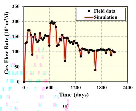

Figure 36.
Final simulation and history matching results of five-well group: (a) gas flow rate; (b) water flow rate; (c) BHP. The points represent the field data while the solid lines represent the simulated values.
5.2. Visualizations of Pressure Distributions and Water Saturation
In order to further gain insights regarding the detailed effects of the shortest paths within the natural fracture networks on the well pressure response and water intrusion phenomenon, the most straightforward method is to visualize their 3D distributions at different time steps. In Figure 37, both the pressure distributions in the matrix (left column) and fractures (right column) are plotted for the five-well group model. It is clearly observed that the pressure at the dominant fractures paths is very low, meaning severe well drainage is happening from those connected paths. In addition, the pressure communication is well portraited through the natural fractures, implying that these fractures are spatially connected and contribute to the flow of hydrocarbons.

Figure 37.
Detailed visualizations of reservoir pressure distributions in both matrix and fractures (left column) and only fractures (right columns) with five wells, more than 10,000 EDFM-fractures: (a) matrix and fractures after 270 days; (b) only fractures after 270 days; (c) matrix and fractures after 1000 days; (d) only fractures after 1000 days; (e) matrix and fractures after 1700 days; (f) only fractures after 1700 days; (g) matrix and fractures after 2000 days; (h) only fractures after 2000 days.
In Figure 38, the water saturation distributions in both matrix (left column) and fractures (right column) are depicted for the five-well group model. It is clearly observed that the water intrusion is present and arrives through the dominant fracture paths, while the water contact rises (Figure 39).

Figure 38.
Detailed visualizations of reservoir water saturation in both matrix and fractures (left column) and only fractures (right columns) with five wells, more than 10,000 EDFM-fractures: (a) matrix and fractures after 270 days; (b) only fractures after 270 days; (c) matrix and fractures after 1000 days; (d) only fractures after 1000 days; (e) matrix and fractures after 1700 days; (f) only fractures after 1700 days; (g) matrix and fractures after 2000 days; (h) only fractures after 2000 days.

Figure 39.
Detailed visualizations of the XZ plane of water saturation on the fractures with five wells and more than 10,000 EDFM-fractures. The water contact transition can be observed: (a) after 270 days; (b) after 1000 days; (c) after 1700 days; (d) after 2000 days.
6. Forecasts Simulation Results
After a satisfactory history match, production forecasts were performed based on balanced exploitation of gas fields to maintain gas production rate. This idea intends to keep the gas–water ratio of gas wells as uniform as possible to achieve a balanced lift of the gas–water contact. The advantages related to this idea are to maintain stable production, in line with the design of the development plan. On the other hand, the disadvantages are related to the fact that water production gradually increases, and the rate of growth of water production accelerates.
According to the idea of maintaining the gas production rate, the design and prediction plan for the five-well group is as follows in Table 3:
Table 3.
Details of the cases of prediction for the field-scale five-well group model.
All forecasts were simulated for 20 years controlled by pressure. The results of the forecast for each proposed case are exhibited in Figure 40. It can be clearly observed that Case 1 has the highest recovery rate in 20 years. Additionally, Case 2 and Case 1 have similar recovery levels, but Case 3 has a lower recovery rate. According to simulation results, a balanced extraction method can achieve a significant reduction in the water production of the well group, and thereby, guarantee a higher degree of recovery. Although Case 3 guarantees low water production, its gas recovery is 10 % lower, which does not meet the production needs of the operator.

Figure 40.
Comparison of the forecast results. The red solid line refers to Case 1, the blue line to Case 2, and the stripped black line to Case 3: (a) gas flow rate forecasts; (b) water flow rate forecasts; (c) as recovery factor; (d) pressure distribution after 20 years of Case 1.
Furthermore, it is important to evaluate how significant the volume of water production is that each well can deliver with respect to the global water production of the model. In that sense, for case 2, the water production ratio between the well groups is more uniform than for case 1, which can optimize the uniform water invasion between the fractures. This comparison is presented in Figure 41.

Figure 41.
Comparison of the forecasts results of water production ratio per well: (a) Case 1; (b) Case 2.
7. Conclusions
A novel workflow was applied successfully to a field case, in which water intrusion was characterized in a naturally fractured reservoir model by virtue of the identification and discrete modeling of dominant fracture paths that facilitate the water flow from the water contact for the first time. A new feature of EDFM was incorporated to address their spatial connectivity analysis of the fracture network, and thereby find the previously mentioned fracture paths. Likewise, many different methods exist for DFN characterization, each of which has its own advantages and disadvantages. However, we applied an innovative hybrid concept which combined the EDFM and Oda method to model extensive DFN networks. Our coupled model was validated with multiphase history matching of the field produced volumes. Three forecast cases were explored to determine the most suitable exploitation approach for this group of wells. The following are the detailed conclusions derived from this study:
- (1)
- By applying new algorithms that search for multiple connected fracture trails within the DFN, different paths that meet the actual water intrusion behavior can be selected by ranking their total distance. Therefore, the proposed workflow aids to simulate and quickly match the corresponding water intrusion behavior.
- (2)
- EDFM fills the gap of modeling extensive DFN, whose unconnected fractures play a significant role in the dynamics of the reservoir and create unconventional pathways, contrary to conventional upscaling methods that assume fractures are very well connected all the time.
- (3)
- Fracture conductivity and the number of fracture elements that compose a flow trail (shortest path) have a considerable effect on water intrusion in fractured gas reservoirs. As shown in this study, EDFM not only honors the fracture permeabilities, but also their attributes, geometries, orientation, distribution, and connectivity.
- (4)
- Despite the high-productivity potential of a well in a gas reservoir, the lower the gas production rate is, the lower the water cut is, which aligns with smaller pressure depletion in that region. However, if this practice is too severe, it can undermine the recovery and make it unfeasible. Therefore, the optimization of the gas production rate is crucial for controlling water intrusion phenomena by targeting the most profitable long-term economic conditions.
Author Contributions
Conceptualization, P.C. and M.F.-T.; methodology and investigation C.G., M.C. and J.L.-A.; writing—original draft preparation, P.C. and M.F.-T.; writing—review and editing, W.Y., H.X. and Z.M.; project administration, J.M. and K.S.; funding acquisition, Y.X. and H.S. All authors have read and agreed to the published version of the manuscript.
Funding
This research was funded by “National Science and Technology Major Project of China, grant number 2017ZX05030003-003-002” and “CNPC Technology Major Project, grant number 2018D-4305”.
Acknowledgments
The authors would like to acknowledge the final support from National Science and Technology Major Project of China “Water influx mechanism and development strategy of gas reservoirs with edge and bottom water” (No. 2017ZX05030003-003-002) and CNPC Technology Major Project “Oversea complex gas reservoirs fine evaluation and prediction” (No.2018D-4305). We would also like to acknowledge Sim Tech LLC for providing the EDFM software for this investigation.
Conflicts of Interest
The authors declare no conflict of interest.
Nomenclature
| A | = | Area |
| = | 3D function vector | |
| = | Number of fracture connections | |
| Kf | = | Fracture permeability |
| K | = | Element in the absolute permeability tensor |
| p | = | Pressure |
| = | Source term, | |
| = | Flux exchange | |
| = | Fracture i | |
| M | = | Matrix |
| γj | = | Specific gravity of phase j |
| δ | = | Kronecker delta, |
| λ | = | Effective mobility |
| μj | = | Viscosity of phase j |
| ρ | = | Total mass density |
| = | Reservoir matrix porosity | |
| T | = | Transmissibility |
| WI | = | Well productivity index |
| = | Total Number of fractures | |
| = | Bulk volume of a grid block | |
| n | = | The orientation of normalized fractures over the surface of a hemisphere |
| = | Surface of a hemisphere | |
| a | = | Fracture aperture |
| r | = | Radius of fractures |
| = | Diagonal permeability tensor | |
| C | = | Connectivity factor |
| Abbreviations | ||
| BHP | = | Bottomhole pressure |
| DFN | = | Discrete fracture network |
| DPDK | = | Dual porosity dual permeability |
| EDFM | = | Embedded discrete fracture model |
| G&G | = | Geophysics and geology |
| HM | = | History matching |
| LGR | = | Local grid refinement |
| NNC | = | Non-neighbor connections |
References
- Ahmed, T. Fractured Reservoirs. In Reservoir Engineering Handbook; Gulf Professional Publishing: Houston, TX, USA, 2010. [Google Scholar]
- Beattie, D.; Roberts, B. Water Coning in Naturally Fractured Gas Reservoirs. In Proceedings of the SPE Gas Technology Symposium, Calgary, AB, Canada, 28 April–1 May 1996. [Google Scholar] [CrossRef]
- Inikori, S.O. Numerical Study of Water Coning Control with Downhole Water Sink (DWS) Well Completions in Vertical and Horizontal Wells. Ph.D. Thesis, Louisiana State University, Baton Rouge, LA, USA, 2002. [Google Scholar]
- Shen, W.; Liu, X.-H.; Li, X.-Z.; Lu, J.-L. Water coning mechanism in Tarim fractured sandstone gas reservoirs. J. Central South Univ. 2015, 22, 344–349. [Google Scholar] [CrossRef]
- Namani, M.; Asadollahi, M.; Haghighi, M. Investigation of Water Coning Phenomenon in Iranian Carbonate Fractured Reservoirs. In Proceedings of the International Oil Conference and Exhibition in Mexico, Veracruz, Mexico, 27–30 June 2007. [Google Scholar] [CrossRef]
- Azim, R.A. Evaluation of water coning phenomenon in naturally fractured oil reservoirs. J. Pet. Explor. Prod. Technol. 2015, 6, 279–291. [Google Scholar] [CrossRef]
- Bedaiwi, E.; Al-Anazi, B.D.; Al-Anazi, A.F.; Paiaman, M. Polymer injection for water production control through permeability alteration in fractured reservoir. NAFTA J. 2009, 60, 221–223. [Google Scholar]
- Perez, E.; De La Garza, F.R.; Samaniego-Verduzco, F. Water Coning in Naturally Fractured Carbonate Heavy Oil Reservoir—A Simulation Study. In Proceedings of the SPE Latin America Petroleum Engineering Conference, Mexico City, Mexico, 16–18 April 2012. [Google Scholar]
- Ghosh, B.; Ali, S.A.; Belhaj, H. Controlling excess water production in fractured carbonate reservoirs: Chemical zonal protection design. J. Pet. Explor. Prod. Technol. 2020, 10, 1921–1931. [Google Scholar] [CrossRef]
- Muskat, M.; Wycokoff, R. An Approximate Theory of Water-coning in Oil Production. Trans. AIME 1935, 114, 144–163. [Google Scholar] [CrossRef]
- Van Golf-Racht, T. Water-Coning in a Fractured Reservoir. In Proceedings of the SPE Annual Technical Conference and Exhibition, New Orleans, LA, USA, 25–28 September 1994. [Google Scholar] [CrossRef]
- Dabiri, A.; Karaei, M.A.; Azdarpour, A. Simulation study of controlling water coning in oil reservoirs through drilling of horizontal wells. Biosci. Biotechnol. Res. Commun. 2017, 10, 132–136. [Google Scholar] [CrossRef]
- Razavi, O.; Vajargah, A.K.; Van Oort, E.; Aldin, M. Comprehensive analysis of initiation and propagation pressures in drilling induced fractures. J. Pet. Sci. Eng. 2017, 149, 228–243. [Google Scholar] [CrossRef]
- Belhaj, H.; Agha, K.; Nouri, A.; Butt, S.; Islam, M. Numerical and Experimental Modeling of Non-Darcy Flow in Porous Media. Proceedings of The SPE Latin American & Caribbean Petroleum Engineering Conference, Trinidad and Tobago, Spain, 27–30 April 2003. [Google Scholar] [CrossRef]
- Cottereau, N.; Garcia, M.H.; Gosselin, O.R.; Vigier, L. Effective Fracture Network Permeability: Comparative Study of Calculation Methods. In Proceedings of the SPE Europec/EAGE Annual Conference and Exhibition, Barcelona, Spain, 14–16 June 2010. [Google Scholar]
- Dershowitz, W.S.; Herda, H.H. Interpretation of fracture spacing and intensity. In Proceedings of the 33rd US. Symposium on Rock Mechanics, Santa Fe, New Mexico, 3–5 June 1992. [Google Scholar] [CrossRef]
- Warren, J.; Root, P. The Behavior of Naturally Fractured Reservoirs. Soc. Pet. Eng. J. 1963, 3, 245–255. [Google Scholar] [CrossRef]
- Kazemi, H.; Merrill, L.; Porterfield, K.; Zeman, P. Numerical Simulation of Water-Oil Flow in Naturally Fractured Reservoirs. Soc. Pet. Eng. J. 1976, 16, 317–326. [Google Scholar] [CrossRef]
- Milad, B.; Ghosh, S.; Slatt, R.M.; Marfurt, K.J.; Fahes, M. Practical Aspects of Upscaling Geocellular Geological Models for Reservoir Fluid Flow Simulations: A Case Study in Integrating Geology, Geophysics, and Petroleum Engineering Multiscale Data from the Hunton Group. Energies 2020, 13, 1604. [Google Scholar] [CrossRef]
- Milad, B.; Ghosh, S.; Suliman, M.; Slatt, R.M. Upscaled DFN models to understand the effects of natural fracture properties on fluid flow in the Hunton Group tight Limestone. In Proceedings of the Unconventional Resources Technology Conference, Houston, TX, USA, 23–25 July 2018. [Google Scholar] [CrossRef]
- Elfeel, A.M. Improved Upscaling and Reservoir Simulation of Enhanced Oil Recovery Processes in Naturally Fractured Reservoirs. Ph.D. Thesis, Heriot-Watt University, Edinburgh, UK, 2014. [Google Scholar]
- Long, J.C.S.; Witherspoon, P.A. The relationship of the degree of interconnection to permeability in fracture networks. J. Geophys. Res. Space Phys. 1985, 90, 3087. [Google Scholar] [CrossRef]
- Dershowitz, B.; Lapointe, P.; Eiben, T.; Wei, L. Integration of Discrete Feature Network Methods with Conventional Simulator Approaches. SPE Reserv. Eval. Eng. 2000, 3, 165–170. [Google Scholar] [CrossRef]
- Garcia, M.H.; Gouth, F.M.; Gosselin, O.R. Fast and Efficient Modeling and Conditioning of Naturally Fractured Reservoir Models Using Static and Dynamic Data. In Proceedings of the EUROPEC/EAGE Conference and Exhibition, London, UK, 11–14 June 2007. [Google Scholar] [CrossRef]
- Wang, H. Multiphase, Multiscale Simulation of Fractured Reservoirs. Ph.D. Thesis, University of Utah, Salt Lake, UT, USA, 2008. [Google Scholar]
- Haridy, M.G.; Sedighi, F.; Ghahri, P.; Ussenova, K.; Zhiyenkulov, M. Comprehensive Study of the Oda Corrected Permeability Upscaling Method. In Proceedings of the SPE/IATMI Asia Pacific Oil & Gas Conference and Exhibition, Bali, Indonesia, 29–31 October 2019. [Google Scholar]
- Xu, Y.; Cavalcante Filho, J.S.A.; Sepehrnoori, K.; Yu, W. Discrete-Fracture Modeling of Complex Hydraulic-Fracture Geometries in Reservoir Simulators. SPE Reserv. Evaluation Eng. 2017, 20, 403–422. [Google Scholar] [CrossRef]
- Xu, Y.; Yu, W.; Li, N.; Lolon, E.; Sepehrnoori, K. Modeling Well Performance in Piceance Basin Niobrara Formation Using Embedded Discrete Fracture Model. In Proceedings of the 2nd Unconventional Resources Technology Conference; American Association of Petroleum Geologists AAPG/Datapages, Houston, TX, USA, 23–25 July 2018. [Google Scholar]
- Xu, Y.; Yu, W.; Sepehrnoori, K. Modeling Dynamic Behaviors of Complex Fractures in Conventional Reservoir Simulators. SPE Reserv. Eval. Eng. 2019, 22, 1110–1130. [Google Scholar] [CrossRef]
- Xu, Y.; Sepehrnoori, K. Development of an Embedded Discrete Fracture Model for Field-Scale Reservoir Simulation with Complex Corner-Point Grids. SPE J. 2019, 24, 1552–1575. [Google Scholar] [CrossRef]
- Fumagalli, A.; Pasquale, L.; Zonca, S.; Micheletti, S. An upscaling procedure for fractured reservoirs with embedded grids. Water Resour. Res. 2016, 52, 6506–6525. [Google Scholar] [CrossRef]
- Li, L.; Lee, S.H. Efficient Field-Scale Simulation of Black Oil in a Naturally Fractured Reservoir Through Discrete Fracture Networks and Homogenized Media. SPE Reserv. Eval. Eng. 2008, 11, 750–758. [Google Scholar] [CrossRef]
- Lee, S.H.; Lough, M.F.; Jensen, C.L. Hierarchical modeling of flow in naturally fractured formations with multiple length scales. Water Resour. Res. 2001, 37, 443–455. [Google Scholar] [CrossRef]
- Weber, M. Challenges and solutions for modeling naturally fractured carbonates; Beicip-Franlab. In Proceedings of the SPE Workshop: From Characterization to Production—Deciphering Naturally Fractured Carbonate Reservoirs, Manama, Bahrain, 9–10 October 2019. [Google Scholar]
- Shakiba, M. Modeling and Simulation of Fluid Flow in Naturally and Hydraulically Fractured Reservoirs Using Embedded Discrete Fracture Model (EDFM). Master’s Thesis, The University of Texas, Austin, TX, USA, 2014. [Google Scholar]
- Hosseinimehr, M.; Vuik, C.; Hajibeygi, H. Adaptive Dynamic Multilevel Simulation of Fractured Geothermal Reservoirs. J. Comput. Phys. X 2020, 100061. [Google Scholar] [CrossRef]
- Oda, M. Permeability tensor for discontinuous rock masses. Géotechnique 1985, 35, 483–495. [Google Scholar] [CrossRef]
- Rong, G.; Peng, J.; Wang, X.; Liu, G.; Hou, D. Permeability tensor and representative elementary volume of fractured rock masses. Hydrogeol. J. 2013, 21, 1655–1671. [Google Scholar] [CrossRef]
- Yen, J.Y. Finding the K Shortest Loopless Paths in a Network. Manag. Sci. 1971, 17, 712–716. [Google Scholar] [CrossRef]
- Dijkstra, E.W. A note on two problems in connexion with graphs. Numer. Math. 1959, 1, 269–271. [Google Scholar] [CrossRef]
© 2020 by the authors. Licensee MDPI, Basel, Switzerland. This article is an open access article distributed under the terms and conditions of the Creative Commons Attribution (CC BY) license (http://creativecommons.org/licenses/by/4.0/).