Article

Two-Step Finite Element Model Tuning Strategy of a Bridge Subjected to Mining-Triggered Tremors of Various Intensities Based on Experimental Modal Identification

Faculty of Civil Engineering, Cracow University of Technology, 31-155 Cracow, Poland
*
Author to whom correspondence should be addressed.
Energies 2021, 14(8), 2062; https://doi.org/10.3390/en14082062
Submission received: 23 February 2021 / Revised: 2 April 2021 / Accepted: 6 April 2021 / Published: 8 April 2021
(This article belongs to the Section H: Geo-Energy)

Abstract

:
In this paper, a two-step tuning strategy of a finite element (FE) model of a bridge with pot bearings exposed to mining-triggered tremors of various intensities is proposed. In the study, a reinforced concrete bridge 160 m long is considered. Once the modal identification of the bridge was experimentally carried out based on low-energy ambient vibrations, the FE model was tuned by replacing the free-bearing sliding with a Coulomb friction-regularized model. This model of friction split the tangential relative displacement rates between contacting surfaces into a reversible elastic part and irreversible sliding. The elastic microslip (spring-like behavior) prior to macrosliding can be explained by the deformation of asperities (roughness of contacting surfaces on the microscopic scale). The proposed model allows for accurate sliding bearing performance simulation under both low-energy and high-energy mining-induced tremors. In the first step of the FE model tuning strategy, the elastic microslip constant was experimentally estimated based on the modal identification. In the second step, the macro-sliding friction parameter was implemented to address the realistic behavior of the bridge under mining-induced shocks. Finally, the dynamic responses of the bridge to mining-triggered tremors of various intensities were calculated and assessed using the untuned and tuned FE models. The analysis proved that the untuned model was not suitable for dynamic bridge assessment in the case of low-intensity tremors. The stresses obtained for this model turned out to be strongly underestimated. For shocks of higher intensity, frictionless sliding at the bearings gives a relatively good global estimation of the structure performance but undervalues its local response. The analysis also reveals that the tuned Coulomb friction-regularized model allows for the accurate simulation of sliding bearings under both low and high-energy mining-induced tremors.

1. Introduction

The exploitation of natural resources—while serving developing mankind—may result in negative effects on the environment and civil infrastructure. Attracted by the perspective of industrial growth, researchers must not forget about all the negative impacts related to resource exploitation. In particular, the extraction of gas, coal, or copper often results in so-called triggered seismicity, which has a considerable negative influence on people and infrastructure, since surface vibrations generated by mining-induced seismic shocks can be equivalent to those resulting from small earthquakes in terms of energy and amplitude levels [1,2]. The impact of mining-triggered seismicity on infrastructure has become a research topic of numerous studies in active mining countries, like China, Slovenia, Australia, South Africa, Canada, India, Russia, and Poland [3,4,5,6,7]. Some important problems associated with natural earthquakes have also been considered for mining-triggered seismicity. The development of systems measuring ground motion allowed for establishing response spectral curves for mining activity areas [8]. Researchers point out the importance of considering six degrees of freedom of ground motion during mining-induced tremors [9] and the spatial variation of ground motion associated with mining-triggered shocks [10]. However, mining-triggered and natural quakes differ significantly in some key features. First, the area disturbed by a quake is smaller in case of mining shocks than natural events [11]. Second, the duration of the intensive phase of vibration is shorter for mining tremors [12]. Third, in the case of mining events, the dominant frequencies are located in the range of 2–30 Hz. Hence they are higher than the very low predominant frequencies of earthquakes [13]. Finally, the peak ground acceleration (PGA) of mining-induced tremors reaches 0.3 g [14], whereas values over 1 g were registered for earthquakes [15].
Despite the rapid progress in ground motion measuring in mining activity areas, there are many zones where online monitoring systems of ground motion and structural behavior are still not installed. Therefore, in these zones, assessing the dynamic response of structures to mining-triggered seismic shocks is carried out only based on numerical simulations. To meet the reliability criteria of such simulations, it is necessary to create experimentally verified computational finite element (FE) models of structures. Researchers, using both experimental tests and numerical modeling, emphasize that the high correlation between measured and calculated dynamic properties could be accomplished mainly due to the tuning procedures of FE models [16,17].
In the area of bridge engineering, experimental modal identification and FE model calibration are usually based on ambient vibration tests [16,17,18,19,20,21]. Natural sources of excitation, like wind or normal traffic, are often the only ways of exciting bridges without taking them out of service [22]. However, this testing method should be applied with caution. Regular road traffic is not a strong source of energy, and the level of vibration amplitude is usually low. If there is not enough input energy assigned to the detected frequency range, some bridge modes may not be well excited, and the corresponding modal properties may not be identified or accurately extracted from the measurement data [23].
The inadequacy of bridge FE models may be caused by incorrect modeling of structural elements or connections, neglecting some structural elements, which may affect the response not only in terms of mass but also stiffness [24,25,26], or disregarding unidentified structural damage. One of the main sources of the inaccuracy of bridge FE models is the complexity of structural member connections, like bearings [23].
In contrary to structures located in areas of natural seismicity, bridges erected in mining-induced seismic zones do usually not benefit from antivibration protection, like special energy-dissipating bearings. They are often equipped with typical sliding bearings, which allow relative unidirectional or multidirectional movement of the superstructure. However, for low levels of ambient excitation, friction forces can be substantial enough to strongly limit or even prevent relative displacements in bearings. In FE models of bridges, sliding bearings are usually modeled as rollers, whereas in reality, their behavior may be significantly different. In this case, the FE model needs to be benefitted from springs, or the possibility of relative displacement should be blocked entirely [27]. In the manual tuning process, the appropriate stiffnesses of springs must be adjusted by subsequent trials towards minimizing the errors of tuned models. The springs, improving the dynamic performance of sliding bearings under low-level energy vibrations, can be applied in the longitudinal direction to adjust frequencies corresponding to vertical bending mode shapes, like in the case of the suspension footbridge Dolerw in Wales, UK [28], the steel box-girder footbridge in Podgorica, Montenegro [29,30] and the RC arch Infante D. Henrique Bridge in Porto, Portugal [31]. The bridge models’ tuning is also based on implementing springs in the transverse direction to refine the frequencies corresponding to transverse bending modes, as in the case of the concrete-filled steel tubular arch bridge in Xining City, China [32]. Some sliding bearings models are equipped with springs in both directions, e.g., the cable-stayed Tatara Bridge on the Shimanami Kaido, Japan [33], and the prestressed post-tensioned RC ravine bridge on the Egnatia Motorway in Greece [34]. The authors reported that after tuning the models by introducing springs, the correlation between the numerical and the experimental models considerably improved. The discrepancies in eigenfrequencies were reduced even from 30% to 4% [30].
The authors of studies on FE model tuning strongly emphasize that the updated linear FE model corresponds to the bridge behavior under current measurement conditions, where no sliding in pot bearings occurs due to the low level of ambient vibration. Therefore, the eigenfrequencies, both identified and calculated, correspond only to these loading conditions and may be successfully applied for structure health monitoring since this research is based on operational load/response measurements. However, models updated by adding springs in bearings are not employable for assessing the accurate seismic performance of a bridge. As bearing performance during strong seismic events embraces frictional sliding, this phenomenon must be taken into consideration in constructing refined FE bridge models to be used for seismic assessment. This conclusion does not weaken the validity of the results of the tuning procedures of the initial FE models, but the authors recommend further adjustments of the models to meet the requirements of realistic nonlinear pot bearings’ behavior in case of seismic loading. They suggest, for future tests, measuring accelerations simultaneously at one point of the deck and at the top of all columns with sliding bearings to assess the relative movements [31]. However, this aspect is hardly addressed in current experimental studies [27].
According to the best of the authors’ knowledge, there is an evident lack of studies on the appropriateness of the application of FE bridge models, tuned and updated based on low-energy ambient vibrations, for further dynamic analyses under mining-triggered seismic shocks.
The general objective of this paper is to develop the tuning strategy of FE models of bridges with sliding bearings exposed to mining-triggered tremors of various energy levels and intensities. The proposed strategy allows for an accurate assessment of the dynamic performance of such bridges located in mining-triggered seismic areas. To accomplish this purpose, an existing object, i.e., a reinforced concrete bridge 160 m long, was taken into consideration. First, the modal identification of the bridge was experimentally carried out based on low-energy ambient vibrations. Then, the FE model tuning was conducted by replacing free sliding in the bearings with the Coulomb friction-regularized model. This friction model splits the tangential relative displacement rates between contacting surfaces into a reversible elastic part and irreversible sliding. Hence, it allows for the accurate approximation of sliding bearings performance under both low-energy ambient vibrations as well as high-energy mining-induced tremors. In the first step of the tuning strategy of the bridge’s FE model, the elastic microslip constraint was experimentally estimated based on modal identification. In the second step, the macro-sliding friction parameter was implemented to address the bridge’s realistic behavior under mining tremors. Finally, the dynamic responses of the bridge to mining-triggered shocks of various intensities were numerically calculated and assessed using the tuned FE model of the structure.
The novelty of the current paper lies in developing the two-step tuning strategy, allowing for the creation of an FE model of the bridge with sliding bearings, realistic for both low and high levels of dynamic loading, as well as in the assessment of the dynamic performance of the bridge under mining-triggered tremors of various intensity. The FE tuning strategy, which requires replacing the free bearing sliding by the Coulomb friction-regularized model, consists of the following two steps:
  • First step: calibration of the FE model, i.e., estimation of the elastic microslip parameter of the Coulomb friction-regularized model based on matching the results of the numerical and experimental modal identification of the bridge, carried out via low-energy operational modal analysis (OMA),
  • Second step: modification of the FE model for mining-induced seismic performance assessment of higher energy level, i.e., implementation of the frictional contact based on elastoplasticity with the associated sliding rule as the constitutive model for bearing connectors.
The above-mentioned aspects have not been highlighted in the available literature and make this study innovative.
Additionally, the paper presents the comparative analysis of the dynamic responses of the bridge to mining-induced tremors of various intensities, using three FE models: (1) untuned—with frictionless sliding in bearings, (2) tuned—with linear springs with stiffnesses adjusted based on experimental modal identification, and (3) proposed—benefitting from the elastic microslip preceding frictional macrosliding in pot bearings.

2. Materials and Methods

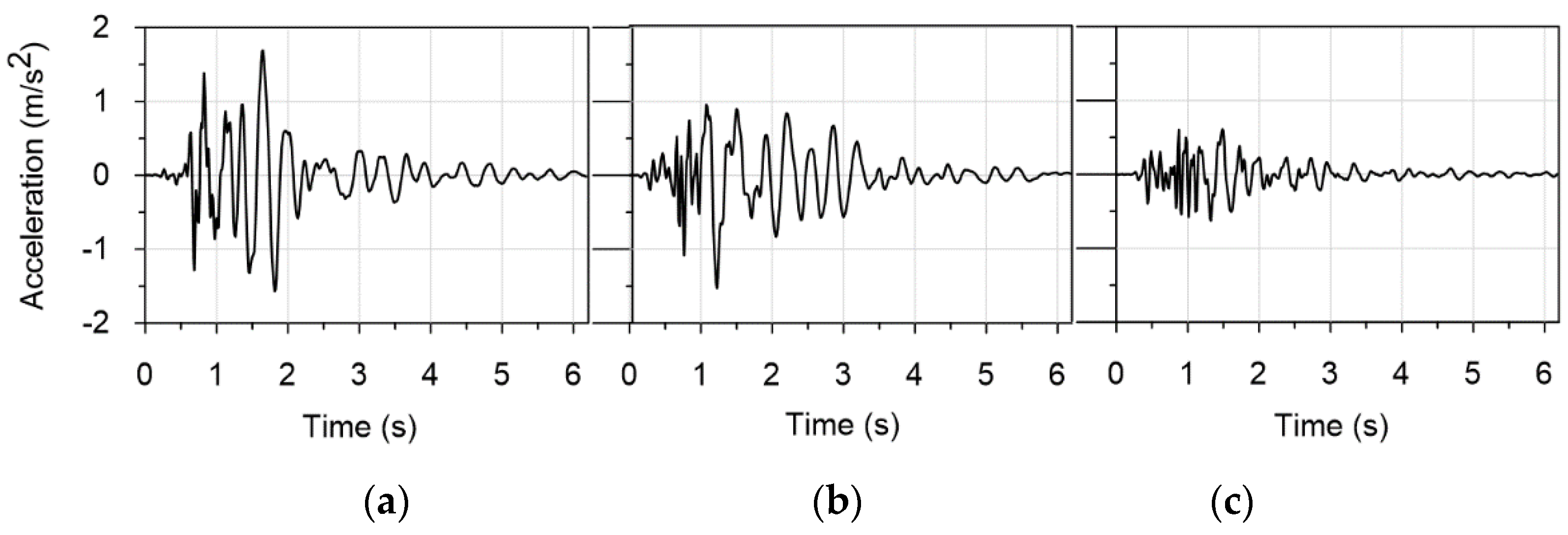
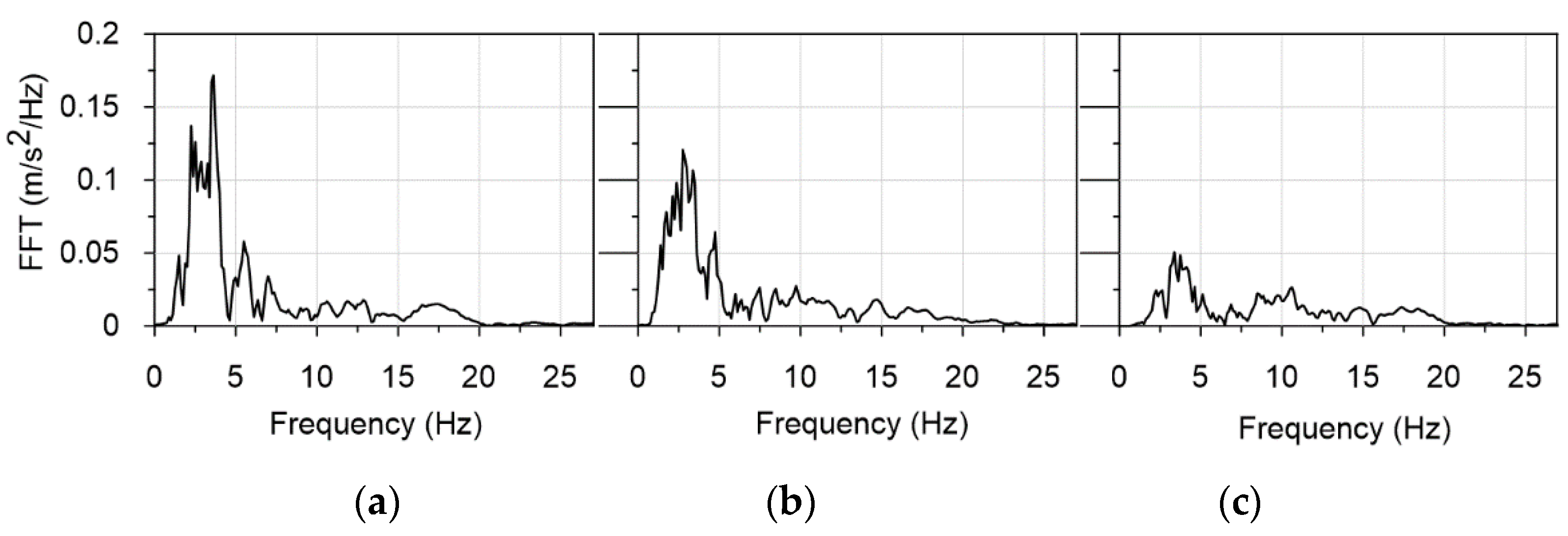
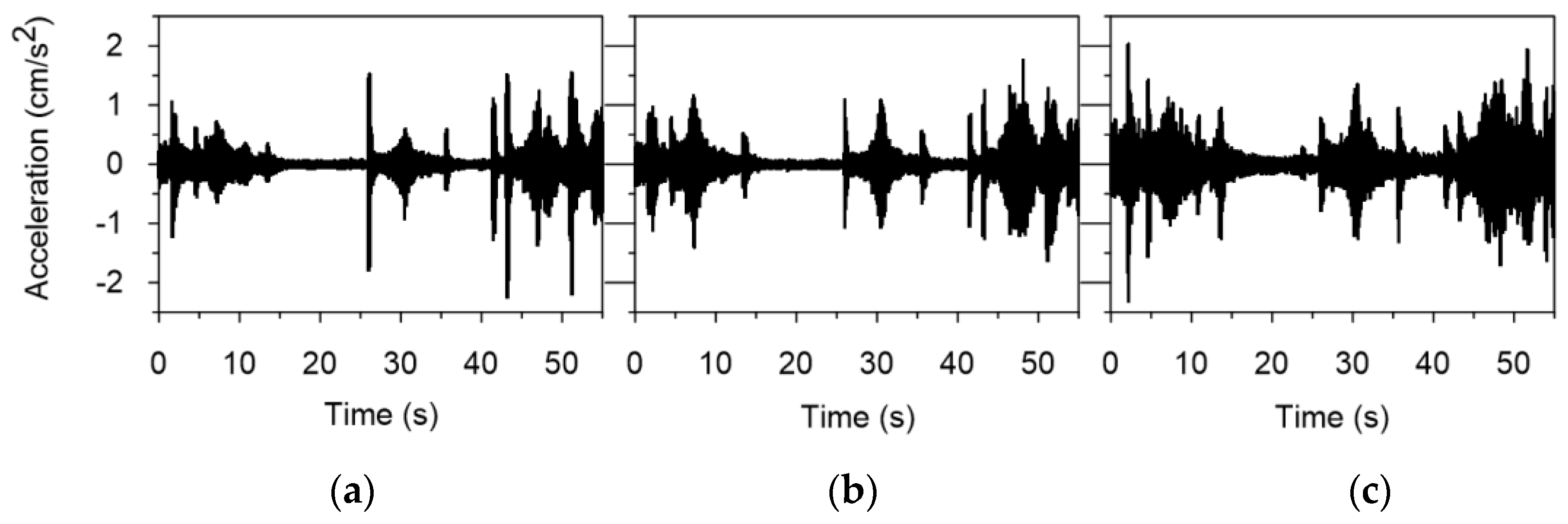
2.1. Data of the Mining-Triggered Tremor Registered in the Upper Silesian Basin, Poland
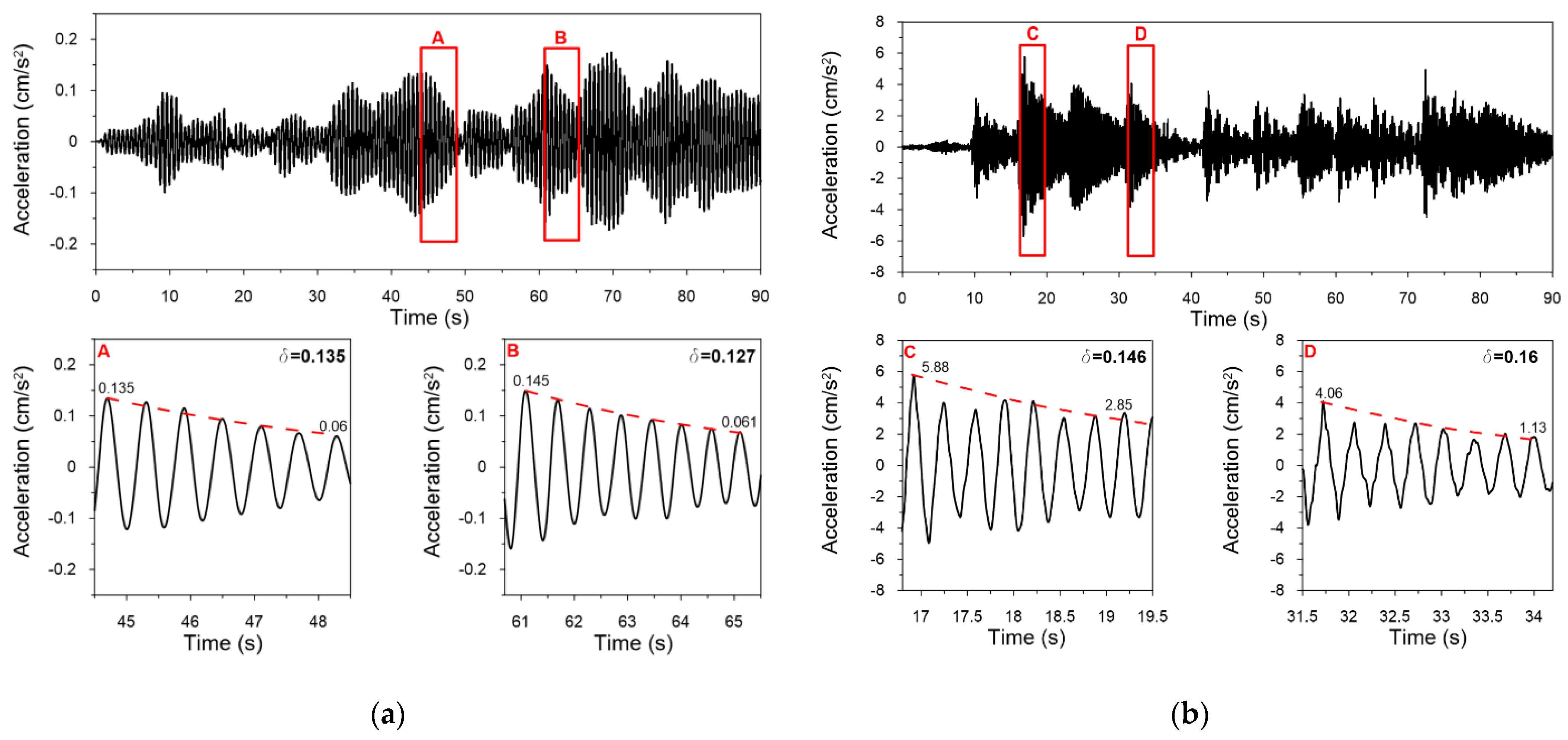
Mining-triggered seismicity has become a considerable problem in several mining activity regions in Poland. The assessment of the harmfulness of vibration for engineering structures in these regions is based on empirical scales (e.g., [35,36,37]), which enable engineers to determine the degree of vibration intensity and to estimate its influence on civil infrastructure. One of the most seismically active regions in Poland is the Upper Silesian Basin (USB), in which mining-induced seismicity hazards and the intensity of shocks have recently increased. To assess the impact of mining-induced tremors on civil infrastructure in this region, the empirical mining tremors intensity scale GSI-GZWKW-2012-A was proposed [37]. The scale refers to buildings as well as linear underground infrastructure facilities, like tunnels or water, gas, and sewage networks.
The basic parameters necessary to assess the impact of surface vibrations caused by mining tremors using the GSI-GZWKW-2012 A scale are [15]:
(a)
The maximum value of the resultant horizontal acceleration in the free field PGAH10 obtained based on filtered components of the recorded horizontal vibrations in the band up to 10 Hz (the subscript H10 means: H-horizontal accelerations, 10–maximal frequency in the filtered vibrations in (Hz)),
(b)
The duration of the intense vibration phase tHa (tHa is the time interval between moments where the Arias intensity [38] measure of horizontal acceleration reaches 5 and 95% of its maximum value).
The scale distinguishes five degrees of vibration intensity: degree “0”—no damage effects on buildings occur; degree I—sporadically increases in existing damage; degree II—enlargement of preexisting damage to nonstructural elements; degree III—first new damage on nonstructural elements occurs; and degree IV—isolated damage of structural elements occurs.
The main objective of this study is to judge the possibility of using FE models of bridges tuned and updated based on low-energy small-amplitude ambient vibrations for the calculation of the dynamic response of these structures to mining-induced tremors of different intensities. To accomplish this objective, a mining-triggered shock registered by a seismic station located in the USB region [11] was taken into consideration as a kinematic excitation of the analyzed concrete arch bridge. The duration of the intense vibration phase tHa was about 3.5 s. The energy of the shock was 1 × 10⁷ J, which puts it in the category of high-energy events. The maximum horizontal PGA of the event reached 0.35 and 0.28 m/s2 in the W–E and N–S directions, respectively. Hence, the maximum value of the resultant horizontal acceleration PGAH10 equaled 0.46 m/s2. The maximum vertical accelerations were relatively small, and they did not exceed 0.12 m/s2. The acceleration-time histories of the shock in three directions are presented in Figure 1, whereas the frequency spectra are shown in Figure 2.
The parameters PGAH10 = 0.46 m/s2 and tHa = 3.5 s classify the recorded tremor as belonging to the II degree of vibration intensity. Since, for this study purpose, mining-induced tremors of different intensities had to be considered, the originally registered acceleration-time histories were scaled down to obtain a low-energy tremor categorized as an event of the zeroth degree of intensity. Hence, the following values of PGAH10 were used for further dynamic analyses:
  • 0.1 m/s2, which corresponds to the tremor representing the zeroth degree of intensity (tremor D_0);
  • 0.46 m/s2, which refers to the second degree of vibration intensity D_II (originally recorded tremor).
The intensities of both vibrations presented against the background of the GSI-GZWKW-2012 A scale are shown in Figure 3. It must be pointed out that about 95% of tremors, which occur in the USB region, are classified as 0, I, or II degree of vibration intensity [39]. Since the scale GSI-GZWKW-2012-A does not refer to bridges or roads, the present study serves only to assess the intensity and strength of the analyzed mining-induced shocks. Neither structural nor nonstructural damages of the bridge were investigated based on the scale.

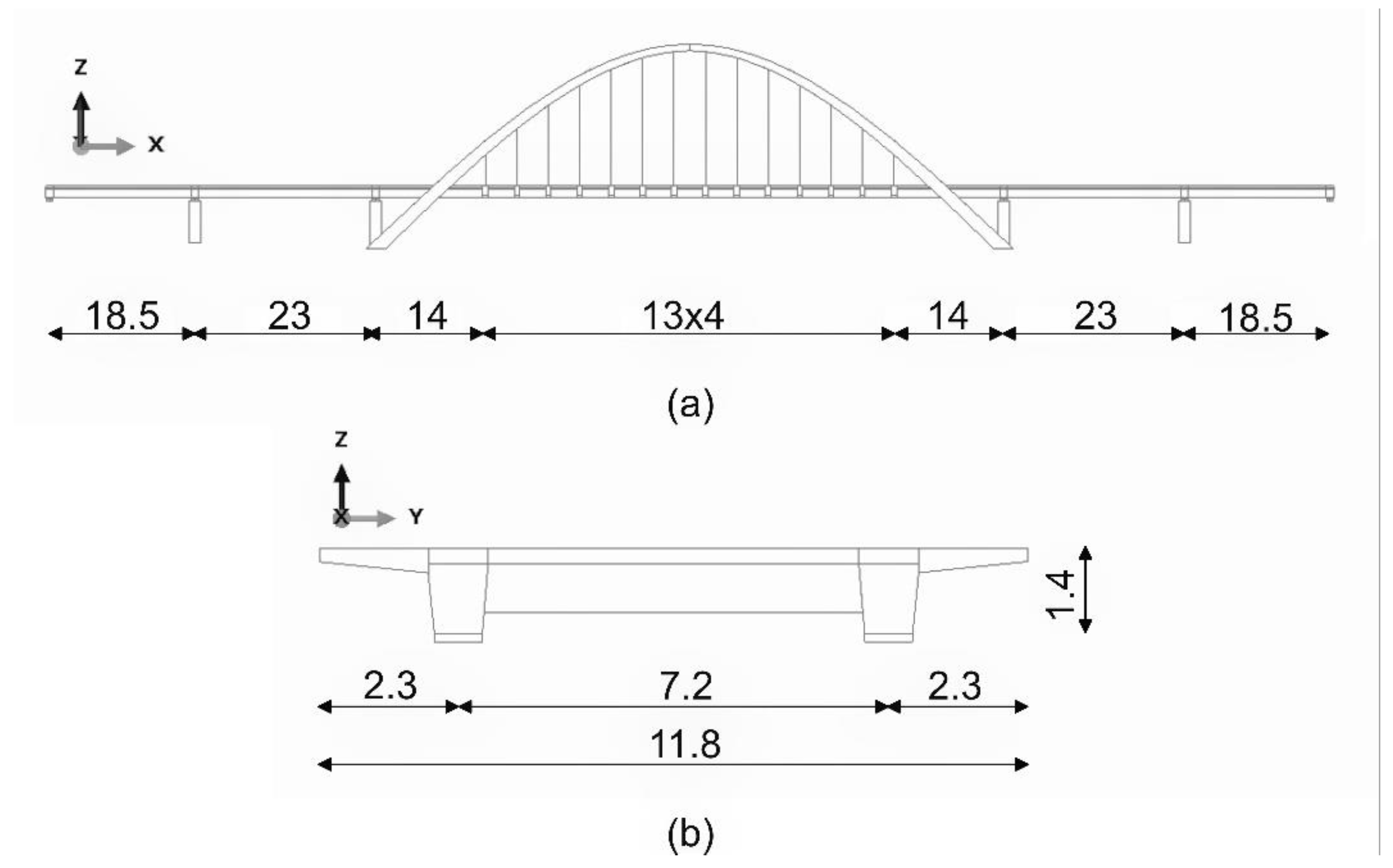
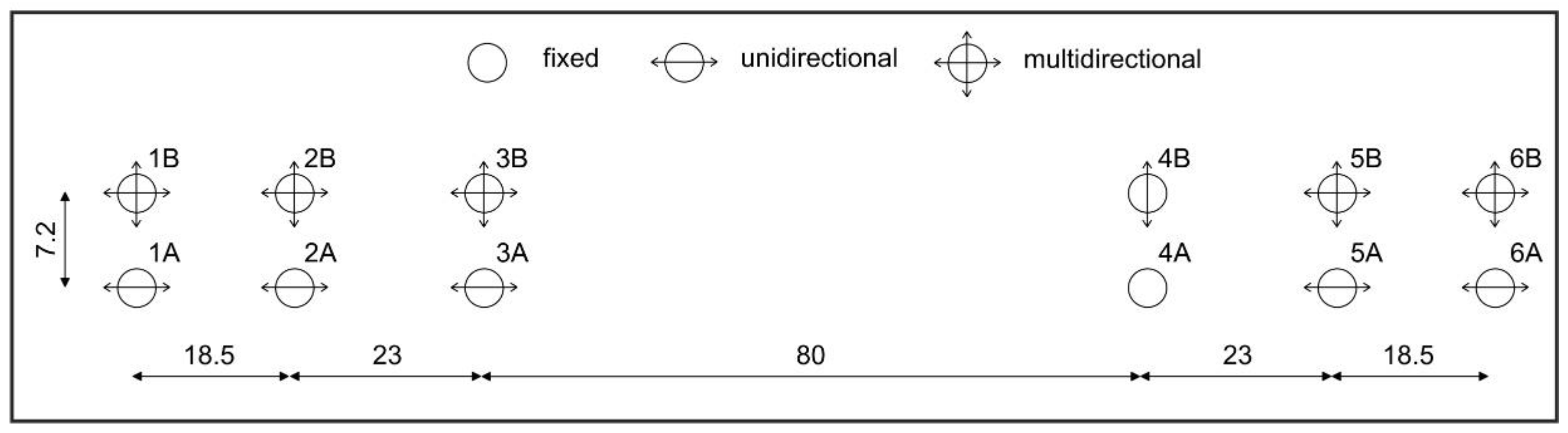
2.2. Description, Material Data and Numerical Model of the Bridge

2.2.1. Structural Layout and Material Data

The bridge analyzed in this case study (Figure 4), located in Southern Poland, was erected in 2013. The primary structural system of this five-span bridge consists of two continuous prestressed girders integrated with a concrete slab and linked by crossbars. The deck is suspended with 28 hangers on two arches over the length of the longest central span. The bridge geometry (span lengths and cross-section dimensions) is depicted in Figure 5. Each girder beam is prestressed by steel tendons with a cross-sectional area of 150 cm2. The building classes of bridge materials are collated in Table 1.
The superstructure rests on abutments and four pairs of intermediate pillars, supported by a system of pot bearings. A set of fixed and transversally guided sliding bearings is used over the supports along axis no. 4, whereas multidirectional and longitudinally guided sliding bearings are applied at other supports according to the scheme presented in Figure 6. Characteristic load-bearing capacities vary from 1500 kN (at axes 1 and 6 situated on the abutments) through 3250 kN (at axes 3 and 4) to 3600 kN (at axes 2 and 5). The pillars are 5.9 m high and have square cross-sections of 1.4 × 1.4 m.

2.2.2. The Initial FE Model of the Bridge

The numerical analysis of the bridge performance was conducted in Abaqus FEA software [40]. About 220,000 finite elements were incorporated into the model. Linear 8-node brick elements were used to discretize the girders, crossbars, arches, and pillars. The slab was meshed with 8-node continuum shell elements, whereas the hangers were modeled with truss elements (see Figure 7). Rigid structural parts like abutments or foundation footings were disregarded in the bridge model since their deformability has a negligible impact on the dynamic structure performance.
The precompression of the girders was accounted for by increasing their Young’s modulus proportionally to the steel and concrete volume fraction, according to Formula (1) [41]:
E c s = E c A c + E s A s A c + A s
where EC, AC, ES, AS are Young’s moduli and cross-sectional areas of concrete and steel, respectively.
The pot bearings were modeled by various connector element types provided by the Abaqus software: JOIN—for the fixed bearings, PLANAR for the multidirectional bearings, and AXIAL—for the unidirectional bearings. The PLANAR and AXIAL connectors allow for free translation in the direction of the predefined plane and axis, respectively.

2.3. Experimental Setup for Nondestructive Testing

Natural frequencies and modes of vibration, as well as damping ratios, were experimentally determined based on the analysis of the bridge vibration data under operating conditions. This experiment also served as validation of the numerical structure model.
During the experimental tests, acceleration-time histories were collected for the chosen structure points. The locations of these measurement points on the bridge (Figure 8a) had been determined based on numerically predicted modes of vibration. The numerical prediction was provided to fulfill the following criteria of sensors placing: (a) to avoid mounting sensors in nodes of vibration modes, (b) to place sensors at the points of maximum amplitudes appearing in the analyzed mode shapes, (c) to control the transverse mode of vibration. Hence, to accomplish the above-mentioned criteria, accelerometers were placed in the middle of the extreme span (points P1a-b), in 1/3 and 2/3 of the second span length (P3a-b, P4a-b), and in two locations of the central span: at a distance of 18.22 from the third support (P6a-b) and in the midspan (P7a-b). Additionally, sensors were located over the second (P2a-b) and third (P5a-b) supports to control the transverse mode of structure vibration. Due to the symmetry of the bridge, it was decided not to register accelerations at the other two spans. All sensors were mounted on both outer edges of the bridge deck (Figure 8b). Each measurement point was equipped with three piezoelectric accelerometers, registering data with a sensitivity of 10,000 mV/g, and a frequency range from 0.1 to 2000 Hz, in three perpendicular directions: parallel to the bridge axis (X), horizontal perpendicular to the bridge axis (Y), and vertical (Z).

2.4. Theoretical Background for the In Situ Tests

The operational modal analysis (OMA) methods [42] were implemented to identify the bridge dynamic characteristics: natural frequencies, modes of vibration, and damping properties. Experiments using OMA techniques allow for the assessment of the structure modal properties based on output response data to ambient vibrations, collected under operational conditions, without known artificial excitation. Hence, the experiment does not interfere with the normal use of the structure and is faster and cheaper than the input–output techniques. The OMA technique applied in this paper is stochastic subspace identification (SSI), one of the most applicable approaches for output-only identification methods in the time domain [43,44].
The SSI theory assumes that the registered signals are burdened with stochastic broad-band white noise. The SSI algorithm is based on the process of singular value decomposition (SVD) of the Hankle matrix, which contains experimental data. This process allows for filtering and reducing the noise and, as a consequence, leads to the identification of parameters of deterministic systems. Therefore, the raw signals (accelerations of the control points) registered in time can be used in analyses, and no signal filtering is needed [45,46,47].
The complex mode indicator functions (CMIF) are used within the SSI algorithm to determine the natural frequencies of a structure. The CMIFs are computed based on the singular value decomposition (SVD) of the normal matrix, using the cross-correlation between data sets. The peaks detected in the CMIF plot indicate the existence of modes, and these peaks’ corresponding frequencies provide the natural frequency for each mode [48,49,50]. Since an inappropriate (too large or too small) experimental data set may lead to incorrect results, the stability of the poles should be verified. Only stable poles appearing in the CMIF matrix can be treated as a structure’s modes (unstable poles are mathematical objects without physical interpretation). The pole stability control process is described in detail in [51,52]. Accuracy of the modal properties obtained with CMIF depends on the proper selection of the method parameters: the model order and convergence (stability) criteria like frequency error, damping error, and modal vector similarity. The most important parameter is the model order (the system’s number of degrees of freedom), which determines the number of modal frequencies obtained from the experimental data. Therefore, the value of the model order should be derived from the number of experimental sets and correspond to the required number of modes. Over- or underestimation of the model order leads to inaccurate values of modal parameters. The modal vector similarity specifies the minimum required degree of similarity of eigenvectors. If the modal parameters for two subsequent iterations meet all defined convergence criteria, the pole is considered stable. Otherwise, the mode is treated as an unstable pole [50,53,54,55].
To determine the structure’s mode shape for each stable pole based on the experimental data, the time domain decomposition (TDD) technique is used. In the TDD algorithm, the registered signals must be filtered using band-pass filters, with bands containing the frequencies of the single expected mode. Based on the filtered time history of acceleration, the consecutive mode shapes are determined by the SVD of the signal using the energy correlation matrix of the isolated (filtered) accelerations. Due to the rapid convergence of the TDD, this technique is especially useful for ambient modal analysis [45,56,57].
The recognition of the dynamic properties of a structure should be complemented by the evaluation of damping parameters. The level of structural damping is usually governed by the logarithmic decrement of damping (δ) and the damping ratio (ξ) [58]. The Rayleigh model of mass and stiffness proportional damping [44] was applied for the seismic analysis of the bridge. The model assumes that the damping matrix is represented by a linear combination of the mass matrix and the stiffness matrix. The proportionality coefficients are determined based on the natural frequencies and corresponding values of damping ratios [44].

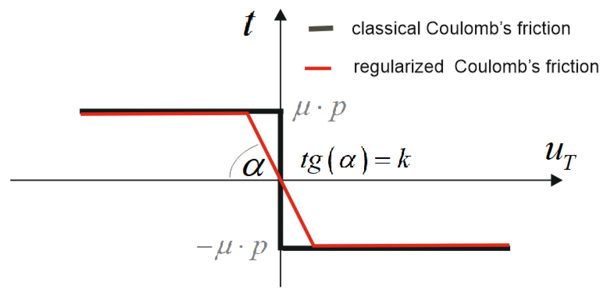
2.5. Theoretical Background for Frictional Contact Based on Elasto-Plasticity with Associated Sliding Rule

To account for the friction phenomenon occurring in sliding bearings under both operational loads and large horizontal loads, appearing, for instance, during seismic events, the frictional stick-slip model is introduced.
In the standard Coulomb friction model, the relation between the relative motion of two surfaces in contact and the frictional tangential stress takes the form:
u ˙ T = { 0   if   | t | < μ p λ t | t |   if   | t | = μ p
where: u ˙ T –vector of relative displacement rate tangent to contacting surfaces, p –normal contact stress (pressure), t –tangential contact force density (frictional tangential stress), μ –coefficient of friction, λ –negative scalar multiplier.
In this model, there is no relative motion unless the frictional stress reaches the critical value. Coulomb friction law can be alternatively formulated within the framework of elastoplasticity [59,60]. In this approach, the tangential relative displacement rate between contacting surfaces is split into the reversible elastic part u ˙ T e and the irreversible sliding u ˙ T p :
u ˙ T = u ˙ T e + u ˙ T p
The reversible relative tangential motion from the point of zero frictional stress is governed by Equation (4):
t = k u T   if   | t | < μ p
which is equivalent to the introduction of the elastic constitutive law for the tangential relative micro displacements between the contacting surfaces in the stick state. The behavior remains elastic as long as the frictional stress does not reach the slip criterion (analogy to the yield criterion):
f ( t , p ) = | t | μ p = 0
Sliding is governed by the sliding rule (analogous to the associated plastic flow rule):
u ˙ T p = λ f t = λ t | t |
The assumption of the existence of the elastic microslip preceding macrosliding is based on experiments (e.g., [61]) and can be explained by the deformation of asperities (roughness of contacting surfaces on the microscopic scale).
This formulation can also be seen as the regularization of the stick-slip behavior, allowing to avoid the numerical difficulties due to the non-differentiability of the classical Coulomb’s law at the onset of sliding [62] (see Figure 9).

3. Results

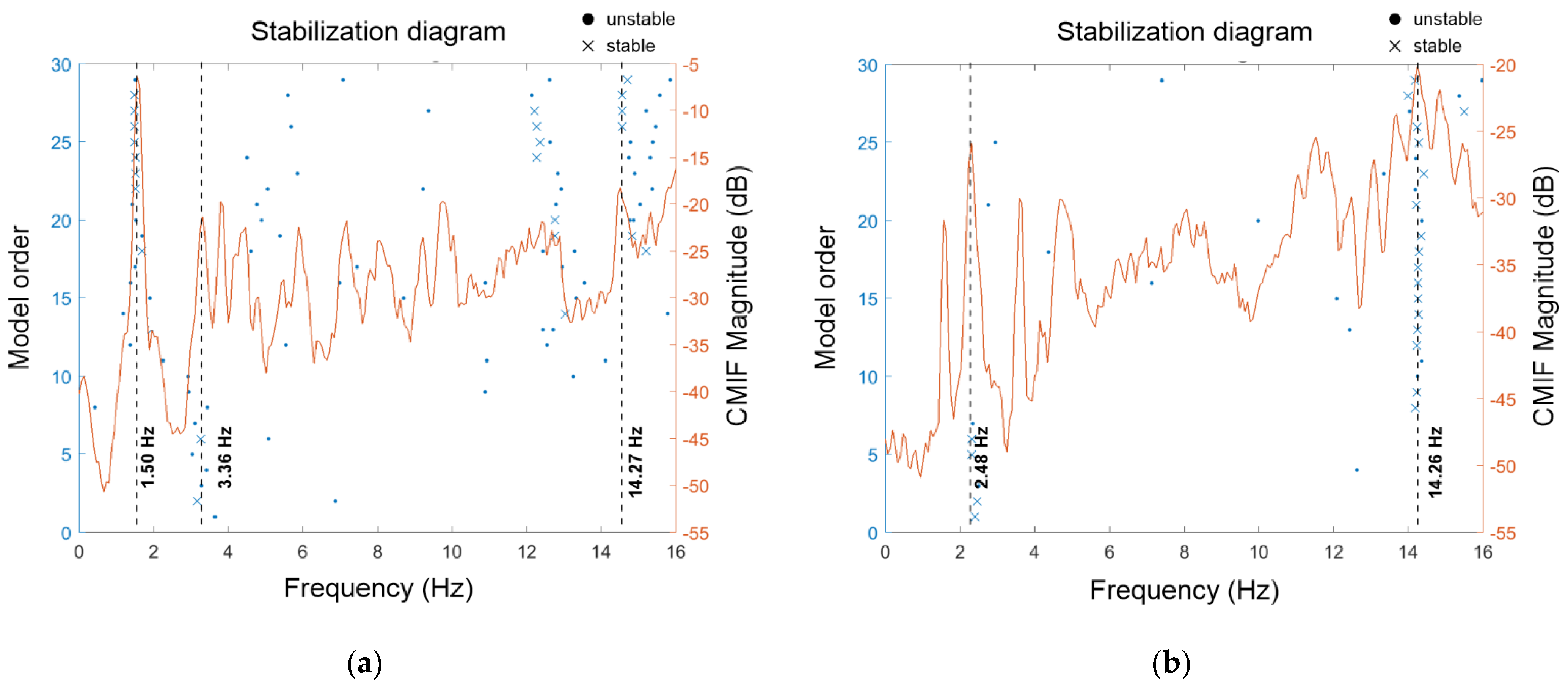
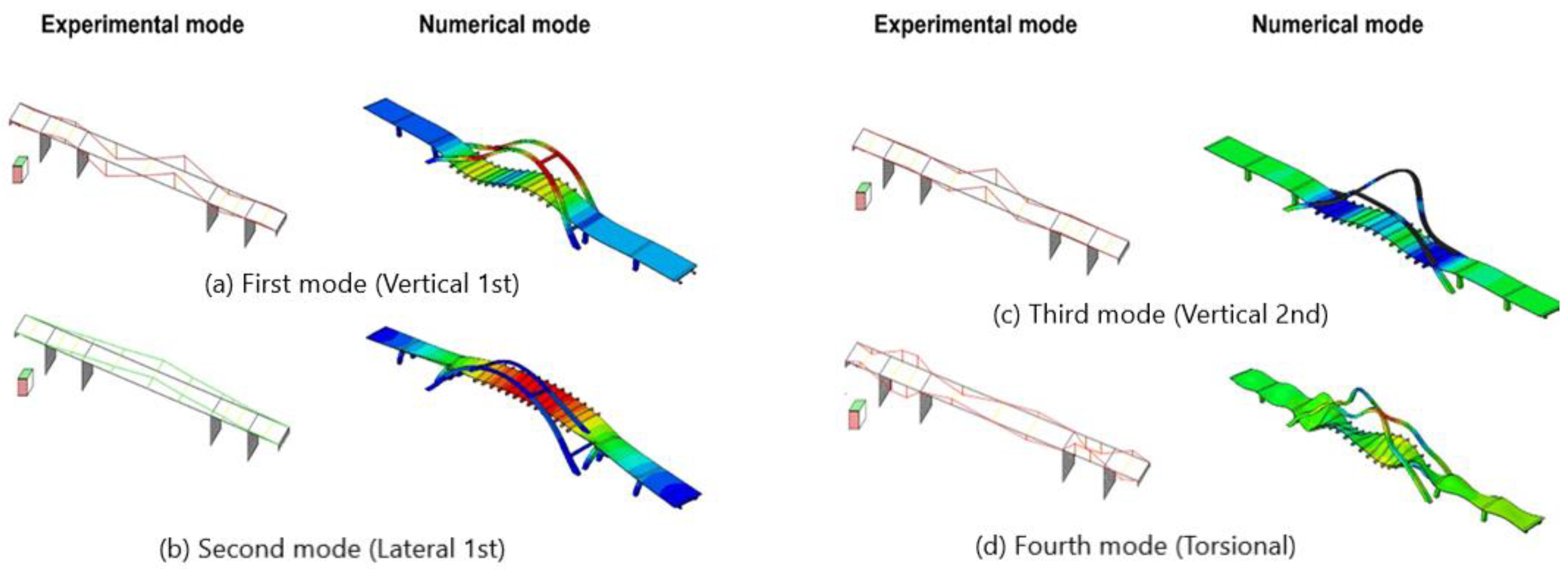
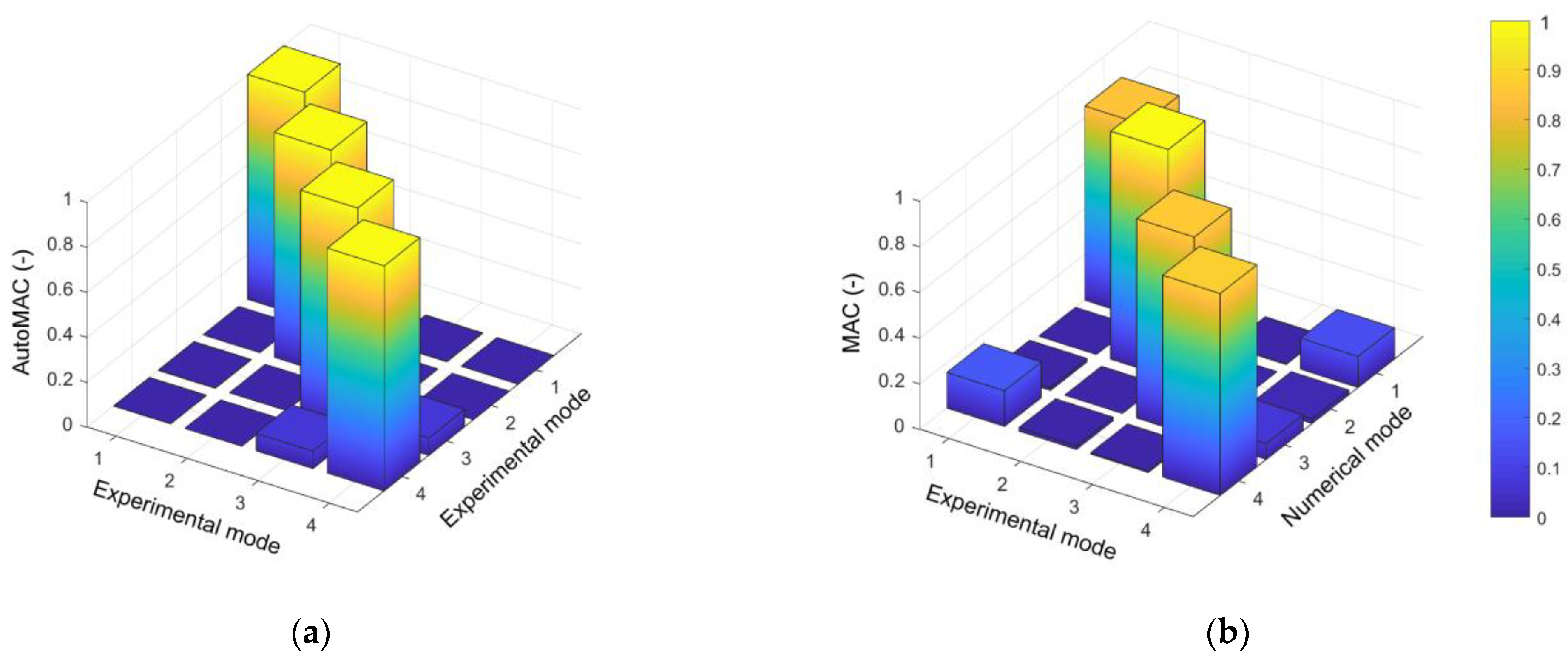
3.1. Experimental and Numerical Evaluation of Natural Frequencies and Modes of Vibration of the Bridge

In the first stage of the research, the natural frequencies and modes of vibration of the bridge were experimentally and numerically determined and compared.
First, the preliminary modal analysis of the FEM model was carried out, and the basic natural frequencies and mode shapes were estimated. The following natural frequencies were recognized numerically: f1 = 1.57 Hz–(corresponding to the first vertical mode shape) f2 = 1.87 Hz (associated with the first transverse mode shape), f3 = 3.48 Hz–(related to the second vertical mode shape), and f4 = 14.30 Hz (associated with the first torsional mode shape). The preliminary numerical modal analysis also revealed that, due to the complexity of the structural system of the bridge, mode shapes corresponding to frequencies located above the limit of 15 Hz were much more complicated, affecting mainly the arches and hangers. Hence, both the experimental and numerical modal analyses covered only the frequency range from 0 to 15 Hz, where the basic four natural frequencies related to vertical, horizontal, and torsional modes are placed. Higher frequencies were not identified in the research.
Second, the experimental modal analysis of the bridge was conducted using the OMA techniques and the SSI algorithm to estimate natural frequencies and the TDD method to determine modes of vibration corresponding to the estimated frequencies (see Section 2.4). The acceleration-time histories resulting from ambient vibrations, i.e., wind and road traffic, were registered at all output points. The 55 s fragment of acceleration-time histories registered at point P7a in three directions as a result of ambient vibration is presented in Figure 10. The CMIF natural frequency estimator of the experimental modal model (see Section 2.4), based on the summation of all combinations of PSD and CSD functions between data recorded at all output measurement points, is illustrated in Figure 11 for the vertical and horizontal directions. The following parameters of the CMIF estimator were applied in the analysis: order–30; convergence–90%; frequency and damping error–2%.
It can be observed from Figure 11a that the peaks and the stable poles of the CMIF diagram in the vertical direction are located at frequencies 1.50, 3.36, and 14.26 Hz. Additional stable poles, appearing around 12 Hz, are not confirmed as the maximum values of the CMIF magnitude or in the numerical prediction. For the horizontal direction, the maximum values and the stable poles are observed in Figure 11b at the frequencies 2.48 and 14.26 Hz.
Finally, the results of the experimental and numerical analyses were compared. The first four natural frequencies obtained experimentally and numerically are collected in Table 2, whereas the corresponding modes of vibration are presented in Figure 12.
The comparison of experimentally and numerically obtained natural frequencies indicates a high level of consistency between the values calculated based on both methods for the first, third, and fourth frequencies, where the discrepancies do not exceed 5%. For such a level of structural system complexity, the similarity between numerical and experimental results can be considered satisfactory if the differences are lower than 7% [63]. The only exception appears in the case of the second natural frequency corresponding to the transverse mode shape (see Figure 12b), for which this discrepancy is much greater, reaching almost 25%, far above the acceptable limit. Hence, the goal of the first step of the FE model tuning strategy was matching the numerical transverse mode frequency with the measured value to meet the modal identification requirements. It is also worth mentioning that all experimental and numerical mode shapes show very high compliance.

3.2. Experimental Evaluation of Damping Properties

In the research, the values of logarithmic decrements of damping were determined for the frequencies corresponding to the first and the second vertical mode shapes. The estimation was based on discrete experimental data acquired during the jumping test, in which four people jumped vertically synchronized by a metronome. The registered acceleration-time histories were filtered by the 3rd order digital Butterworth filter with the bandwidth 0.04 Hz, centered at the estimated natural frequencies.
Exemplary free decay plots for the frequency related to the first and second vertical vibration modes are shown in Figure 13a,b, respectively. Such plots, obtained for all measurement points, were the basis of the evaluation of the logarithmic damping decrements and damping rations.
The average values estimated for the logarithmic decrements were δ1 = 0.13 and δ2 = 0.17 for the first and second vertical modes of vibration, respectively, leading accordingly to the damping ratios ξ1 = 2.1% and ξ2 = 2.7%.
On the basis of the obtained damping ratios, the coefficients of Rayleigh’s damping model were estimated as α = 0.21 and β = 0.00208 and applied in the seismic analysis of the bridge.

3.3. First Step of the Tuning Strategy: Calibration of the FE Model Based on the Experimental Modal Identification

Prior to the presented tuning strategy involving sliding bearings, two other variables were taken into account in the process of manual tuning: (a) Young’s modulus of the pillars and (b) Young’s modulus of the deck. The first tuning attempt consisted of increasing the structural rigidity in the transverse direction by a modification of the pillars’ Young’s modulus to account for the maximal allowable reinforcement percentage (4%) according to Equation (1). This approach was abandoned since it resulted in an insufficient growth of the second natural frequency to 1.9 Hz (still 17% below the experimental value), simultaneously increasing the first frequency to 1.6 Hz and thus worsening its compliance with the experiment. Increasing Young’s modulus of the deck also resulted in significant growth of vertical frequencies.
Other possible sources of the FE model inadequacy are damages or failures of bridge structural elements. Periodic bridge inspections in Poland are regulated by a document issued by General Directorate for National Roads and Motorways [64], defining two types of inspections: (a) yearly basic inspection checking for possible damage and inspecting the condition of installation and equipment and (b) detailed inspection performed every 5 years, examining the technical and functional state of all structural elements. The condition of every structural element is assessed on a 6-point rating scale, where 5 means “without any damage” and 0 means “failure”. The analyzed bridge underwent a detailed inspection in 2018 [65] (the year in which the authors carried out the experiment). All structural bridge elements were assessed for 5 in the above-described scale. The yearly inspection in 2020 [66] confirmed these results. Hence, the decision was made to neglect the influence of any possible damage of structural elements on the bridge dynamic behavior.
Taking into consideration the above-mentioned explanation, the authors decided to focus on sliding bearing modeling as a potential source of the inadequacy of the FE model frequency corresponding to the lateral mode shape.
In the primary numerical model, the sliding between bearing surfaces was assumed as a frictionless connection. Such simplification does not reflect the real behavior of a sliding pot bearing. The neglect of friction forces in the sliding bearings resulted in the lack of cooperation between the pillars and the slab under horizontal motion, leading to the underestimation of the structure’s transverse stiffness.
It has been reported in the literature and proven experimentally [27] that during low-energy ambient vibration bridge testing, horizontal excitations are small, generating forces in the bearings below the sliding limit. Authors suggest that for the modal analysis, one should assume that all bearings are fixed (without the possibility of sliding in any direction). In our case, this assumption provided a satisfactory correction of the second (horizontal) natural frequency (with discrepancies below 2%), but at the same time, it spoiled the adjustment of the first (vertical) frequency, which jumped to 1.90 Hz, 27.5% over the experimental value.
To avoid excessive stiffening of the model at the bearings, its calibration in the present study has been conducted by attaching horizontal linear springs to the sliding bearings. Since the modal analysis requires a full model linearization, applying the nonlinear frictional model (see Section 2.5) to represent the bearing behavior was not an option at this analysis stage. However, the stick part of this model is equivalent to adding horizontal springs with constant stiffness Ks (see Figure 14) to the connectors representing sliding bearings to account for the frictional interaction.
To roughly estimate the spring stiffness, two simplified one-dimensional models of the bridge were analyzed as single-degree-of-freedom (SDOF) frames oscillating in the transverse direction. In these models, the deformation of the deck is ignored, the rigid deck vibrates on the bending columns (Figure 15).
The frame with sliding support at the right pin beam–column connection (see Figure 15a) represents the unrefined FEM bridge model with frictionless sliding at bearings. The natural frequency of this frame (or its equivalent mass–spring representation) takes the form:
f a = 1 2 π K c m
where: m is the oscillating mass and K c = 3 E I h 3 is the bending stiffness of the left frame column, treated as a cantilever beam, with h ,   I ,   E meaning column height, cross-sectional inertia moment, and material’s Young’s modulus, respectively.
The frame with a frictional elastic stick at the right pin beam–column connection (see Figure 15b) represents the updated FEM, in which the right column is involved in the frame vibrations via the elastic spring representing the elastic stick friction in the bearing. The equivalent stiffness of the system of two pillars (with bending stiffness KC each) and the spring representing elastic stick with coefficient KS can be determined as:
K = K c + K c K s K c + K s = K c K c + 2 K s K c + K s
It leads to the natural frequency of this SDOF system:
f b = 1 2 π K m = 1 2 π K c m K c + 2 K s K c + K s
After designating the ratio of the natural frequencies of both frames as:
α = f b f a = K c + 2 K s K c + K s
one can determine the dependence of the stiffness of the elastic stick spring on the bending column stiffness K c and the frames’ frequency ratio α:
K s = K c α 2 1 2 α 2
This formula can serve as a rough approximation of the elastic stick coefficient, which should be used in the bridge bearing friction model to fit the numerical first transverse natural frequency to the experimental value.
The bending stiffness of the analyzed bridge pillars equals KC = 147 MN/m, the transverse frequency of the primary FE model is fa = 1.87 Hz, and the desired transverse frequency of the updated FE model should be equal to the experimental value fb = 2.48 Hz (see Table 2). Substituting the above values into Equation (11) gives the approximation of the elastic stick coefficient equal to KS = 462 MN/m.
The value of the elastic stick coefficient, which leads to the best compatibility between experimental and numerical values of all four analyzed frequencies (based on the least square method), equals KS = 400 MN/m. This value was used in the stick part of the frictional contact model (see Section 2.5) in the seismic analysis of the bridge. Raising the spring stiffness above this value led to an excessive increase of the first vertical frequency.
The comparison of natural frequencies calculated using the calibrated FEM model with the experimental values is presented in Table 3. One can notice much better compliance of the results than for the primary model for the horizontal modes. The spring connection, which guarantees the cooperation between the slab and both pillars during horizontal vibration, leads to the increase in the transverse stiffness of the structure. As a consequence, the value of the second natural frequency also rises. The discrepancies between the experimental and numerical (for the modified model) frequencies do not exceed 8% in any case. Such a result seems to be satisfactory, taking into consideration the complexity of the structure. It is also worth mentioning that there are no significant changes in the numerical mode shapes.
Authors of similar studies devoted to experimental and numerical investigations of the dynamic properties of bridges with comparably complex structures indicate a similar level of compliance between measured and calculated eigenvalues. For example, in the analyzed cases of a prestressed composite box-girder bridge [63], an arch railway bridge [67], and a long-span cable-stayed bridge with a steel box girder [68], the maximal discrepancies between the natural frequencies identified experimentally and derived numerically reached 6.8, 7.5, and 6%, respectively.
To confirm the correctness of the mode shape vectors, verification with the modal assurance criterion (MAC) was performed [69]. The MAC procedure allows for the quantitative comparison of mode shapes obtained from different methods to avoid mistakes (i.e., duplication of modes). Based on this method, one can determine the similarity of two modes by evaluating MAC parameters with the following formula:
M A C i j = ( φ A i T φ B j ) 2 ( φ A i T φ A i ) ( φ B j T φ B j )
where φ A and φ B are the modal vectors obtained with methods A and B, respectively. The M A C   parameters can take values ranging from 0 (meaning no correspondence between modes) to 1 (representing a full correspondence).
First, the AutoMAC matrix was determined, comparing the experimentally identified mode shapes (Figure 16a). The results prove that particular modes differ from each other and do not duplicate. Then, the experimentally and numerically determined modes were compared using the MAC procedure (Figure 16b). It may be noted that the values located on the MAC matrix main diagonal are higher than 0.8, which indicates the consistent correspondence between the appropriate modes (modes with the same numbers) from the experiment and numerical analysis. The off-diagonal MAC matrix elements do not exceed 0.2, proving the correct matching of the modes obtained by both methods.

3.4. Second Step of the Tuning Strategy: Modification of the FE Model for Mining-Induced Seismic Performance Assessment

Updating the FEM model by attaching springs to the connectors representing sliding bearings allowed to closely match the experimentally measured natural frequencies. This model can perform well under operational loads when the assumption of the absence of sliding at bridge bearings can be justified. However, under heavy excitations generating significant horizontal forces, the bearing plates slide relative to each other. The frictional force produced in the sliding pot bearing is bonded by the coefficient of friction between the sliding surfaces of the bearing piston, usually covered by polytetrafluorethylene (PTFE), and the soleplate, made of stainless steel. The design friction coefficient in pot bearings ranges from 0.03 to 0.06 [70]. Since the linear spring attached to the connector modeling the bearing parts produces a force proportional to the relative motion, it cannot represent sliding.
To account for the proper modeling of bearing behavior under different loadings, the second update of the bearing model was introduced. The frictional contact based on elastoplasticity with the associated sliding rule (see Section 2.5) was adopted as the constitutive model for bearing connectors. The elastic constant k, representing the stick stage (Equation (4)), was taken as the linear spring stiffness KS determined in the first stage of model tuning. The friction coefficient in the slip criterion (Equation (5)) was assumed as 0.04, which is in the range of design friction coefficients of pot bearings.

4. Discussion

4.1. Comparative Analysis of Dynamic Performance of the Bridge under Mining-Induced Shocks of Various Intensity: Untuned vs. Tuned FE Models

4.1.1. The General Framework of the Comparative Analyses

The dynamic performance of the bridge was assessed for two mining-triggered shocks of various intensities: D_0 with PGAH10 = 0.1 m/s2 and D_II with PGAH10 = 0.46 m/s2 (see Section 2.1). The time history analysis (THA) algorithm [71], based on the direct integration of equations of motion at each time increment, was implemented to calculate the dynamic responses of the bridge to the shocks. Due to its high accuracy, the THA method is suggested in EC standards [72] for both linear and nonlinear dynamic analyses. For the THA algorithm, kinematic excitation was defined by the vector of the supports’ accelerations (see Figure 1) applied to all supports.
The calculations were conducted with the Hilber–Hughes–Taylor time integration algorithm provided in the ABAQUS software for a direct step-by-step solution [40].
The dynamic responses (in terms of maximum principal stresses) were calculated for selected representative elements of the structure. The elements were situated on the girders above the supports and in the middle of the longest span (see Figure 17). Accordingly to the bearing specification (see Figure 6), elements 2A, 3A, 4A, and 5A were placed over fixed or longitudinally guided sliding bearings, whereas elements 2B, 3B, 4B and 5B were positioned above the transversely guided sliding bearings. Elements S1 and S2 were located in the middle of the main span.
Three FE bridge models were used for the dynamic performance assessment of the structure under the mining-induced shocks:
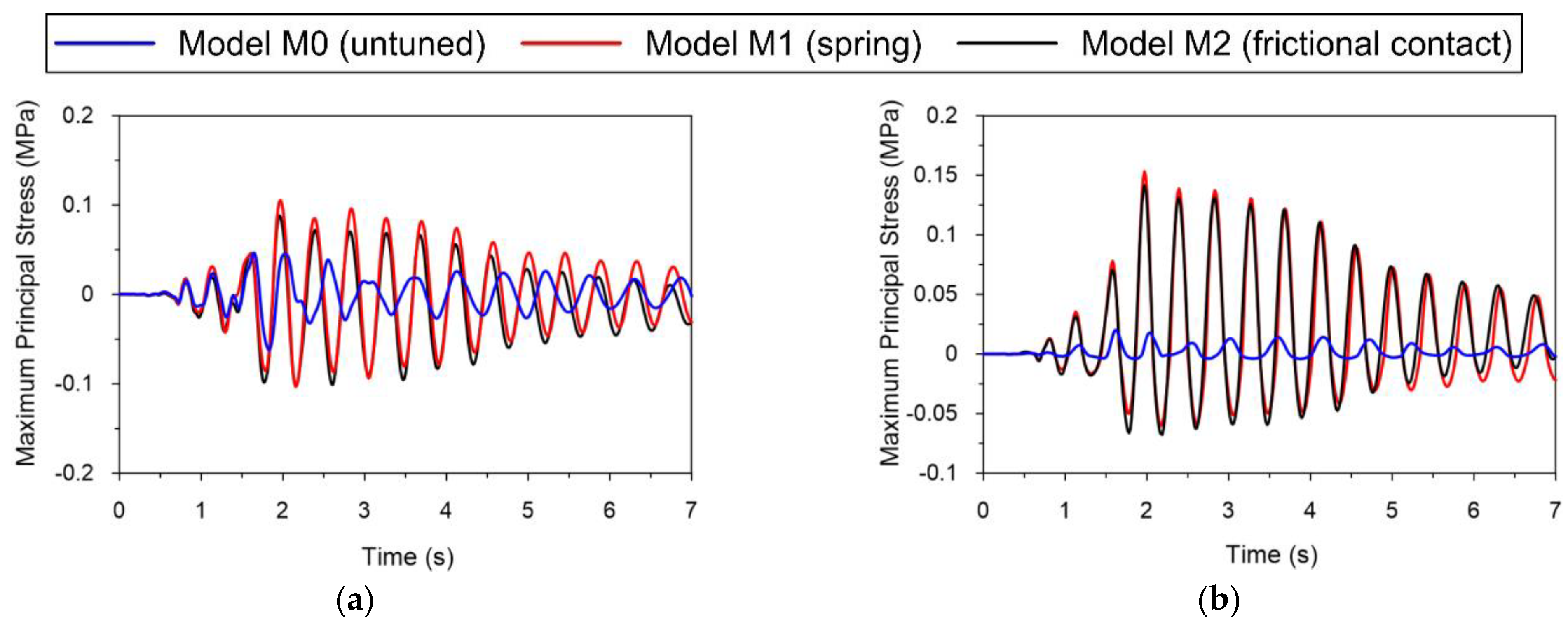
  • M0—the untuned FE model, in which the sliding between bearing surfaces was assumed as a frictionless connection (see Section 2.2.2);
  • M1—the “half” tuned FE model, after the first step of the tuning strategy, with the horizontal linear springs attached to the sliding bearings (see Section 3.3);
  • M2—the fully tuned FE model, after the second step of the tuning strategy, with frictional regularized contact, applied as the constitutive model for bearing connectors (see Section 2.5 and Section 3.4).
Considering the results gathered for all representative elements, it was decided to present a graphical comparison of the maximum principal stresses obtained for the three above-mentioned FE bridge models in elements S1 and B3.

4.1.2. Dynamic Performance of the Bridge under the Tremor of the Zeroth Degree of Intensity (D_0)

The dynamic responses of the bridge to the low-intensity tremor (D_0), obtained with models M0, M1, and M2, are summarized in Figure 18. The comparison for element S1, located in the middle of the longest span (see Figure 18a), clearly shows that the principal stresses obtained for models M1 (“half” tuned-with springs) and M2 (fully tuned-with frictional contact) are almost identical. In contrast, the stresses obtained for model M0 (untuned, with ideally sliding bearings) are approximately twice smaller. The comparison for element 3B, located above the sliding bearing, presents an analogous tendency (see Figure 18b). However, the stresses obtained for model M0 account for only 10% of the stresses received for models M1 and M2. Similar relations are observed for other elements located over sliding bearings (2B, 4B, 5B).
The forces generated in bearing (connector) 3B for models M1 and M2 are almost identical (Figure 19a) for tremor D_0. The slight difference in the time–force histories can be explained by the fact that in the M2 model at about 1.6 s of the shock, the friction-to- normal contact force ratio on the surface of the bearing reached the highest possible value of 0.04, equal to the assumed friction coefficient (Figure 19b). Thus, the stick between both bearing surfaces is broken. They slip, releasing energy, and then establish a new stick position after the change of the tremor direction.
The seismic responses observed for elements S1 and 3B can easily be explained. The spring/friction connections implemented in the bearings in models M1 and M2 established the cooperation between the girder and the pillars located beneath the sliders. This resulted in: (i) an increase of the stress level in the middle of the main span (point S1 located far from the bearings), and (ii) a significant increase of the local stresses in the girder (point 3B placed over the transversely guided sliding bearings).
It is also worth noticing that the time history response for the M0 model has a lower frequency than that for the M1 and M2 models. This results from the fact that the second natural frequency is lower in the untuned M0 model (1.87 Hz) than in the tuned M1 and M2 models (2.3 Hz). This discrepancy is substantial enough to produce the dissimilar amplification of the dynamic responses of the structure. The transverse natural frequencies of both tuned models are close to the predominant tremor frequency range in the horizontal direction (2.4–5.0 Hz, see Section 2.1). Thus, due to the resonance phenomenon, the stress amplitudes are considerably larger than in the case of the untuned model.
The presented analysis proves that the proposed fully tuned model M2 behaves similarly to model M1 (with springs adjusted based on the experimental modal identification). Both models are suitable for assessing the dynamic bridge performance under low-intensity tremors, which predominantly do not activate sliding at bearings. The opposite conclusion can be drawn for the untuned model M0. The assumption of frictionless contact enforces sliding in bearings under arbitrarily small horizontal excitations, which is unrealistic. Hence, the untuned model is not suitable for dynamic bridge assessment in the case of low-intensity tremors. The stresses obtained for this model turned out to be strongly underestimated.

4.1.3. Dynamic Performance of the Bridge under the Tremor of the Second Degree of Intensity (D_II)

The dynamic responses of all analyzed bridge models to the stronger tremor (D_II) are summarized in Figure 20. The proportions between the responses of “untuned” M0 and “half-tuned” M1 models are the same as in the case of the D_0 tremor (Figure 18), namely: the stress amplitudes acquired with the M1 model are approximately twice greater at point S1 and ten times greater at point 3B, than these obtained with the M0 model. This result is obvious since, due to both models’ linearity, the responses are proportional to applied loads. However, a meaningfully dissimilar dynamic performance under the stronger tremor is observed for the “fully tuned” model M2, which, due to the frictional contact formulation, is nonlinear. In this case, the stresses in the representative element located far from the bearings (S1) exhibit a strong resemblance to those obtained with the untuned model M0 (see Figure 20a), while at points located directly over the bearing (element 3B), the stress amplitudes are about twice bigger than those found for the untuned model M0, but significantly smaller than values achieved with the spring equipped model M1. It should be emphasized that such significant differences in stress values are of local scope and involved only the girders’ zones located closely to the bearings. Other analyzed elements placed far from the bearings were not affected by such significant alterations in stresses.
The forces generated in the bearing (connector) 3B for models M1 and M2, as well as the friction-to-normal contact force ratio for the D_II tremor, are presented in Figure 21a,b, respectively. During each cycle of the intensive phase of the tremor, horizontal excitation in the M2 model is strong enough to induce sliding in the bearing (see Figure 21b), which results in the limitation of the frictional force in the connector to 0.04 of the normal contact force, while the force in the M1 model spring, which is not limited, is considerably greater (see Figure 21a).
Based on the presented comparisons, some conclusions can be drawn regarding the stresses obtained using analyzed models under the second degree of intensity tremor (D_II). The cooperation between the girder and the pillars beneath the sliders, introduced by the spring and friction in models M1 and M2, respectively, causes an increase in the stresses compared to those obtained with model M0. However, in the case of model M2, the spring linear force/displacement relation is replaced by the frictional contact once the sliding occurs at the bearings. This induces a rapid decrease in the stresses at both representative elements.
The presented analysis shows that only the fully tuned model M2 allows for the accurate representation of the sliding bearing performance under a high-intensity mining-induced tremor. Springs applied in the M1 model generate unrealistically large horizontal forces in bearings, resulting in a considerable overestimation of the structural dynamic response (especially for vibrations with dominant frequencies close to the transverse bridge natural frequency). On the other hand, the frictionless sliding in the M0 model leads to the undervaluing of the local structure response, although the global stress level is estimated correctly. Additionally, one should bear in mind that this model underestimates the structure transverse natural frequency. For the above reasons, neither the “half tuned” M1 model nor the untuned M0 model is applicable for assessing the dynamic performance of the bridge under high-energy mining-induced shocks.
It must be pointed out that similar assessments of the dynamic performance of the bridge were performed for other degrees of tremors’ intensity: D_I, D_III, D_IV (see Figure 3). In all cases, the results turned out to be analogous to these obtained for the tremor D_II.

5. Conclusions

In this paper, a two-step tuning strategy of FE models of bridges with sliding bearings exposed to mining-triggered tremors is proposed, based on the numerical and experimental analysis of a bridge equipped with standard pot bearings and not fitted with a structural vibration monitoring system. The following conclusions can be drawn based on the conducted experiments and numerical calculations:
  • The comparison of experimentally and numerically obtained natural frequencies indicated a poor level of consistency between the values of the second natural frequency corresponding to the transverse mode shape. The reason for such a discrepancy lies in the primary, untuned numerical model, with assumed frictionless sliding in bearings. Such simplification is not appropriate since, due to the low level of ambient vibration, sliding in the pot bearings was prevented by frictional forces;
  • The proposed two-step tuning strategy of the FE bridge model significantly improved the consistency of the experimental and numerical values of the second natural frequency. In the proposed approach, the free bearing sliding was replaced with the Coulomb friction-regularized model, based on elastoplasticity with the associated sliding rule;
  • The comparative analysis of the dynamic responses of the bridge models to mining-triggered tremors of various intensities (from 0 to IV degree) proved that the untuned model is not suitable for structure dynamic assessment in the case of low-energy tremors (0 degrees of intensity). The stresses obtained for this model turned out to be strongly underestimated. For shocks of higher intensity, frictionless sliding at bearings gave a relatively good global estimation of structure performance but undervalued its local response. On the other hand, the model tuned with linear springs proved to be applicable only for low-intensity tremors. In case of stronger shocks (from I to IV degree of intensity), the springs applied in bearings generated unrealistically large horizontal forces, resulting in a considerable overestimation of the structural dynamic response;
  • The analysis revealed that only the fully tuned Coulomb friction-regularized model allows for the accurate simulation of sliding bearings under both low-energy and high-energy mining-induced tremors. However, it must be pointed out that this tuning strategy is valid for a particular type of bridge only, i.e., for those who benefitted from pot bearings (fixed and sliding).
It should be emphasized that due to the rapid industrial growth involving an increase in the exploitation of natural resources, an urgent need arises to protect existing road infrastructure. In that context, the proposed two-step tuning strategy may help the accurate assessment of the dynamic performance of older bridges located in mining-triggered seismic zones, not retrofitted with modern anti-seismic bearings but equipped with standard systems of fixed and sliding bearings.

Author Contributions

Conceptualization, J.M.D. and D.J.; data curation, P.B.; formal analysis, J.M.D., D.J. and P.B.; investigation, J.M.D. and P.B.; methodology, J.M.D.; supervision, J.M.D. and D.J.; visualization, P.B.; writing—original draft, J.M.D., D.J. and P.B.; writing—review and editing, D.J. All authors have read and agreed to the published version of the manuscript.

Funding

This research received no external funding.

Institutional Review Board Statement

Not applicable.

Informed Consent Statement

Not applicable.

Acknowledgments

This research was supported in part by PL-Grid Infrastructure.

Conflicts of Interest

The authors declare no conflict of interest.

References

  1. Gunning, A.P.; Lasocki, S.; Capuano, P. Assessing environmental footprints induced by geo-energy exploitation: The shale gas case. Acta Geophys. 2019, 67, 279–290. [Google Scholar] [CrossRef]
  2. Foulger, G.; Wilson, M.; Gluyas, J.; Julian, B.; Davies, R. Global review of human-induced earthquakes. Earth Sci. Rev. 2018, 178, 438–514. [Google Scholar] [CrossRef] [Green Version]
  3. Peng, P.; Jiang, Y.; Wang, L.; He, Z.; Tu, S. A Fast ray-tracing method for locating mining-induced seismicity by considering underground voids. Appl. Sci. 2020, 10, 6763. [Google Scholar] [CrossRef]
  4. Huang, Q.; Wang, X.; Chen, X.; Qin, D.; Chang, Z. Evolution of interior and exterior bearing structures of the deep-soft-rock roadway: From theory to field test in the Pingdingshan Mining Area. Energies 2020, 13, 4357. [Google Scholar] [CrossRef]
  5. Vižintin, G.; Kocjančič, M.; Vulić, M. Study of coal burst source locations in the Velenje Colliery. Energies 2016, 9, 507. [Google Scholar] [CrossRef] [Green Version]
  6. Tatara, T. Mining activity in Poland: Challenges. Brick and Block Masonry-From Historical to Sustainable Masonry. In Proceedings of the 17th International Brick/Block Masonry Conference (17thIB2MaC 2020), Krakow, Poland, 5–8 July 2020. [Google Scholar] [CrossRef]
  7. Olszewska, D.; Lasocki, S.; Leptokaropoulos, K. Non-stationarity and internal correlations of the occurrence process of mining-induced seismic events. Acta Geophys. 2017, 65, 507–515. [Google Scholar] [CrossRef] [Green Version]
  8. Kuzniar, K.; Tatara, T. The ratio of response spectra from seismic-type free-field and building foundation vibrations: The influence of rockburst parameters and simple models of kinematic soil-structure interaction. Bull. Earthq. Eng 2020, 18, 907–924. [Google Scholar] [CrossRef] [Green Version]
  9. Fuławka, K.; Pytel, W.; Pałac-Walko, B. Near-field measurement of six degrees of freedom mining-induced tremors in Lower Silesian Copper Basin. Sensors 2020, 20, 6801. [Google Scholar] [CrossRef]
  10. Boron, P.; Dulinska, J.; Jasinska, D. Impact of High Energy Mining-Induced Seismic Shocks from Different Mining Activity Regions on a Multiple-Support Road Viaduct. Energies 2020, 13, 4045. [Google Scholar] [CrossRef]
  11. Tatara, T. Dynamic Resistance of Building under Mining Tremors; The Cracow University of Technology Press: Krakow, Poland, 2002. (In Polish) [Google Scholar]
  12. Pachla, F.; Kowalska-Koczwara, A.; Tatara, T.; Stypula, K. The influence of vibration duration on the structure of irregular RC buildings. Bull. Earthq. Eng. 2019, 17, 3119–3138. [Google Scholar] [CrossRef] [Green Version]
  13. Fuławka, K.; Stolecki, L.; Jaśkiewicz-Proć, I.; Pytel, W.; Mertuszka, P. The analysis of seismic load characteristic observed in the Lower Silesian Copper Basin. SWS J. Earth Planet. Sci. 2020, 2, 35–49. [Google Scholar] [CrossRef]
  14. Dubinski, J.; Mutke, G.; Chodacki, J. Distribution of peak ground vibration caused by mining induced seismic events in the Upper Silesian Coal Basin in Poland. Arch. Min. Sci. 2020, 3, 419–432. [Google Scholar] [CrossRef]
  15. Furumura, T.; Takemura, S.; Noguchi, S.; Takemoto, T.; Maeda, T.; Iwai, K.; Padhy, S. Strong ground motions from 2011 off-the Pacyfic-Coast-of-Tohoku, Japan, (Mw = 9.0) earthquake obtained fram a dense nationwide seismic network. Landslides 2011, 8, 333–338. [Google Scholar] [CrossRef] [Green Version]
  16. Bayraktar, A.; Altunişik, A.; Sevim, B.; Türker, T. Modal testing, finite-element model updating, and dynamic analysis of an arch-type steel footbridge. J. Perform. Constr. Fac. 2009, 23. [Google Scholar] [CrossRef]
  17. Ribeiro, D.; Calçada, R.; Delgado, R.; Brehm, M.; Zabel, V. Finite element model updating of a bowstring-arch railway bridge based on experimental modal parameters. Eng. Struct. 2012, 40, 413–435. [Google Scholar] [CrossRef]
  18. Chen, X.; Omenzetter, P.; Beskhyroun, S. Ambient vibration testing, system identification and model updating of a multiple-span elevated bridge. In Proceedings of the 9th International Conference on Structural Dynamics, EURODYN 2014, Porto, Portugal, 30 June–2 July 2014; pp. 2377–2384. [Google Scholar] [CrossRef]
  19. Banas, A.; Jankowski, R. Experimental and numerical study on dynamics of two footbridges with different shapes of girders. Appl. Sci. 2020, 10, 4505. [Google Scholar] [CrossRef]
  20. Zenunovic, D.; Topalovic, M.; Folic, R. Identification of modal parameters of bridges using ambient vibration measurements. Shock. Vib. 2015, 957841. [Google Scholar] [CrossRef] [Green Version]
  21. Drygala, I.; Dulinska, J.M.; Polak, M.A. Seismic assessment of footbridges under spatial variation of earthquake ground motion (SVEGM): Experimental testing and finite element analyses. Sensors 2020, 20, 1227. [Google Scholar] [CrossRef] [Green Version]
  22. Cunha, A.; Caetano, E.; Magalhães, F.; Moutinho, C. Recent perspectives in dynamic testing and monitoring of bridges. Struct. Control. Health 2013, 20, 853–877. [Google Scholar] [CrossRef]
  23. Chen, G. Dynamic Testing and Model Updating of an Eleven-Span Concrete Motorway Bridge. Ph.D. Thesis, Department of Civil and Environmental Engineering, The University of Auckland, Auckland, New Zealand, October 2015. [Google Scholar]
  24. D’Amato, M.; Laterza, M.; Casamassima, V.M. Seismic performance evaluation of a multi-span existing masonry arch bridge. Open Civ. Eng. J. 2017, 11, 1191–1207. [Google Scholar] [CrossRef]
  25. Rota, M.; Pecker, A.; Bolognini, D.; Pinho, R. A methodology for seismic vulnerability of masonry arch bridge walls. J. Earthq. Eng. 2005, 9, 331–353. [Google Scholar] [CrossRef]
  26. Marcheggiani, L.; Clementi, F.; Formisano, A. Static and dynamic testing of highway bridges: A best practice example. J. Civ. Struct. Health Monit. 2020, 10, 43–56. [Google Scholar] [CrossRef]
  27. Hester, D.; Koo, K.; Xu, Y.; Brownjohn, J.; Bocian, M. Boundary condition focused finite element model updating for bridges. Eng. Struct. 2019, 198. [Google Scholar] [CrossRef]
  28. Brownjohn, J.; Dumanoglu, A.; Taylor, C. Dynamic investigation of a suspension footbridge. Eng. Struct. 1994, 16, 395–406. [Google Scholar] [CrossRef]
  29. Živanović, S.; Pavic, A.; Reynolds, P. Modal testing and FE model tuning of a lively footbridge structure. Eng. Struct. 2006, 28, 857–868. [Google Scholar] [CrossRef] [Green Version]
  30. Živanović, S.; Pavic, A.; Reynolds, P. Finite element modelling and updating of a lively footbridge: The complete process. J. Sound. Vib. 2007, 301, 126–145. [Google Scholar] [CrossRef] [Green Version]
  31. Magalhães, F.; Cunha, Á.; Caetano, E.; Fonseca, A.; Bastos, R. Evaluation of dynamic properties of Infante D. Henrique Bridge. In Proceedings of the Third International Conference on Bridge Maintenance, Safety and Management, Porto, Portugal, 16–19 July 2006. [Google Scholar] [CrossRef]
  32. Zong, Z.; Jaishi, B.; Ge, J.; Ren, W. Dynamic analysis of a half-through concrete-filled steel tubular arch bridge. Eng. Struct. 2005, 27, 3–15. [Google Scholar] [CrossRef]
  33. Asgari, B.; Osman, S.; Adnan, A. Sensitivity analysis of the influence of structural parameters on the dynamic behaviour of highly redundant cable-stayed bridges. Adv. Mater. Res. 2013, 2013, 426932. [Google Scholar] [CrossRef] [Green Version]
  34. Athanatopoulou, A.; Ekmektsoglou, K.; Panetsos, P. Calibration of the dynamic model of a long concrete Ravine Bridge based on ambient vibration measurements. In Proceedings of the 16th World Conference on Earthquake, 16WCEE 2017, Santiago, Chile, 9–13 January 2017. Paper No 221. [Google Scholar]
  35. Biessikirski, A. Evaluation of paraseismic vibrations on a housing construction according to Polish and international regulation. Przegląd Górniczy 2014, 70, 1–6. [Google Scholar]
  36. Kuźniar, K.; Tatara, T. Application of mine-induced free-field and building foundation vibrations for evaluation of their harmfulness using mining scales. Procedia Eng. 2017, 199, 2378–2383. [Google Scholar] [CrossRef]
  37. Dubiński, J.; Mutke, G.; Tatara, T.; Muszyński, L.; Barański, A.; Kowal, T. Zasady Stosowania Zweryfikowanej Górniczej Skali Intensywności Drgań GSI-GZWKW-2012 do Prognozy i Oceny Skutków Wstrząsów Indukowanych Eksploatacją Złóż Węgla Kamiennego w Zakładach Górniczych Kompanii Węglowej S.A. na Obiekty Budowlane i na Ludzi; Kompania Węglowa: Katowice, Poland, 2013; unpublished report. (In Polish) [Google Scholar]
  38. Arias, A. A measure of earthquake intensity. In Seismic Design for Nuclear Power Plants; Hansen, R.J., Ed.; MIT Press: Cambridge MA, USA, 1970; pp. 438–483. [Google Scholar]
  39. Kuzniar, K.; Stec, K.; Tatara, T. Approximate classification of mining tremors harmfulness based on free-field and building foundation vibrations. E3S Web. Conf. 2018, 36, 01006. [Google Scholar] [CrossRef] [Green Version]
  40. Abaqus/Standard User’s Manual; Dassault Systèmes Simulia Corp: Providence, RI, USA, 2020.
  41. Bednarski, Ł.; Sieńko, R.; Howiacki, T. Estimation of the value and variability of elastic modulus of concrete in the existing structures on the basis of continuous in situ measurements. Cem. Wapno. Beton. 2014, 6, 396–404. [Google Scholar]
  42. Ghalishooyan, M.; Shooshtari, A. Operational modal analysis techniques and their theoretical and practical aspects: A comprehensive review and introduction. In Proceedings of the 6th International Operational Modal Analysis Conference, Gijon, Spain, 12–14 May 2015. [Google Scholar]
  43. Van Overschee, P.; De Moor, B. Subspace Identification for Linear Systems: Theory—Implementation—Applications; Kluwer Academic Publishers: Dordrecht, The Netherlands, 1996. [Google Scholar]
  44. Peeters, B.; De Roeck, G. Stochastic system identification for operational modal analysis: A review. J. Dyn. Syst. T ASME 2001, 123, 659–666. [Google Scholar] [CrossRef]
  45. Kim, B.; Stubbs, N.; Park, T. A new method to extract modal parameters using output-only responses. J. Sound Vib. 2005, 282, 215–230. [Google Scholar] [CrossRef]
  46. Hoa, L.T.; Tamura, Y.; Yoshida, A. Frequency domain versus time domain modal identification for ambient excited structures. In Proceedings of the International Conference on Engineering Mechanics and Automation (ICEMA 2010), Hanoi, Vietnam, 1–2 July 2010. [Google Scholar]
  47. De Moor, B.; van Overshee, P.; Suykens, J. Subspace Algorithms for System Identification and Stochastic Realization; ESAT/SISTA Report 1990-28; ESAT: Heverlee, Belgium, 1990. [Google Scholar]
  48. Avitable, P. Modal Space—In our own little world. Exp. Tech. 2013, 37, 3–5. [Google Scholar] [CrossRef]
  49. Allemang, R.J.; Brown, D.L. A Complete review of the Complex Mode Indicator Function (CMIF) with applications. In Proceedings of the ISMA 2006: International Conference on Noise and Vibration Engineering, Leuven, Belgium, 18–20 September 2006; p. 6. [Google Scholar]
  50. Shih, C.; Tsuei, Y.; Allemang, R.; Brown, D. Complex Mode Indication Function and its applications to spatial domain parameter estimation. Mech. Syst. Signal Pract. 1988, Z, 367–377. [Google Scholar] [CrossRef]
  51. Wilkie, J.; Johnson, M.; Katebi, R. Poles, zeros and system stability. In Control Engineering; Red Globe Press: London, UK, 2002. [Google Scholar]
  52. Trumper, D. Analysis and Design of Feedback Control Systems. Materials of MIT. 2014. Available online: https://ocw.mit.edu/courses/mechanical-engineering/2-14-analysis-and-design-of-feedback-control-systems-spring-2014/ (accessed on 5 February 2021).
  53. Mayes, R.; Rohe, D.; Brink, A.; Freymiller, J. The Complex Mode Indicator Function for Identifying Unit-to-Unit Variability; Report no SAND2016-5910C of Sandia Corporation, a Lockheed Martin Company for the United States Department of Energy’s National Nuclear Security Administration under contract DE-AC04-94AL85000; Sandia Corporation: Albuquerque, NM, USA, 2016. [Google Scholar]
  54. Karbhari, V.; Ansari, F. Structural Health Monitoring of Civil Infrastructures; Woodhead Publishing Series in Civil and Structural Engineering; Elsevier: Amsterdam, The Netherlands, 2009. [Google Scholar]
  55. Avitabile, P. Modal Testing: A Practitioner’s Guide, Wiley/SEM Series on Experimental Mechanics; John Wiley & Sons: Hoboken, NJ, USA, 2017. [Google Scholar]
  56. Li, D.; Ren, W.-X.; Hu, Y.-D.; Yang, D. Operational modal analysis of structures by stochastic subspace identification with a delay index. Struct. Eng. Mech. 2016, 59, 187–207. [Google Scholar] [CrossRef]
  57. Bayraktar, A.; Turker, T.; Altunisik, A.C.; Sevim, C.; Sahin, A.; Oscan, D.M. Determination of dynamic parameters of buildings by operational modal analysis. Tek. Dergi. 2010, 21, 5185–5205. [Google Scholar]
  58. Clough, R.W.; Penzien, J. Dynamics of Structures; McGraw Hill: New York, NY, USA, 1975. [Google Scholar]
  59. Michałowski, R.; Mróz, Z. Associated and nonassociated sliding rules in contact friction problems. Arch. Mech. 1978, 30, 259–276. [Google Scholar]
  60. Cournier, A. A theory of friction. Int. J. Solids Struct. 1984, 20, 637–647. [Google Scholar] [CrossRef]
  61. Anand, L. A constitutive model for interface friction. Comput. Mech. 1993, 12, 197–213. [Google Scholar] [CrossRef]
  62. Wriggers, P. Computational Contact Mechanics; John Wiley & Sons: Hoboken, NJ, USA, 2002. [Google Scholar]
  63. Sung, Y.-C.; Lin, T.; Chiu, Y.; Chang, K.; Chen, K.; Chang, C. A bridge safety monitoring system for prestressed composite box-girder bridges with corrugated steel webs based on in-situ loading experiments and a long-term monitoring database. Eng. Struct. 2016, 126, 571–585. [Google Scholar] [CrossRef]
  64. Janas, L.; Jarominiak, A.; Michalak, E. Guidelines for Conducting Periodic Inspections of Road Engineering Structures; Stowarzyszenie Inżynierów i Techników Komunikacji RP Oddział Rzeszów: Warsaw, Poland, 2005. (In Polish) [Google Scholar]
  65. Protocol of Five Year Periodic Inspection—Extended Examination; NR 1/JNI/2018; Lehmann & Partner: Chrzanów, Poland, 2018. (In Polish)
  66. Protocol of Yearly Periodic Inspection—Basic Examination; NR 1/JNI/2020; Lehmann & Partner: Chrzanów, Poland, 2020. (In Polish)
  67. Gou, H.; He, Y.; Zhou, W.; Bao, Y.; Chen, G. Experimental and numerical investigations of the dynamic responses of an asymmetrical arch railway bridge. J. Rail Rapid Transit. 2018, 1–15. [Google Scholar] [CrossRef]
  68. Ding, Y.L.; Li, A.Q.; Du, D.S.; Liu, T. Multi-scale damage analysis for a steel box girder of a long-span cable-stayed bridge. Struct. Infrastruct. E 2014, 6, 725–739. [Google Scholar] [CrossRef]
  69. Ewins, D.J. Modal Testing: Theory, Practise, and Application, 2nd ed.; Research Studies Press Ltd.: Philadelphia, PA, USA, 2000. [Google Scholar]
  70. Pot Bearing Allows Rotations by Shear Deformation. Available online: https://www.bridgebearing.org/bridgebearing/pot-bearing.html (accessed on 12 November 2020).
  71. Chopra, A.K. Dynamics of Structures, 4th ed.; University of California at Berkeley: Pearson, CA, USA, 2012. [Google Scholar]
  72. EN 1998-1:2004: Eurocode 8: Design of Structures for Earthquake Resistance—Part 1: General Rules, Seismic Actions and Rules for Buildings; CEN: Brussels, Belgium, 2005.
Figure 1. Acceleration-time histories of the shock recorded in the Upper Silesian Basin (USB) region: (a) horizontal direction W–E; (b) horizontal direction N–S; (c) vertical direction Z.
Energies 14 02062 g001
Figure 2. The frequency spectra of the recorded accelerations: (a) horizontal direction W–E; (b) horizontal direction N–S; (c) vertical direction Z.
Energies 14 02062 g002
Figure 3. The degrees of the intensity of vibrations accordingly to the scale GSI-GZWKW-2012-A with intensities of the two analyzed tremors.
Energies 14 02062 g003
Figure 4. The analyzed five-span arch bridge with two girders prestressed by steel tendons.
Energies 14 02062 g004
Figure 5. Bridge geometry and dimensions (m): (a) side view, (b) deck cross-section.
Energies 14 02062 g005
Figure 6. Bridge bearing specification and location (m).
Energies 14 02062 g006
Figure 7. The numerical model of the bridge with mesh details.
Energies 14 02062 g007
Figure 8. (a) Layout of measurement points for evaluation of modal properties of the bridge, (b) sensor assembly.
Energies 14 02062 g008
Figure 9. Classical and elastoplasticity-based (regularized) Coulomb’s friction models.
Energies 14 02062 g009
Figure 10. The acceleration-time histories registered at point P7a in (a) longitudinal direction, (b) transverse direction, (c) vertical direction.
Energies 14 02062 g010
Figure 11. Stabilization diagram obtained using SSI algorithm for (a) the vertical, (b) the horizontal (transverse) acceleration registered during the in situ tests.
Energies 14 02062 g011
Figure 12. Comparison of the modes of vibration obtained from the in situ tests and from the numerical calculations: (a) first mode (1st vertical); (b) second mode (1st lateral); (c) third mode (2nd vertical); (d) fourth mode (1st torsional).
Energies 14 02062 g012
Figure 13. Exemplary free decay plots corresponding to the natural frequency: (a) f1 = 1.50 Hz and the first vertical mode of vibration, used for the logarithmic decrement δ1 evaluation; (b) f2 = 3.36 Hz and the second vertical mode of vibration, used for the logarithmic decrement δ2 evaluation.
Energies 14 02062 g013
Figure 14. Scheme of the bearing operation in the numerical model (a) frictionless contact, (b) friction contact modeled by horizontal spring with the detail of the bearing pot in the upgraded numerical model.
Energies 14 02062 g014
Figure 15. Simplified single degree of freedom transverse vibration frame models with equivalent mass–spring systems beneath: (a) the frictionless sliding on the right bearing, (b) the frictional sticking on the right bearing.
Energies 14 02062 g015
Figure 16. (a) The AutoMAC diagram for experimental modes, (b) the modal assurance criterion (MAC) diagram for experimentally and numerically determined modes.
Energies 14 02062 g016
Figure 17. Elements chosen for analysis.
Energies 14 02062 g017
Figure 18. Comparison of stress-time histories of maximal principal stresses obtained for three models of the bridge subjected to the low-intensity tremor (D_0) at elements: (a) S1 (in the middle of the longest span); (b) 3B (above the transversely sliding bearing).
Energies 14 02062 g018
Figure 19. Comparison of: (a) horizontal forces generated in the connector (models M1 and M2); (b) friction force to normal contact force ratio (model M2), obtained for the low-intensity tremor (D_0).
Energies 14 02062 g019
Figure 20. Comparison of stress-time histories of maximal principal stresses obtained for three models of the bridge subjected to the tremor of medium-intensity (D_II) at elements: (a) S1 (in the middle of the longest span); (b) 3B (above the transversely sliding bearing).
Energies 14 02062 g020
Figure 21. Comparison of: (a) the forces generated in the connector (models M1 and M2); (b) the friction force to the normal contact force ratio (model M2), obtained for the tremor of medium intensity (D_II).
Energies 14 02062 g021
Table 1. Bridge-building materials classes.
Bridge ElementMaterialBuilding Class
Girder beams, deck slabConcreteC40/50
PillarsConcreteC30/37
ArchesConcreteC50-60
Prestressing tendonsSteelY1860
HangersSteelS460
Table 2. Comparison of experimentally measured and preliminary calculated natural frequencies and description of mode shapes.
ModeNatural Frequency (Hz)Natural Mode ShapeRelative Error (%)
FE analysis Model no.1OMA
11.571.501st Vertical4.6
21.872.481st Lateral24.6
33.483.362nd Vertical3.6
414.3014.261st Torsional0.3
Table 3. Comparison of natural frequencies measured and calculated for the tuned model and description of the corresponding mode shapes.
ModeNatural Frequency (Hz)Natural Mode ShapeRelative Error (%)
FE with Tuned ModelOMA
11.601.501st vertical6.6
22.302.481st lateral7.2
33.483.362nd vertical3.6
414.3114.261st torsional0.4
Publisher’s Note: MDPI stays neutral with regard to jurisdictional claims in published maps and institutional affiliations.

