P-Wave-Only Inversion of Challenging Walkaway VSP Data for Detailed Estimation of Local Anisotropy and Reservoir Parameters: A Case Study of Seismic Processing in Northern Poland

Abstract

In this paper, we present a detailed analysis of walkaway vertical seismic profiling (VSP) data, which can be used to obtain Thomsen parameters using P-wave-only inversion. Data acquisition took place in difficult field conditions, which influenced the quality of the data. Therefore, this paper also shows a seismic data processing scheme that allows the estimation of correct polarization angles despite poor input data quality. Moreover, we showed that it is possible to obtain reliable and detailed values of Thomsen’s anisotropy parameters for data that are challenging due to extremely difficult field conditions during acquisition and the presence of an overburden of salt and anhydrite (Zechstein formation). This complex is known for its strong seismic signal-attenuating properties. We designed a special processing workflow with a signal-matching procedure that allows reliable estimation of polarization angles for low-quality data. Additionally, we showed that P-wave-only inversion for the estimation of local anisotropy parameters can be used as valuable additional input for detailed interpretation of geological media, even if anisotropy is relatively low.

1. Introduction

Exploration of dwindling deposits of raw materials requires increasingly more accurate methods of geophysical imaging and accurate interpretation of the obtained results. The role of seismic surveys and maximizing the use of information from seismic wave analysis are now more crucial than ever. The use of VSP walkaway seismic surveys can significantly improve surface seismic information, and it adds value to new geological information [1,2]. In the case of the detailed processing approach, it allows obtaining values of the local anisotropy tensor [3] and provides more accurate information about in situ anisotropy than other types of seismic data surveys [4]. In this paper, we first describe a detailed processing technique which allows the determination of accurate polarization angles for P-wave-only inversion for data acquired in northern Poland, where acquisition was carried out in extremely difficult conditions immediately after a very rainy period. Additional difficulties were related to the examined depth interval (2400–3825 m) in this partially cased well. At that time, well W-1 was one of the deepest wells in Poland and the deepest well for shale gas exploration in the country. Moreover, the target layers were situated below a highly attenuating formation of Zechstein rocks at a depth of approximately 4 km. Both the 3D seismic surface survey and the walkaway VSP data (for some of the shot points) have a low signal-to-noise ratio [5]. The main goal was to perform P-wave-only inversion of this data according to the procedure developed in [4]. The biggest challenge was related to the fact that we already know from the surface seismic survey that this geological medium has very low anisotropy strength, and estimated anisotropy parameters were very low; however, these parameters have a significant impact on seismic processing and migration. This accurate information about local anisotropy could improve reprocessing of seismic data in the future, especially model building for depth migration [6]. The obtained results showed that combining the advanced processing of challenging walkaway VSP data with detailed data analysis of P-wave-only inversion gives additional helpful reservoir information that can be used to make interpretation more accurate when other surveys produce poor quality results and even if anisotropy is relatively low. The walkaway VSP profile was long enough to provide wide angular data coverage with which VSP inversion could be performed. In summary, this work aims to show a processing case study of the first walkaway VSP survey in Poland to determine elastic anisotropy information. The work comprises two practical parts: The first is the processing part; it presents a study that allows a selection of the individual processing sequence in determining the inclinations of the P-wave. The second part is a study showing whether the anisotropy parameters can be obtained using the data from the first part. These two parts provide a complete follow-up that allows maximizing data use, presents unique processing techniques, and increases current knowledge about VSP and anisotropy in general. To compare the results with the lithological characteristic, at the beginning of the article we include a detailed geological description of the Wysin area. This allows for a thorough understanding of the presented case study.

2. Region and Acquisition Characterization

The presented data were acquired as part of a project supporting the development of technologies for shale gas extraction: “Polish Technologies for Shale Gas”. The presented survey was conducted by Geofizyka Toruń S.A. (GT Services) on behalf of the Faculty of Geology, Geophysics and Environmental Protection of AGH University of Science and Technology in Kraków. The project was supervised by Professor Michal Stefaniuk from the Department of Fossil Fuels. Data were collected in November 2016 under many unfavorable conditions related to weather and legal matters. Before walkaway VSP acquisition was done, a 3D seismic survey was performed, processed, and interpreted by GT Services for Polish Oil and Gas Company (POGC).

2.1. Description of the Region and Local Geology

The area of the W-1 survey is located in the Kashubian Lake District (in accordance with the nomenclature of Kondracki [7]) in northern Poland on the Eastern European Precambrian Platform (Figure 1). This region has a young glacial character of moraine plateau with numerous frontal moraine hills. The absolute height of those hills is about 160 m asl, but the relative height is no more than 30 m. Many glacial gutters, most of which contain lakes, can be found in this region. The Wierzyca River flows in this region, which contributes to the formation of peat-boggy depressions. Figure 2 shows the chronostratigraphic and lithostratigraphic units in well W-1.

The analyzed area is in the central-western part of the Baltic Syneclise, at the eastern edge of the Łeba elevation. The two structural complexes of Lower Paleozoic and Permo-Mesozoic rocks occur on the denuded surface of crystalline rocks. Sedimentation begins with the Lower Paleozoic Żarnowiec formation and is built of alluvial sediments, including alluvial fans. Together with Lower and Middle Cambrian rocks, these sediments constitute one big sedimentary complex. Upper Cambrian rocks are generally very eroded. Ordovician and Silurian complexes lie directly on Cambrian rocks and contain many gaps caused by erosion and sedimentation breaks. Upper Permian formations made of Zechstein evaporites lie directly on Silurian sediments above the erosional boundary. The Mesozoic sequence begins with sediments of claystone, mudstone, and sandstone, with carbonate intercalations. Above the Muschelkalk, which consists of marl, dolomite with limestone can be found. The Lower and Middle Jurassic complexes, in which stratigraphic and erosion gaps often occur, are situated directly on Mesozoic deposits. The Cretaceous sediments consist mostly of glauconitic sandstones, marly limestones (Lower Cretaceous), and marls (Upper Cretaceous). Tertiary rock complexes are incomplete and are represented by Miocene formations in the form of marly clays with sand silt layers. Quaternary sediments are represented by a series of glacial sand and gravel sediments, often with numerous pebbles. Three sealing complexes can be found in this region. Two mostly of these complexes consist of silt and claystone with low porosity and permeability (Ludlow and Pridoli). The third sealing complex of the Zechstein formation consists of a salt and anhydrite complex that is approximately 300–400 m thick. Zechstein rocks have an average P-wave velocity of approximately 6000 m/s and are known for attenuating the propagation of seismic signals. The examined zone presented in this paper is below the Zechstein formation. Figure 3 shows the lithostratigraphic well correlation section between the wells, including Well W-1, together with a structural interpretation of seismic data (see in [8] (modified)).

2.2. Acquisition Characterization

The survey was carried out in a village in northern Poland. Well W-1 is vertical and has a total depth of 4040 m (2.5 mi); it was drilled in 2013. Two horizontal wells were drilled in 2015 and 201: W2H (total length, including horizontal and vertical sections, is 5450 m) and W3H (total length, including horizontal and vertical sections, is 5540 m).

W2H was the 18th well drilled for shale gas exploration and the 3rd horizontal well drilled in Poland. The hydraulic fracturing and microseismic monitoring had also already been completed in wells W2H and W3H. A 3D seismic survey was carried out in 2013 on an acreage of 76 km². The profile of the walkaway VSP shot points was parallel to the horizontal direction of wells W2H and W3H. Figure 4 shows the locations of the VSP walkaway profile and the wells. Acquisition was finished by the end of 2016. In the vertical well, W-1, ninety-six BSR 3C receivers removable tool were used (Oyo Geospace Company) with GeoRes Downhole System Digital Module 3-CH X 24-BIT DIGITIZER (Geospace Technologies). The distance between receivers was 15 m. The cable between receiver sections was BSR type (a total of 97 cables were used). The carrying and transmission cable was a well-logging fiber-optic cable type 6E4FO592 with a maximum of 4200 m. In this study, we present the results from the depth interval between the first receiver at a depth of 2400 m and the ninety-sixth receiver at a depth of 3825 m MDGL (measured depth from ground level). Acquisition was carried out after heavy rainfall between October and November. It was not possible to perform acquisition at a different time, so all challenges had to be overcome at the processing stage. The very soggy ground caused a significant difference in shot point elevation between sweeps. Moreover, the characteristics of the near-surface zone at this point also changed due to compaction or a change in the filling fluids in the pore space. Heavy seismic vibrator trucks almost sank into the soaked ground. The receivers were placed mainly in Wenlock and Upper Silurian rocks. This made it possible to observe and investigate the behavior of seismic signals (anisotropy and P-wave polarization analysis) passing through the Zechstein formation, which is well known for its highly seismic signal-attenuating properties. The interval velocity model used for seismic depth migration and the trajectory of well W-1 is presented in Figure 5 (the Zechstein formation is colored black). The sweep length was 16 s with a frequency range of 6–120 Hz; recording time was 4 s. The distance between the 480 shot points was 25 m; total length across the profile was 12 km. Due to the extremely bad acquisition conditions and the low signal-to-noise ratios, up to 8 sweeps were generated on each shot point.

3. Data Processing

In this survey, one of the main challenges was to increase the signal-to-noise ratio of the seismic signal for proper wavefield separation, polarization analysis, and the anisotropy study. All these processes rely on first-break picks. In this example, the low quality of data was caused by several factors:

• Changes in the near-surface zone between successive sweeps. A core processing step is stacking, which makes it possible to reduce various types of noise and strengthen the useful signal. In this survey, multiple sweeps were performed on each shot point. Due to weather and ground conditions, the near-surface zone changed significantly between sweeps; therefore, we needed to apply a new procedure in the processing sequence before performing vertical stacking.
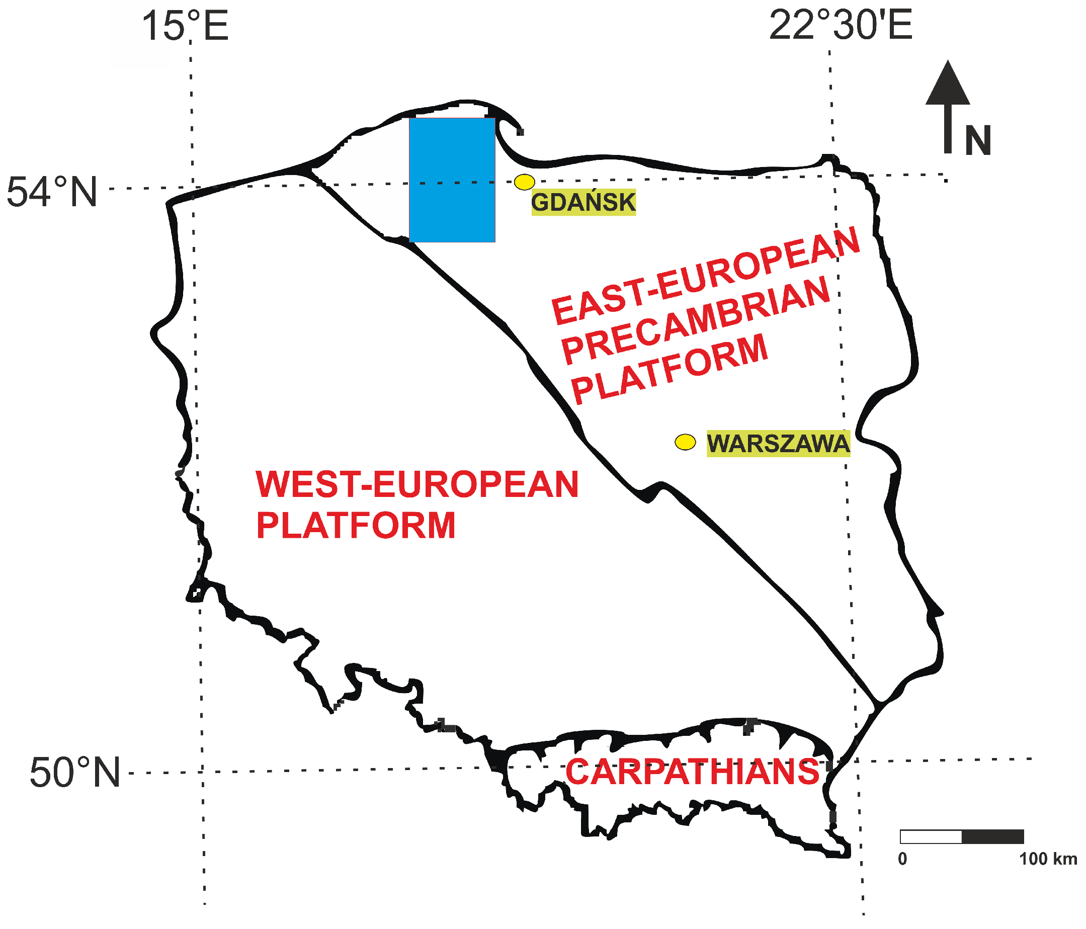
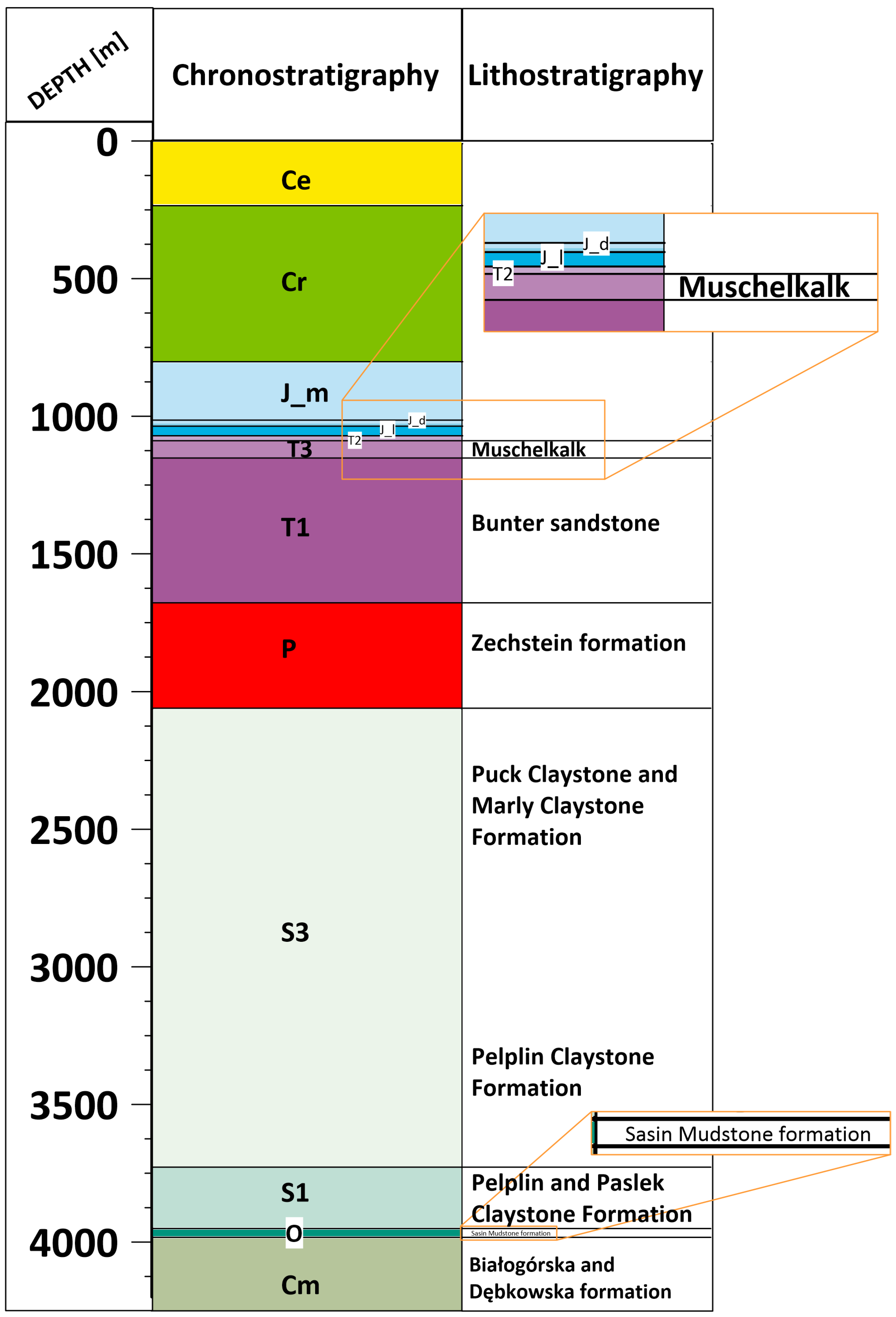
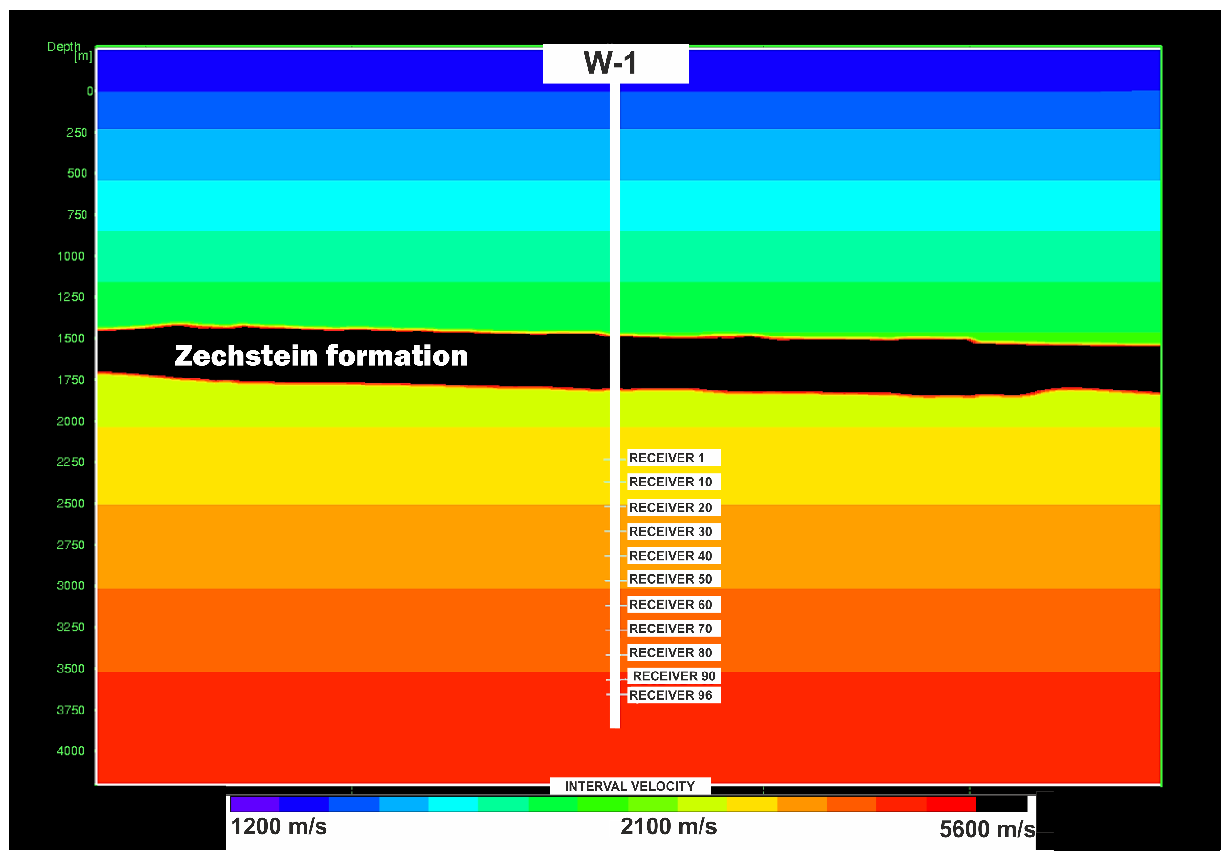
• The receivers were located in the depth interval where seismic imaging produces low-quality results due to the properties of the overburden layers. This is a very well-known exploration problem in northern Poland. The Zechstein formation is mostly made of salts, anhydrite, and dolomite. This complex can be described as a shielding screen for seismic signals. This is believed to be the main cause of the failure of hydrocarbon exploration in this region because sub-Zechstein formations cannot be reliably interpreted [10].
• Artifacts related to acquisition. This group includes weak tool anchoring, which can possibly generate various types of noise (hard to classify) due to pressure and the forces present in the well. The device hung on a cable about 3 km long. Note that noise related to the tool’s resonance is often removed by changing its position and moving it up or down. In this case, the tool was in the same place for the whole acquisition period. Furthermore, in many parts of the well there was no casing between the inner and the outer tubes. Ring noise can be generated when a casing is unbounded.

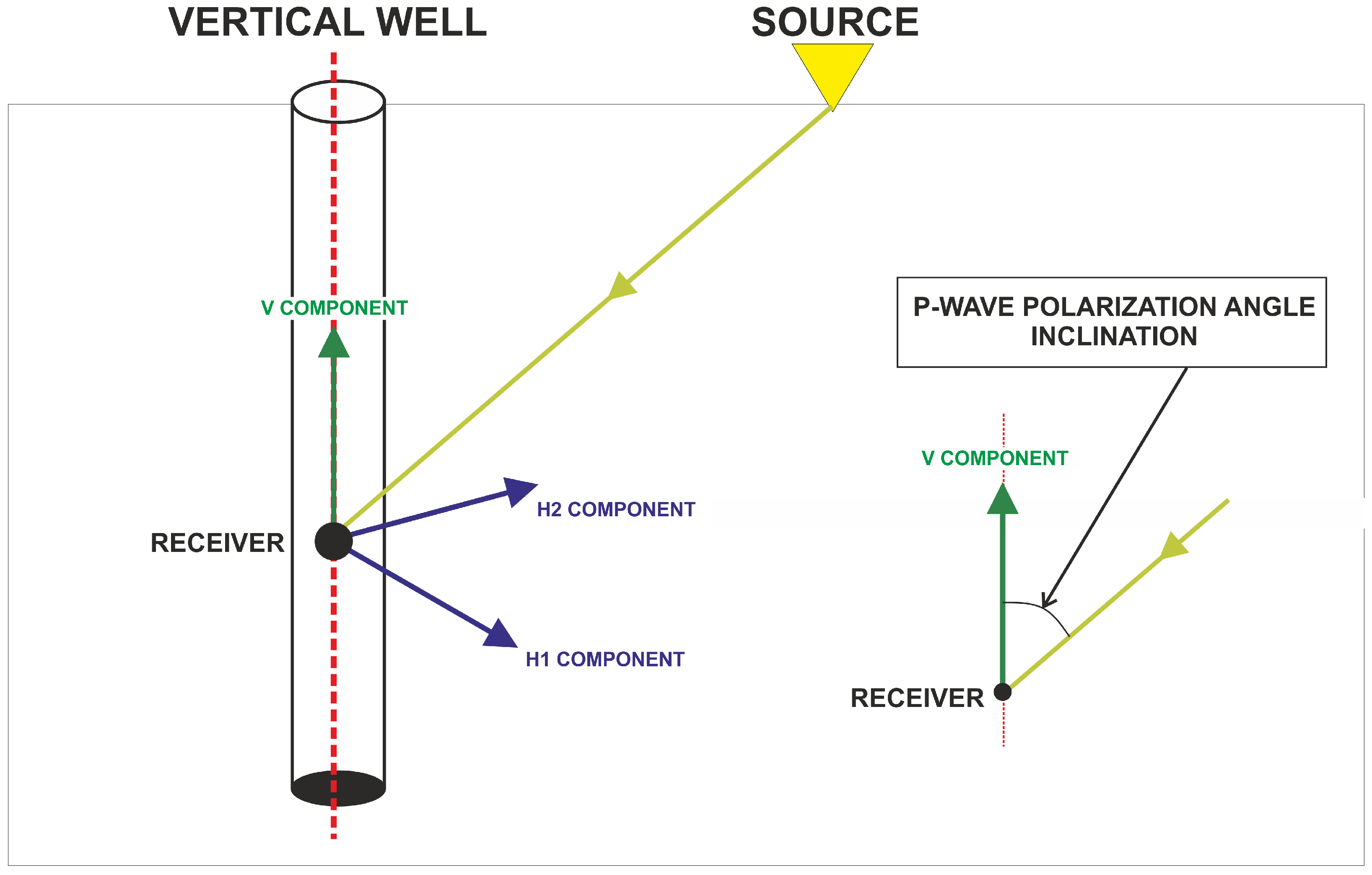
We wanted to examine the best processing workflow for wavefield separation. Typical VSP acquisition consists of 3C receivers that can record two horizontal components (H1 and H2) and one vertical component (V). All components are perpendicular to each other. The correct wavefield separation of the compressional downgoing P-wave on the vertical component and the longitudinal SH and SV waves on the horizontal components is an important seismic processing step. This can be done using the analytical method proposed by Galperin [11], which is based on the directions of the motion of particles. We tested four processing sequences to determine which one allows the best wavefield separation and, consequently, to accurately determine the polarization angles of the longitudinal wave. This is crucial in the case of P-wave inversion, which needs properly estimated polarization angles [4]. We tested the following workflows:

• Workflow 1 (W1)—component rotation on raw data for each shot; vertical stacking; noise attenuation.
• Workflow 2 (W2)—vertical stacking of raw data; component rotation using stacked data; noise attenuation.
• Workflow 3 (W3)—noise attenuation before vertical stacking; component rotation on each shot separately; vertical stacking.
• Workflow 4 (W4)—noise attenuation; vertical stacking followed by component rotation.

Noise attenuation was always the same and consists of the following procedures:

• Single time-invariant, zero-phase Ormsby band-pass filter; frequency range: 16–80 Hz, low-cut: 8 Hz, high-cut ramp: 40 Hz.
• Monofrequency noise attenuation (this type of noise was widely present in these data).
• Time-space frequency filtering using short-time Fourier transform (STFT) for noise related to tool resonance or surface noise passed via the cable. We used a 200 ms window; the aperture was equal to five traces; threshold value: 3; frequency range: 20–80 Hz.
• Vertical and horizontal median filtration for high-energy noise attenuation (a general problem for near-offset shot points). Filter parameters were 100 ms for the vertical window, 30 traces for the horizontal dimension, and 50 ms cosine taper zone; no-scaling factor was used.
• Attenuating energy over first breaks using top mute.

Our processing sequence selection criteria were the lowest polarization angle determination error and the most stable distribution along the whole depth interval. The polarization angle is the angle between the axis of the vertical well (parallel to the receiver’s vertical component) and the P-wave incident ray. We will call this the angle inclination; see Figure 6.

In order to estimate the error of the determination of the polarization angles for each receiver point, the standard deviation of each 5-receiver group was calculated according to Equation (1):

$$\sigma (R_n)=\sqrt{\frac{{\sum }_n^N{(R_n-\overline{R})}^2}{N}},$$

(1)

where $(R_n)$ is inclination value for a particular receiver, $\sigma (R_n)$ is the error for a receiver at depth point n, N is a group of 5 receivers, and $\overline{R}$ is the average value of the inclination angle for this group. Then, the simple arithmetic averages of the standard deviations calculated in the previous step were considered as average errors for each shot point using Equation (2):

$$average error(SP)=\frac{{\sum }_n^{N_E}\sigma (R_n){)}^2}{A_E},$$

(2)

where $A_E$ is the number of estimated angles and $\sigma (R_n)$ is less than $5^0$.

In this step, we decided to use workflow 4, which produced the lowest error. In general, the stacking procedure strengthens the useful signal and reduces random noise. In workflow 4, we first performed noise attenuation procedures to reduce noise, which is not random, and to avoid its possible subsequent reinforcement in the stacking process. We had to take this additional step due to weather and ground conditions. The surface zone changed between sweeps, and the seismic vibrator trucks sank into the water-logged ground. The elevation changes were significant. The first and the last sweep in each shot point were performed under different geotechnical conditions. Pore space decreased as a result of compaction; as a consequence, the amount of water filling these pores also changed. To make sure that vertical stacking in this situation would in fact help to reduce unwanted interference and strengthen the useful signal, we decided to add a signal-matching procedure before stacking. We know a priori from 3D seismic surface surveys that anisotropy strength is very low. The observed anisotropy is at the limit of detection by seismic methods (${10}^{-3}$ to ${10}^{-2}$). The combination of the great depth and very small values of parameters forced us to obtain the most accurate polarization angles without additional distortions caused by the conditions under which the acquisition was performed. Before we decided to use a time-frequency matching filter, we performed a correlation between records with the calculated reference record (the average of all sweeps on the shot point), see Figure 7.

At the beginning of the examined depth interval, we can see the lowest correlation for all sweeps. This is an expected effect, as there was no casing between the $9^{″}$ and the $7^{″}$ tubes in this part. In the rest of the well, where casing is present, we can see significantly higher correlation, except for the 3200–3400 depth interval, where the correlations are weaker. This is probably due to weak anchorage of receivers in this part of the well; however, this is also a change zone between the Ludlow and upper Silurian complexes.

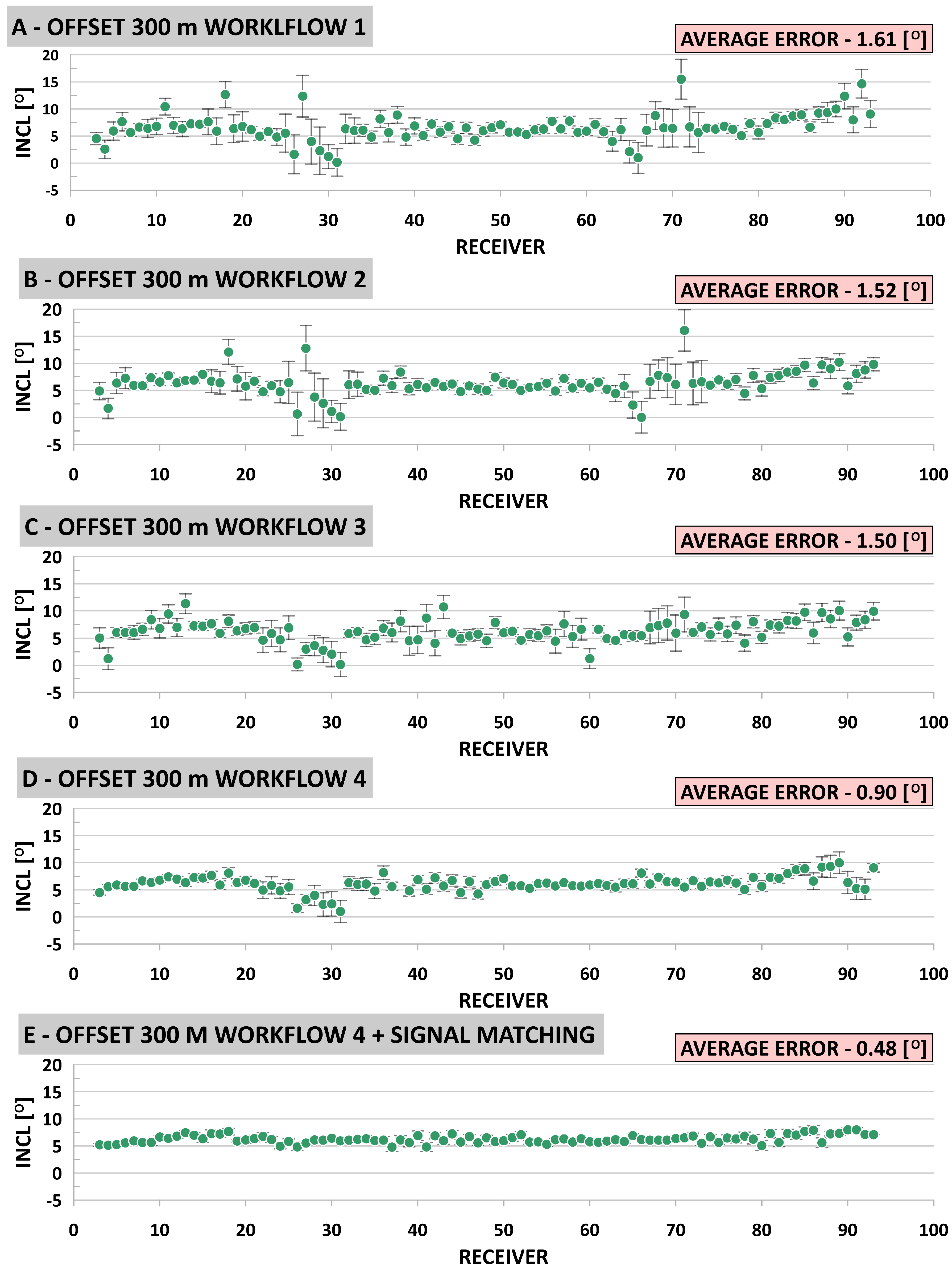
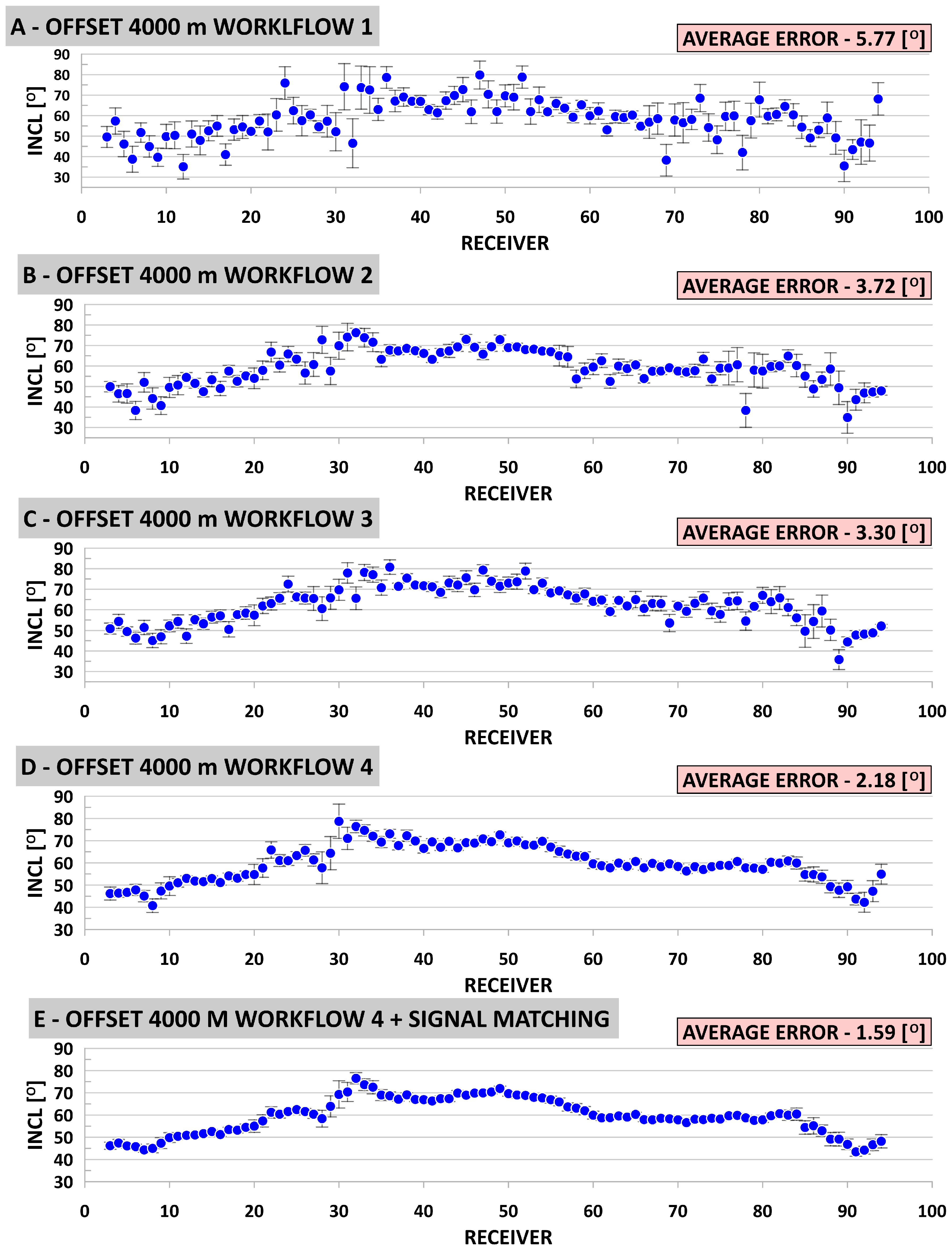
To evaluate this methodology, we plotted estimated inclinations for near-offset SP in Figure 8 (offset 300 m) and for far-offset SP in Figure 9 (4000 m). In both cases, the lowest average error was obtained using workflow 4 with the additional signal-matching procedure. For both offsets, the least optimal workflow was workflow 1 because the Principal Components Method (PCM), which we used for component rotations, needs the first-break times on its input. In this step, the downgoing P-wave energy is used. The window that defines this energy should be centralized around the first-break time. In workflow 1, the first step was first-break picking. We performed hand picking because it was impossible to use an automatic picker due to noise. Performing first-break picking on this step is not very accurate due to the interference between the signal and the noise. These phenomena can lead to changes in the maximum and minimum amplitude position of the signal. This, on the other hand, may cause incorrect determination of the first-break times. Workflow 2 has a slightly lower error than workflow 1 because vertical stacking reduces some random noise; as a result, the first-break picking accuracy can be higher. However, this error increases with the offset. For near-offset shot points, the relative change of average error is not as significant as for shot points located in the far offsets. For the 300 m offset, the average error of workflow 2 is approximately 6% lower compared to workflow 1, while for the 4000 m offset there is a 35% difference. Data processed using workflow 3 have a smaller error compared to data from workflows 2 and 3. The smallest error was obtained using workflow 4. Importantly, adding a matching filter to the workflow with the lowest average error significantly improved the inclination estimation. Compared to workflow 1, the average error reduction for workflow 4 with the signal-matching procedure applied is approximately 71% lower for the near-offset shot point, and it is 83% lower for the far-offset shot point. In the case of original workflow 4, adding the signal-matching procedure resulted in 47% lower error for the near offset and 37% lower error for the far offset. 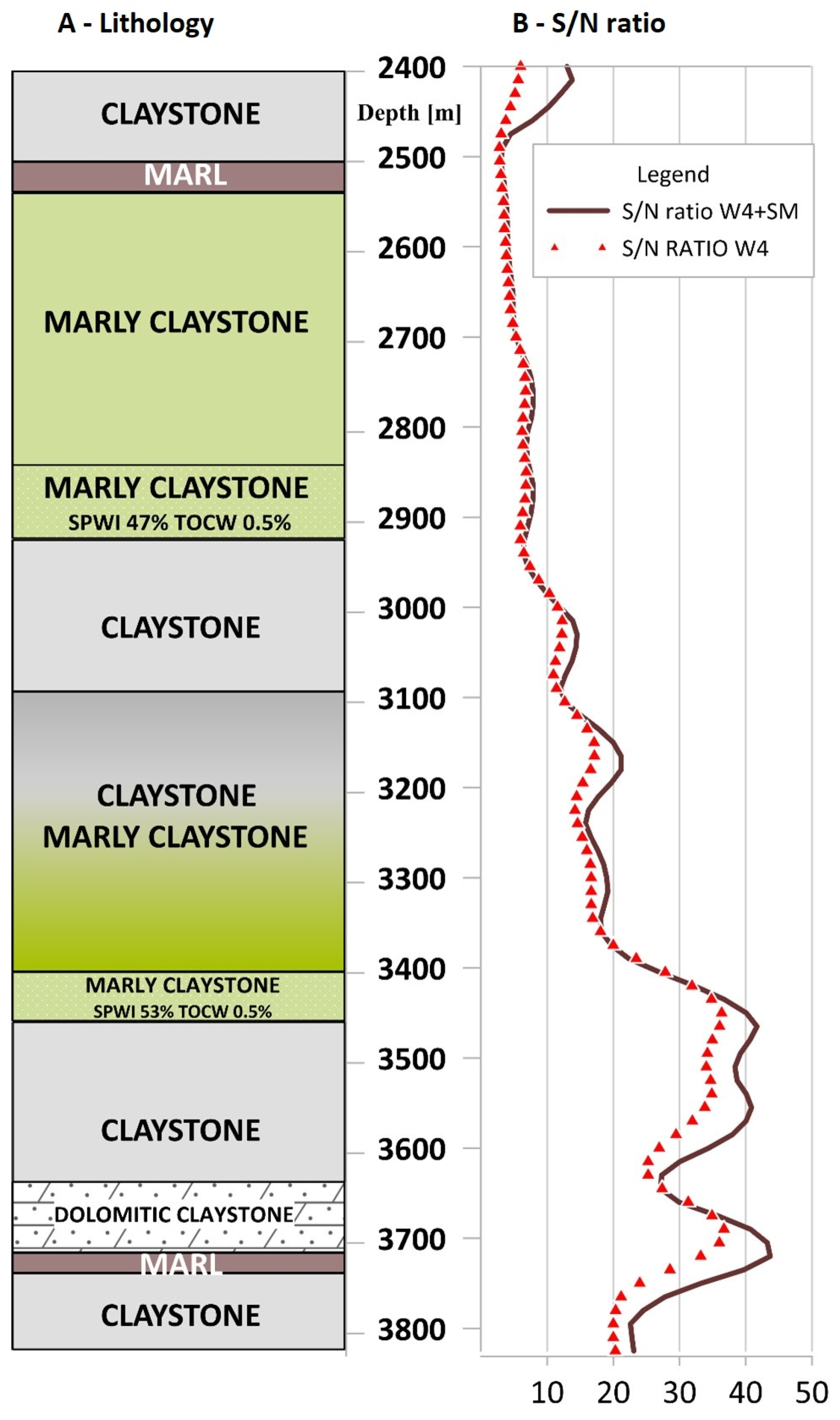Figure 10 shows a comparison between the S/N ratio for workflow 4 and workflow 4 with the signal-matching procedure with reference to the lithostratigraphic column. We can see a similar phenomenon as in Figure 6: a lower S/N ratio in the depth interval where there is no casing between the inner and the outer tube. The significantly greater value of the S/N ratio can be seen in the Ludlow depth interval. This geological complex is built of marly claystone with SPWI 53%, then marl and claystone on the bottom. Note that the signal-matching procedure improved the S/N ratio, which is important for component rotation and, consequently, also for estimation of inclination angles. 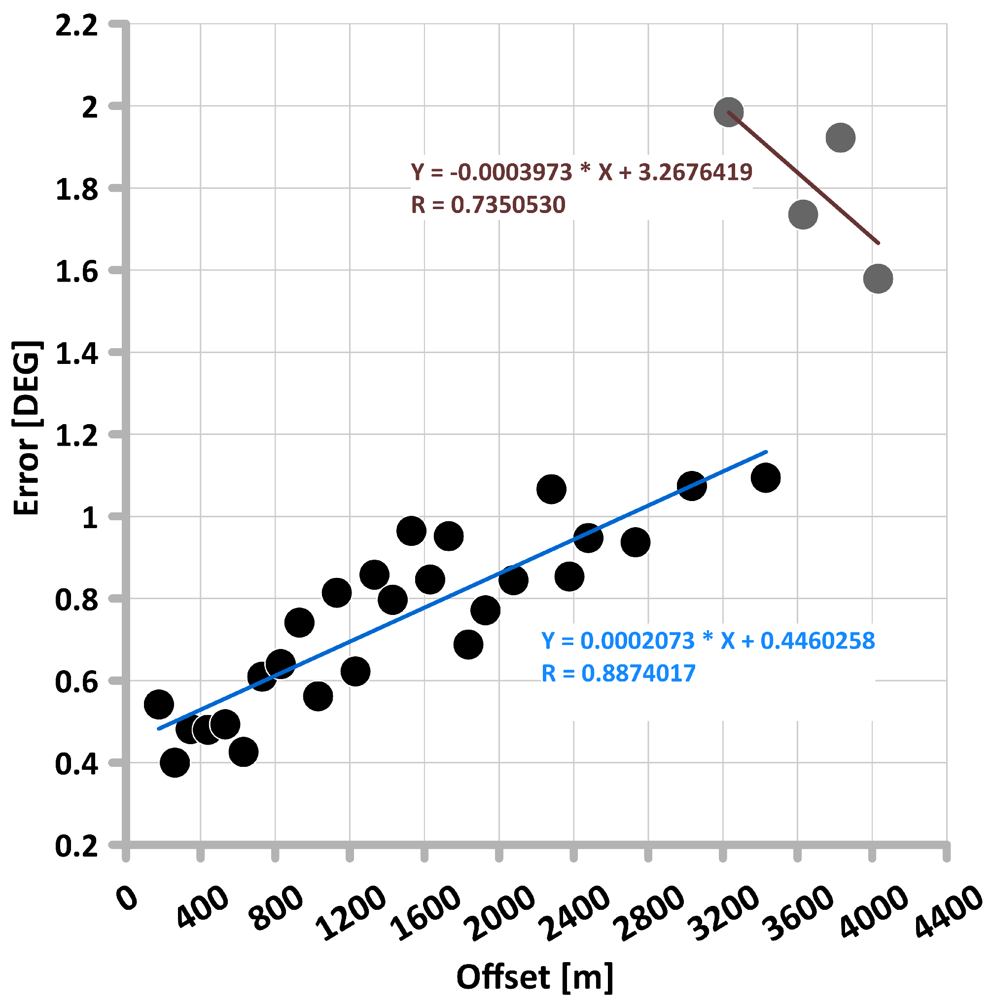Figure 11 shows a plot of average errors (y axis) for workflow 4, and the signal-matching procedure against the offset (x axis). It can be seen that the error increases linearly as the offset increases. However, there are two groups: the first is from the beginning to the offset at approximately 3200 m, and the second group is from the offset at 3200 m to the offset at 4400 m. The first group has a strong positive linear trend and the error varies from 0.3 to 1.2, while the second group shows a negative linear trend. The highest error value is 2 for the smallest offset of this group; as the offset decreases, the error also subsequently decreases to a value of 1.6. However, there are not enough points to fully interpret this phenomenon. The reason for this is probably related to the aforementioned acquisition problems. The final field report states that some far offset points were skipped because the data quality was below the acceptance level and the ground conditions. 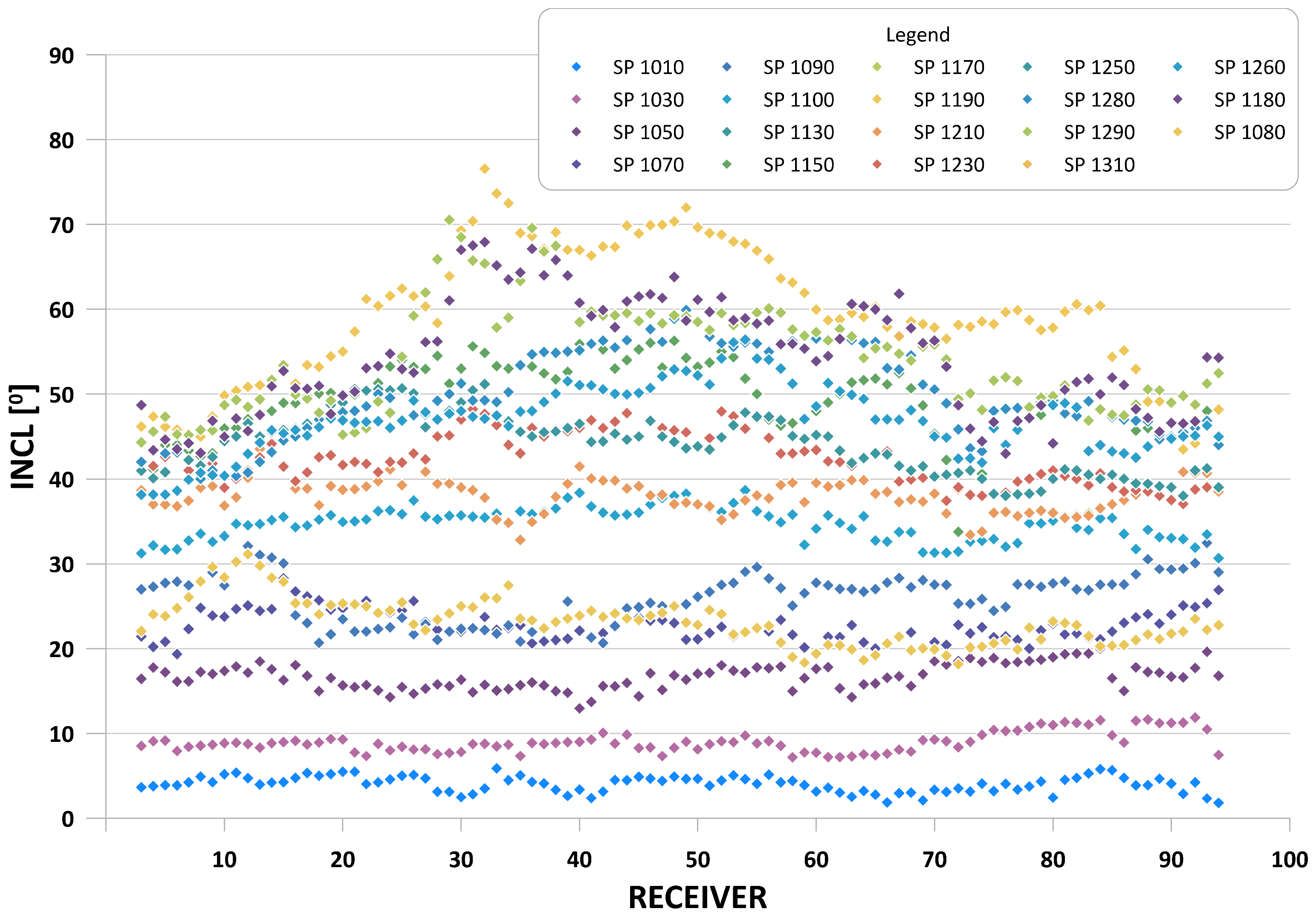Figure 12 shows inclination distributions for the different offsets used for further calculations for estimation of anisotropy parameters.

4. Local Anisotropy Estimation

Several methods allow the determination of anisotropy based on VSP data including slant stack [12], slowness [13], and slowness-polarization method [4]. We used the slowness-polarization method described by Grechka and Mateeva [4] because information about polarizations stabilizes the solution and simplifies the inversion process [4]. Additionally, we wanted to obtain anisotropy parameters at a given depth without entering layer boundaries and any additional assumptions beforehand. Grechka and Mateeva used this methodology for 2D walkaway VSP data gathered in the Gulf of Mexico, where receivers were partially placed inside salt. They proved that estimated in situ anisotropy coefficients can be correlated with lithology and other geophysical methods such as gamma-ray measurement. In the case of vertical transverse isotropy (VTI) media, Grechka and Mateeva speculated that parameter $\eta$ (Alkhalifah and Tsvankin’s anellipticity coefficient [14]) could be slightly less correlated to the lithology than $\delta$ (Thomsen’s anisotropic coefficient [15]). This is mostly because of the dependence of $\eta$ on local stress anomalies. Our goal was to show that this methodology can be used even if anisotropy is extremely small. Grechka and Mateeva [4] worked with data acquired in a medium with an anisotropic complex beneath salt and almost isotropic salt. This paper presents the equations necessary to perform the inversion. A detailed mathematical and theoretical description of this method is presented in the appendices of Grechka and Mateeva’s paper [4]. The slowness-polarization method starts from the weak-anisotropy approximation. Each time we refer to $V_p$ and $V_s$ in Equations (3)–(19), we mean vertical P and S velocity. In the case of a VTI medium, it can be described by Equation (3) using vertical slowness (q), P-wave inclination angle ($\alpha$), $\delta$ anisotropic coefficient [15], $\eta$ anellipticity coefficient [14], and $V_p$ velocity. The P-wave slowness polarization vector p component is then described by

$$p_3\equiv q(\alpha )\simeq \frac{cos(\alpha )}{V_p}·(1+{\delta }_{VSP}·{sin}^2(\alpha )+{\eta }_{VSP}·{sin}^4(\alpha )),$$

(3)

where $\alpha$ is the inclination angle.

In the case of a VTI medium and measurements in a vertical well, the anisotropic dependence q($\alpha$) is controlled by ${\delta }_{VSP}$ (more sensitive to near-offset q($\alpha$) variations) and ${\eta }_{VSP}$ (more sensitive to far-offset q($\alpha$) variations), see Equations (4)–(6):

$${\delta }_{VSP}=(f_0-1)\delta ,$$

(4)

$${\eta }_{VSP}=(2f_0-1)\eta ,$$

(5)

$$f_0=\frac{1}{1-\frac{V_S^2}{V_P^2}}.$$

(6)

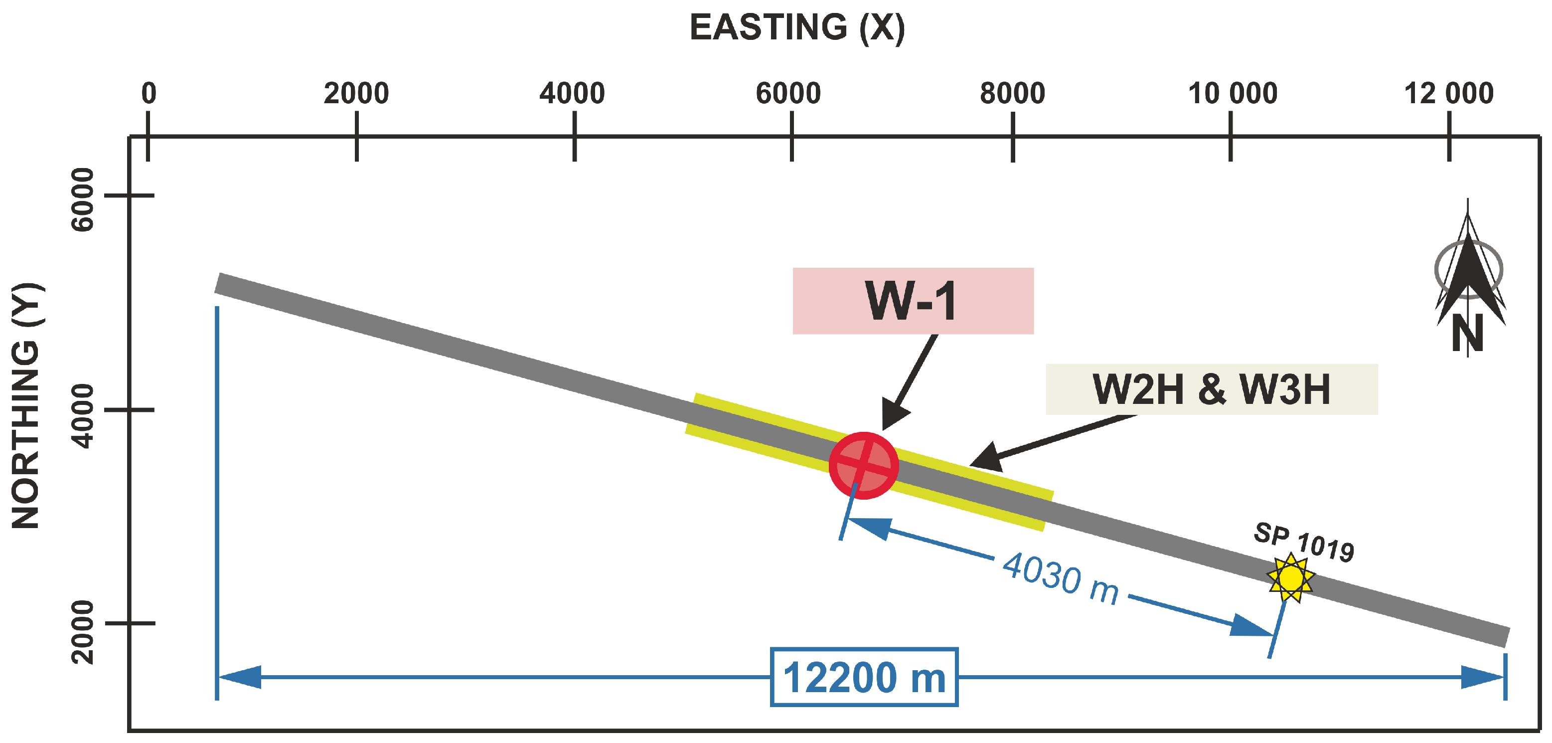
If one wants to invert directly for $\eta$ and $\delta$, the $p_v$ ratio has to be known beforehand. The average value of $V_S$/$V_P$ in Well W-1 is 0.54, therefore the average $p_v$ is 0.29 according to Equation (7):

$$p_v=\frac{V_S^2}{V_P^2}.$$

(7)

Using Equation (7), $f_0$ can be described by

$$f_0=\frac{1}{1-p_v}\approx 1+p_v.$$

(8)

The approximation in Equation (8) is used only for the sake of simplification, presenting the theoretical relationships between the parameters ${\eta }_{VSP},{\delta }_{VSP}$, and $\eta ,\delta$. In fact, we are calculating the $f_0$ directly in every depth point.

Finally, Equation (3) can be written using $p_v$ in Equation (9):

$$q(\alpha )\simeq \frac{cos(\alpha )}{V_p}·(1+p_v\delta ·{sin}^2(\alpha )+(1+2p_v)\eta ·{sin}^4(\alpha )).$$

(9)

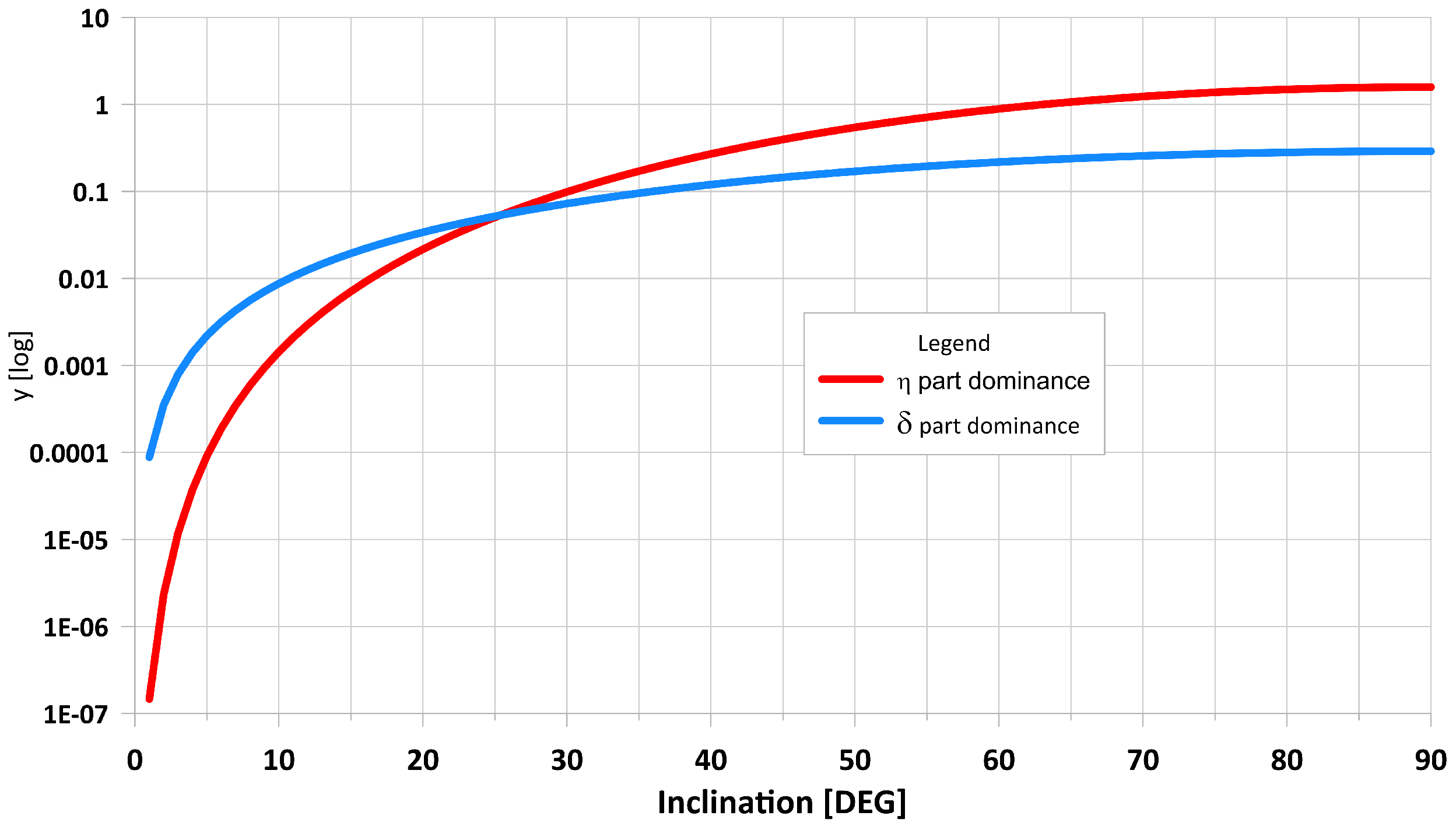
To better understand the dependencies of $q(\alpha )$ and ${\eta }_{VSP}$ with ${\delta }_{VSP}$ on the offset, an average $p_v$ value of 0.29, and (1 + 2$p_v$) equal to 1.58, the dependency graph is shown in Figure 13.

Figure 13 shows that average polarization angles below 25° are for shot points numbered 1010 to 1180, which correspond to an offset from 0 to 1700 m, and in this range the polarization vector is mostly influenced by the $\delta$ part in Equation (9). For offsets from 1700 to 4000 m, the polarization vector is mostly influenced by $\eta$ (angles over 25°). Thus, it is obvious that for reliable inversion a wide spectrum of polarization angles is needed. The theoretical minimum of $\delta$ can be calculated using the following equation ([16]):

$${\delta }_{min}=-\frac{1}{2f_0}.$$

(10)

which is equal to −0.7034 with an average $p_v$ of 0.28. For the inversion, we need to specify the parameters that will be estimated. These parameters are stored in the vector k:

$$\mathbf{k}=[V_P,{\delta }_{VSP},{\eta }_{VSP}].$$

(11)

Vertical $q^{calc}(k,\alpha )$ is calculated without weak anisotropy approximation, directly from Equations (12)–(15):

$$\mathbf{I}=\left[\begin{array}{c}sin(\alpha )\\ 0\\ cos(\alpha )\end{array}\right],$$

(12)

$$\mathbf{p}=\frac{1}{V(\theta )}\left[\begin{array}{c}sin(\theta )\\ 0\\ cos(\theta )\end{array}\right].$$

(13)

where $\mathbf{I}$ is polarization vector, $\mathbf{p}$ is slowness vector, $\theta$ is polar phase angle, and V($\theta$) is the phase velocity of the P-wave. Now, using Christoffel’s equation and the Voigt notation for stiffness coefficient $c_{ij}$, the relation between $\theta$ and $\alpha$ can be estimated using Equation (14) (see in [4], Appendix B):

$$\left[\begin{array}{cc}{c}_{11}{sin}^2(\theta )+c_{55}{sin}^2(\theta )-V^2& (c_{13}+c_{55})sin(\theta )cos(\theta )\\ (c_{13}+c_{55})sin(\theta )cos(\theta )& c_{55}{sin}^2(\theta )+c_{33}{sin}^2(\theta )-V^2\end{array}\right]\times \left[\begin{array}{c}sin(\alpha )\\ cos(\alpha )\end{array}\right]=0.$$

(14)

When $c_{13}$ + $c_{55}$ is not 0, the phase velocity is equivalent to the same wave mode. Solving the linear equation by eliminating variable V results in the following:

$$(c_{11}-c_{55})t{g}^2(\theta )+2((c_{13}+c_{55})ctg(2\alpha )tg(\theta )-(c_{33}-c_{55})=0.$$

(15)

Considering anisotropic rocks, we know that the equation has two roots because $c_{11}$ > $c_{55}$ and $c_{33}$ > $c_{55}$ in this medium. These roots correspond to the phase angle whose difference between the polarization angle of the P and SV wave is the smallest. The phase velocity is a square root of the Christoffel equation’s greatest eigenvalue, therefore $p(\alpha )$ can be calculated using Equation (13). The last step is to minimize the objective function by changing the values of the elements of vector k:

$$F(k)=\sum \frac{{[{\mathbf{q}}^{calc}(\mathbf{k},\alpha )-\mathbf{q}(\alpha )]}^2}{{\sigma }^2},$$

(16)

where ${\sigma }^2$ describes the errors, which are estimated using the following equation:

$${\sigma }^2={\sigma }^2(\mathbf{q})+{(\frac{sin(\alpha )}{<V_P,log>})}^2{\sigma }^2(\alpha ),$$

(17)

where $<V_p,log>$ is the P-wave velocity from the sonic tool. The minimization process of function $F(k)$ starts from an isotropic medium assumption, where vector k is equal to

$$\mathbf{k}=(V_P,0,0).$$

(18)

$V_P$ is calculated using

$$V_P=\frac{{\sum }_n^N\frac{{cos}_n(\alpha )}{q_n(\alpha )}}{N},$$

(19)

where N is the number of the considered depth points.

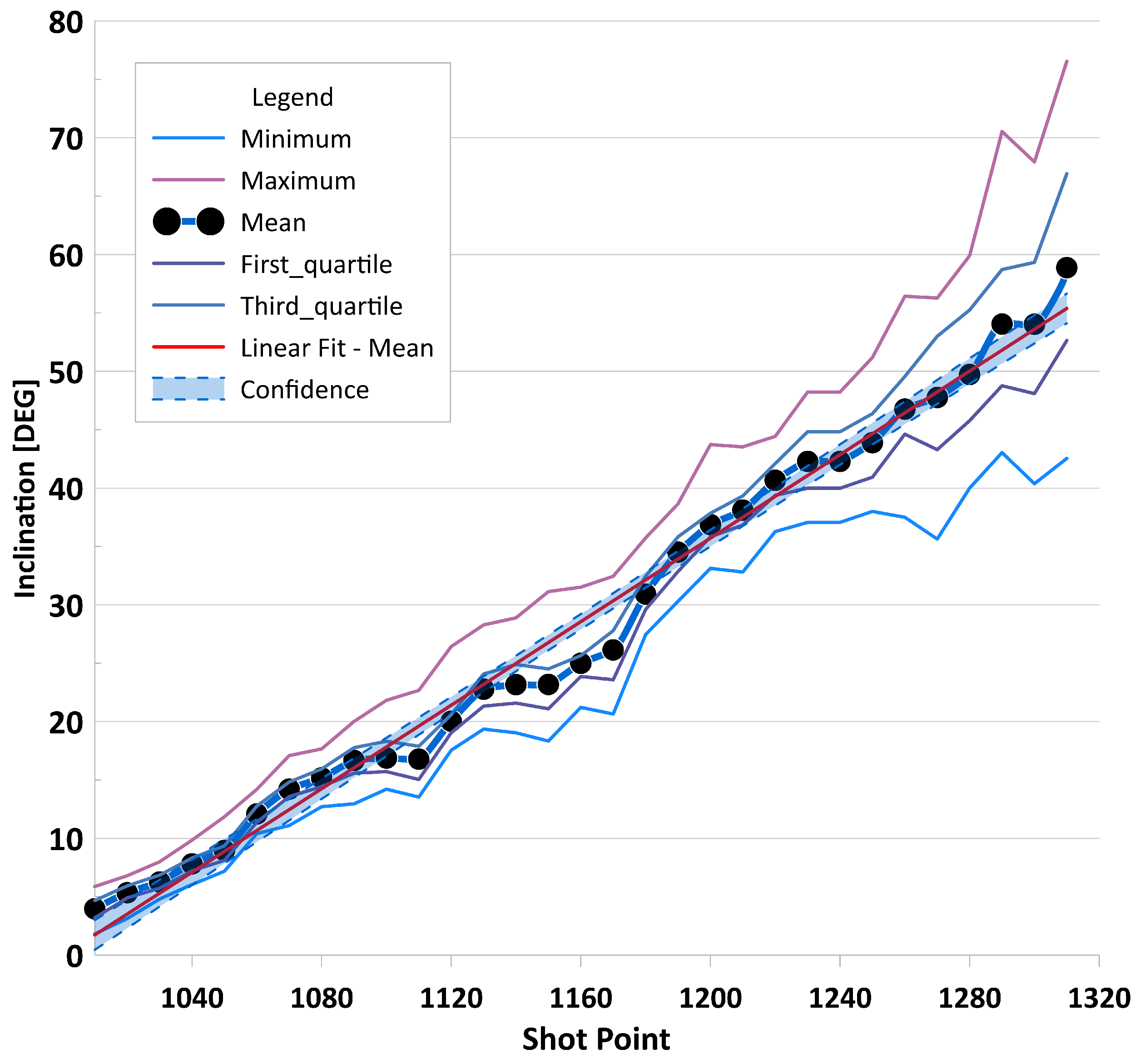
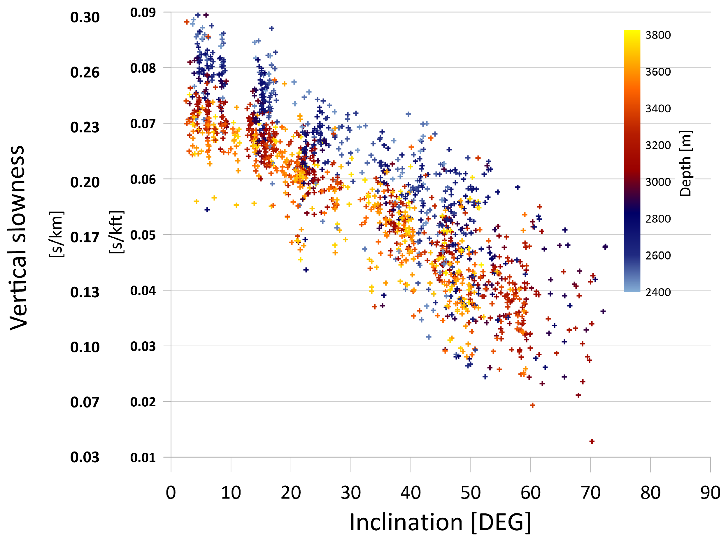
Estimated average P-wave polarization angles for the different shot points along the profile and errors of their estimation (calculated according to Equation (2)) are characterized by a stable linear increase with offset, which is visible in Figure 14. Two areas that deviate from the trend line can be found: one around shot point 1120 (offset around 1230 m) and the other around shot points 1140–1180 (offset 1400–1800 m). We can assume that this is because vibrator trucks did not reach the designated points on the profile. Therefore, they were moved to other locations close to those points but not on the profile line. Another reason could be related to record quality. Besides the observed deviation, we decided to use these data for the anisotropy calculation. In Figure 15, the vertical slowness versus offset graph is presented for all offsets and depth points. Colors represent different depth points. It can be seen that depending on the depth, the difference in elastic properties is obvious. The downward shift along the Y-axis is caused mostly by the velocity increase with depth because Equations (3) and (9) contain the component $\frac{cos(\alpha )}{V_p}$, by which the whole equation is multiplied. 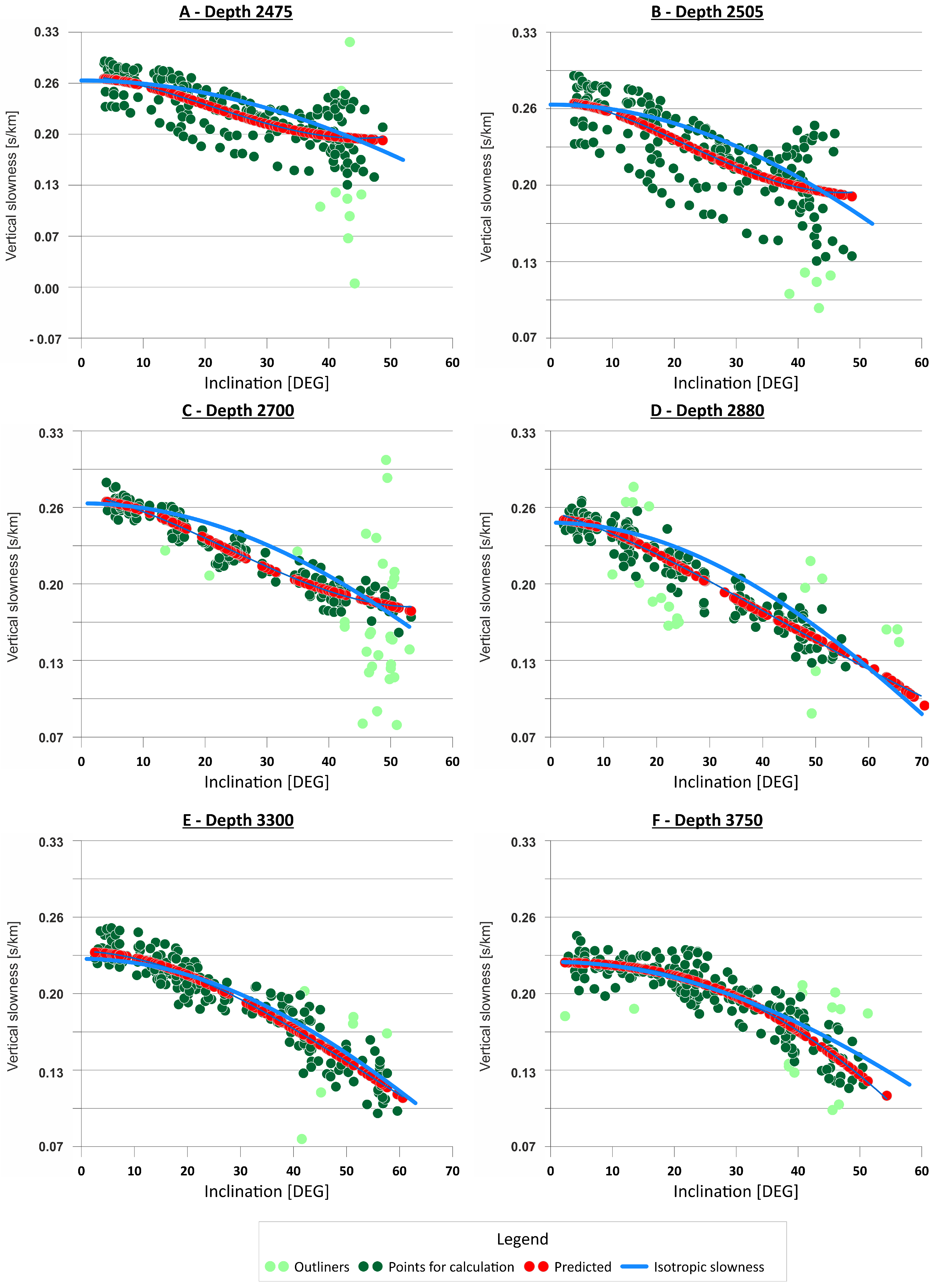Figure 16 shows a vertical slowness polarization graph for six depth intervals: 2475, 2505, 2700, 2880, 3300, and 3750 m. Green points (dark and light ones) represent all data prepared for the inversion process before validation. Dark green points were used for inversion calculation, and red represents the predicted values. The blue line is calculated according to the assumption that the geological medium is isotropic. For a depth interval of 2880 m, which reaches the top of the marly mudstone layer and is potentially saturated with gas, there is a noticeable shift between the predicted points and the calculated isotropic vertical slowness line from angle 10°. As mentioned before, for inclinations over 25° the $\eta$ parameter dominates the solution of the slowness-polarization equation. Figure 16 presents raw estimated parameters ($\delta$, $\eta$) with no smoothing after inversion. Both parameters reach their absolute maximum at depth point 2880. At depth points 2475 (Figure 16A) and 2505 (Figure 16B), a similar shift can be observed between the isotropic vertical slowness line and the predicted points. The absolute values of the estimated parameters reach their maximum before a rapid change to almost zero. This change can be observed on the border between claystone and the very thin marl layer. Jakobsen and Johansen [17] made a detailed anisotropic approximation in their research on mudrocks. They showed that a negative value of $\delta$ is observed in specific kinds of mudrocks. Additionally, they ran a simulation of in situ stress in this kind of rock and examined its impact on Thomsen’s parameters, and the values of $\delta$ were negative. In Figure 16C, at depth 2700 m the shift between the predicted values and the isotropic curve can be seen; again, it is more noticeable for angles over 10°. This is the center of another claystone layer (bottom 2850 m). We can observe similar values of $\delta$ and $\eta$ as in the first claystone layer. Then (Figure 16D), at depth 2880 in the thin layer of saturated marly claystone, the separation between the isotropic vertical slowness line and the predicted values increases, and the anisotropic parameters have higher absolute values. Going down from depth 2950 to 3400, the thin layer of claystone sits on a thicker layer of claystone and marly claystone. In the clear claystone layer (bottom of the layer at depth 3100 m), $\delta$ and $\eta$ have similar values as in the previous claystone layers. In the layer where claystone transitions into marly claystone, the anisotropic parameters’ values become closer to zero. This effect can be observed in Figure 16E, in which the isotopic vertical slowness line crosses the predicted points. A change from negative to positive values in both parameters can also be seen where the marly claystone transitions into dolomitic claystone. In Figure 16F, the theoretical isotropic vertical slowness line passes through the center of the predicted points. Again, this is a very thin marl layer where $\delta$ and $\eta$ are close to zero. These results clearly show that the presented P-wave-only VSP data inversion methodology can be used for lithology studies. Moreover, the estimated anisotropic parameters are reliable and can be used even if the elastic anisotropy of the geological medium is relatively small (on the limit of detection by surface seismic methods). Bandyopadhyay [18] showed that in a laminated geological medium, the sign of Thomsen’s parameters can be used as fluid identification, and small values of Thomsen’s parameters could be related to the compaction regime.

We also calculated the following parameters: $V_r$, which is used as a lithology identifier (Equation (20)), and Poisson’s ratio using Equation (21). We decided to plot it against the parameters estimated from VSP inversion to analyze its relative change according to the lithology and to compare the sensitivity of these parameters to lithological changes. Thomsen [15] proved that $V_r$ can be used for lithology correlation in rocks with transverse isotropy. Ryan Grigor in 1997 [19] came to similar conclusions. For an isotropic medium, the $V_r$ should directly depend on changes in the Poisson’s ratio, which is unique [20]. This factor is not unique for an anisotropic medium [21].

$$V_r=\frac{<V_P,log>}{V_{SX}},$$

(20)

where $V_p$ is sonic P-wave velocity and $V_{SX}$ is sonic wave velocity from horizontal X-component.

In the case of well W-1, it does not matter whether $V_{SX}$ or $V_{SY}$ (from the sonic tool) was selected for the calculations as they are almost equal to each other. The average $V_{SY}/V_{SX}$ ratio for the whole investigated depth range is 0.9987.

$$POISSON RATIO=\frac{V_r^2-2}{2V_r^2-2}.$$

(21)

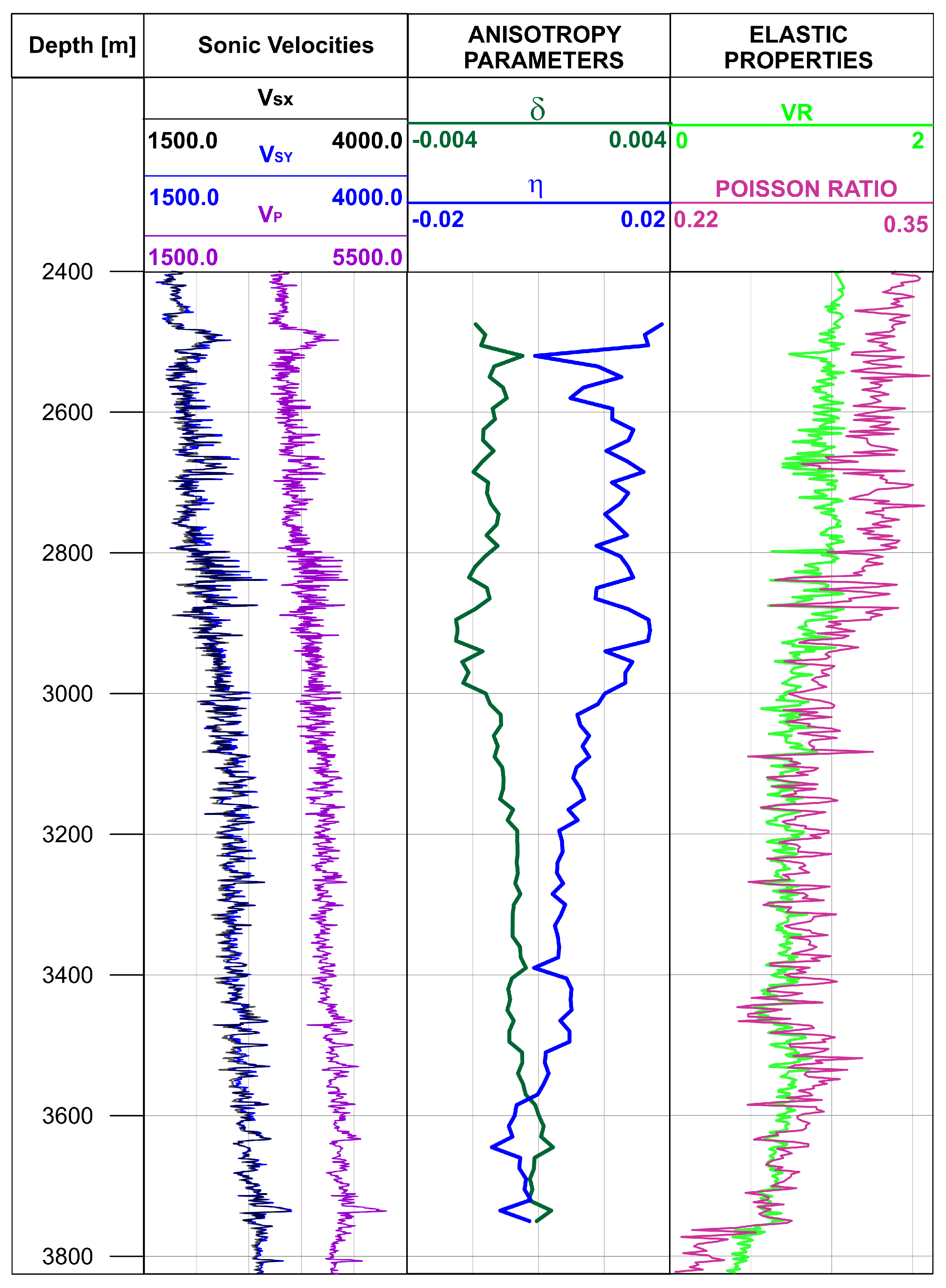
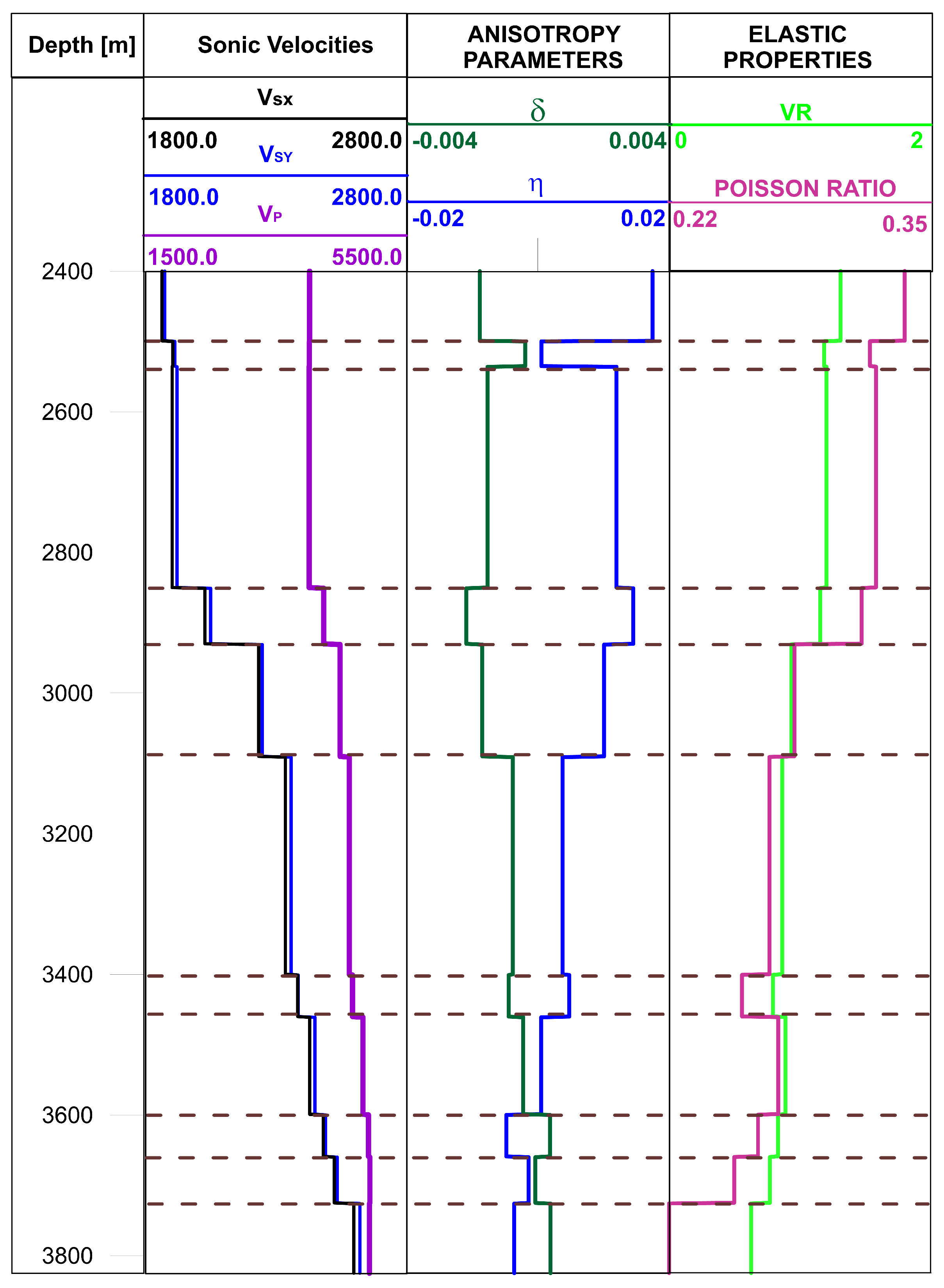
Figure 17 shows sonic $V_{SX}$, $V_{SY}$, $V_P$ velocities; $\delta$ and $\eta$ from VSP inversion; and $V_r$ with Poisson ratio. Figure 18 shows the same parameter set averaged to the single value in the layers. In the first marl layer, rapid changes in $\delta$ and $\eta$ are clearly visible, whereas the other parameters remain stable. A similar situation is observed in the thin marl layer located at a depth below 3700 m. Again, there is almost no change in $V_{SX}$ and $V_P$ velocity. A similar situation can be noticed in saturated marly claystone. The relative change in VSP anisotropic parameters is more visible than in $V_r$. The change in the sonic velocities is noticeable, but their ratio remains almost unchanged. An interesting phenomenon can be observed when claystone transitions into dolomitic claystone, where the signs pf the parameters $\delta$ and $\eta$ change. In Jakobsen and Johansen’s [17] laboratory studies on the anisotropy of mudrocks, positive $\delta$ was present in the rocks with low porosity, while negative values were related to higher porosity value.

5. Discussion

The P-wave-only inversion of the walkaway VSP data method introduced by Grechka and Mateeva [4] showed good results for local anisotropy estimation on the dataset, with a strong contrast between the near-isotropic salt overburden and sediments with significant anisotropy beneath it. We used this methodology for a very complex survey that was performed in one of the first exploratory wells for shale gas exploration in Poland. We had a priori knowledge about the very low seismic anisotropy strength and the estimated values of Thomsen parameters used for depth migration. Helbig and Thomsen [22] showed the importance of low anisotropy in modern exploration. Accuracy analysis of small seismic anisotropy is crucial to improve surface seismic processing and interpretation. It allows negative effects of noise attenuation to be reduced as well as better coherency and velocity analysis [22]. In this paper, we showed that these parameters can be estimated from a walkaway VSP survey even if the anisotropy strength from the surface seismic survey is calculated to be 2–4%.

These challenging acquisition and workflow tests show that choosing the proper processing scheme is crucial for reliable estimation of polarization angles. We tested four different processing workflows to meet Grechka and Mateeva’s [4] criterion for the accuracy of polarization measurements. As the acquisition itself was carried out in problematic conditions that potentially hindered the seismic signal, and the anisotropy of rocks in this place is low, we faced the difficult task of reconstructing the anisotropy parameters. The seismic signal in the case of VSP acquisition goes through the near-surface zone (NSZ) only once; however, in surface seismic surveys the signal travels twice through the NSZ. This zone is one of the most detrimental for seismic signals due to the very low compaction, intensive weathering processes, often-varying rock types, and the complex geology of this zone [23]; however, in this case we observed significant changes in the NSZ zone between sweeps. In this workflow, the first step was noise attenuation, then signal-matching was applied before vertical stacking, and the last step was component rotation; this is the most appropriate method in cases of inclination estimation errors.

The estimated $\delta$ and $\eta$ parameters from walkaway VSP are low: −0.003 < $\delta$ < 0.001 and −0.01 < $\eta$ < 0.02; however, their relative changes are strongly correlated with lithology. The behavior of $\delta$ and $\eta$ corresponds to other research done for similar rock formations. Estimated anisotropy parameters from VSP show better correlations with lithology than lithology identifier $V_r$, which was calculated from data from a sonic tool. This is because this sonic tool takes measurements directly in the well, while VSP allows investigation of a larger area whose size is dependent on the offset range. From an offset of approximately 1700 m, parameter $\eta$ clearly dominates in the solution. Parameter $\delta$ dominates in the solution for offset 0–1700 m.

6. Conclusions

This research shows that inversion of P-wave-only data from walkaway VSP surveys can be applied when the geological medium is characterized by very small anisotropy. Additionally, the estimated parameters can be used together with $V_r$ for lithology identification. The sensitivity of VSP anisotropic parameters to lithological changes is higher than the sensitivity of parameters from well logs. In the case of challenging acquisition, when the near-surface zone changes significantly between subsequent sweeps on the same shot point, a special seismic signal processing approach is needed. When workflow 4 is extended with the signal-matching procedure, this allows a significant reduction in the estimation errors of polarization angles.

References

1. Soni, A.; Verschuur, D.J. Full-wavefield migration of vertical seismic profiling data: Using all multiples to extend the illumination area. Geophys. Prospect. 2014, 62, 740–759. [Google Scholar] [CrossRef]
2. Steward, R. VSP: An In-Depth Seismic Understanding. Recorder 2001, 26, 1–13. [Google Scholar]
3. Dewagan, P.; Grechka, V. Inversion of multicomponent, multiazimuth, walkaway VSP data for the stiffness tensor. Geophysics 2003, 68, 1022–1031. [Google Scholar] [CrossRef]
4. Grechka, V.; Mateeva, A. Inversion of P-wave VSP data for local anisotropy: Theory and case study. Geophysics 2007, 72, 69–79. [Google Scholar] [CrossRef]
5. Zaręba, M.; Danek, T. VSP polarization angles determination: Wysin-1 processing case study. Acta Geophys. 2018, 66, 1047–1062. [Google Scholar] [CrossRef]
6. Hawkins, K.; Leggott, R.; Williams, G.; Kat, H. Addressing anisotropy in 3D pre-stack depth migration: A case study from the Southern North Sea. Lead. Edge 2001, 20, 528–543. [Google Scholar] [CrossRef]
7. Kondracki, J. Regional Geography of Poland; WN PWN: Warszawa, Poland, 2011. [Google Scholar]
8. Kasperska, M.; Marzec, P.; Pietsch, K.; Golonka, J. Seismogeological model of the Baltic Basin. In Opracowanie Map Zasięgu, Biostra-Tygrafia Utworów Dolnego Paleozoiku Oraz Analiza Ewolucji Tektonicznej Przykrawędziowej Strefy Platformy Wschod-Nioeuropejskiej Dla Oceny Rozmieszczenia Niekonwencjon-Alnych Złóż Węglowodorów; Golonka, J., Bębenek, S., Eds.; Wydawnictwo Arka: Cieszyn, Poland, 2017. (In Polish) [Google Scholar]
9. Kasperska, M.; Marzec, P.; Pietsch, K.; Golonka, J. Seismo-geological model of the Baltic Basin (Poland). Ann. Soc. Geol. Pol. 2019, 89, 195–213. [Google Scholar] [CrossRef] [Green Version]
10. Bajewski, L.; Wilk, A.; Urbaniec, A.; Barton, R. Improving the imaging of under-Zechstein structures based on the reprocessing of 2D seismic in the West Pomerania region. NG 2001, 4, 195–204. [Google Scholar] [CrossRef]
11. Galperin, E.I. The Polarization Method of Seismic Exploration; Springer: Dordrecht, The Netherlands, 1984. [Google Scholar]
12. Hake, H. Slant stacking and its significance for anisotropy. Geophys. Prospect. 1986, 34, 595–608. [Google Scholar] [CrossRef]
13. Miller, D.; Spencer, C. An exact inversion for anisotropic moduli from phase slowness data. J. Geophys. Res. Solid Earth 1994, 99, 21651–21657. [Google Scholar] [CrossRef]
14. Alkhalifah, T.; Tsvankin, I. Velocity analysis for transversely isotropic media. Geophysics 1995, 60, 1550–1556. [Google Scholar] [CrossRef]
15. Thomsen, L. Weak elastic anisotropy. Geophysics 1986, 51, 1954–1966. [Google Scholar] [CrossRef]
16. Tsvankin, I. Seismic Signatures and Analysis of Reflection Data in Anisotropic Media; Pergamon Press: Amsterdam, The Netherlands, 2001. [Google Scholar]
17. Jakobsen, M.; Johansen, T.A. Anisotropic approximations for mudrocks: A seismic laboratory study. Geophysics 2000, 65, 1711–1725. [Google Scholar] [CrossRef]
18. Bandyopadhyay, K. Seismic Anisotropy: Geological Causes and Its Implications to Reservoir Geophysics. Ph.D Thesis, Stanford University, Stanford, CA, USA, 2009. [Google Scholar]
19. Ryan-Grigor, S. Empirical relationships between transverse isotropy parameters and Vp/Vs: Implications for AVO. Geophysics 1997, 62, 1942–2156. [Google Scholar] [CrossRef]
20. Wang, X.Q.; Schubnel, A.; Fortin, J.; David, E.C.; Guéguen, Y.; Ge, H.K. High Vp/Vs ratio: Saturated cracks or anisotropy effects? Geophys. Res. Lett. 2012, 39, L11307. [Google Scholar] [CrossRef] [Green Version]
21. Mavko, G.; Mukerji, T.; Dvorkin, J. The Rock Physics Handbook; Cambridge University Press: Cambridge, UK, 1998. [Google Scholar]
22. Helbig, K.; Thomsen, L. 75-plus years of anisotropy in exploration and reservoir seismic: A historical review of concepts and methods. Geophysics 2000, 70, 9ND–23ND. [Google Scholar] [CrossRef]
23. Zaręba, M.; Danek, T.; Zając, J. On Including Near-surface Zone Anisotropy for Static Corrections Computation—Polish Carpathians 3D Seismic Processing Case Study. Geosciences 2020, 10, 66. [Google Scholar] [CrossRef] [Green Version]
Figure 1. Location of the study area (blue rectangle) in relation to Poland’s general tectonic units (see in [9] (modified)).
Energies 14 02061 g001
Figure 2. Chronostratigraphic and lithostratigraphic units in well W-1. Cm—Cambrian, O—Ordovician, S1—Lower Silurian, S3—Upper Silurian, P—Permian, T1—Lower Triassic, T2—Middle Triassic, T3—Upper Triassic, J_l—Lias (Early Jurassic), J_d—Dogger (Middle Jurassic), J_m—Malm (Upper Jurassic), Cr—Cretaceous, Ce—Cenozoic (based on core information from Well W-1).
Energies 14 02061 g002
Figure 3. Lithostratigraphic well correlation section between wells O3, Ko1, Bo1, KIG1, and Well W-1, together with a structural interpretation of seismic data (see in [8] (modified)).
Energies 14 02061 g003
Figure 4. Location map of vertical Well W 1 (red dot), horizontal wells W2H and W3H (yellow line), with shooting profile line (gray) and outermost shot point SP 1019 (yellow star) used for this study (see in [5] (modified)).
Energies 14 02061 g004
Figure 5. Velocity model for seismic migration requirements, together with the trajectory of well W1 (white line) and receivers. The black layer is the Zechstein formation (see in [5] (modified)).
Energies 14 02061 g005
Figure 6. A measurement scheme diagram together with the explanation of the nomenclature used in this paper.
Energies 14 02061 g006
Figure 7. Correlation between records for one shot point. Each line represents the correlation between one sweep and the pilot, calculated as the average of all sweeps on the point (see in [5] (modified)).
Energies 14 02061 g007
Figure 8. P-wave polarization angles (green dots) with error bars for different workflow schemes for the near-offset shot point (300 m): A is for W1, B for W2, C for W3, D for W4, and E is for W4 with signal-matching procedure added.
Energies 14 02061 g008
Figure 9. P-wave polarization angles (dots) with error bars for different workflow schemes for the far offset shot point (4000 m): A is for W1, B for W2, C for W3, D for W4, and E is for W4 with signal-matching procedure added.
Energies 14 02061 g009
Figure 10. Lithostratigraphic column in Well W-1 with S/N ratio graph for W4 (red triangles), and W4 with signal-matching procedure added (brown solid line).
Energies 14 02061 g010
Figure 11. Average polarization angle determination error (y axis) against the offset (x axis) for W4 with signal-matching procedure added (black dot) with linear trend line (blue).
Energies 14 02061 g011
Figure 12. P-wave polarization angle distributions for different shot points (SP 1010 represents the nearest offset, and SP 1310 represents the farthest one).
Energies 14 02061 g012
Figure 13. Anisotropic parameters of the offset dependence graph. Axis x shows inclination angles. The increase in the inclination angle is related to the increase in the offset.
Energies 14 02061 g013
Figure 14. Average P-wave polarization angles for the different shot points along the profile (black dots), with trend line (red) and basic statistics. Please note that shot point numbers increase with the offset.
Energies 14 02061 g014
Figure 15. Vertical slowness polarization graph for all offsets and depth points used for calculations.
Energies 14 02061 g015
Figure 16. Vertical slowness polarization graph: (A) depth 2475 m, (B) depth 2505 m, (C) depth 2700 m, (D) vdepth 2880 m, (E) depth 3300 m, (F) depth 3750 m. Dark green and light green dots represent all slowness-polarization data points from the VSP survey; dark green dots represent points used for inversion; light green dots are outliers; red dots are points predicted in the inversion process; the blue line is the theoretic isotropic line calculated for average P-wave velocity at this depth.
Energies 14 02061 g016
Figure 17. Comparison of sonic V S X , V S Y , and V P velocities (the first block); δ and η from VSP inversion (the second block); and V r with Poisson ratio (the third block).
Energies 14 02061 g017
Figure 18. Comparison of averaged lithological layer values of sonic V S X , V S Y , and V P velocities (the first block); δ and η from VSP inversion (the second block); and V r with Poisson ratio (the third block).
Energies 14 02061 g018
Publisher’s Note: MDPI stays neutral with regard to jurisdictional claims in published maps and institutional affiliations.