Impact of Water Temperature Changes on Water Loss Monitoring in Large District Heating Systems

Abstract

This paper explores how water temperature changes in a district heating system (DHS) impact the monitoring of water losses. Water volume in DHS is constantly monitored, recorded, and replenished. The leakage and failure status of the DHS is often monitored through measuring the make-up water flow rate. In this paper, we present the methodology and a simplified model of the dynamics of the heating system operation, which was used to determine the profile of changes in the average temperature and density of water in the system. The mathematical model of the district heating network (DHN) was verified by comparing the results of simulation calculations, i.e., calculated values of the temperature of water returning to the heat source, with the measured values. Fluctuations in water temperature cause changes in the density and volume of water in the DHN, which affect the amount of water supplementing the system. This is particularly noticeable in a DHN with a large water volume. The study reports an analysis of measurement results of operating parameters of a major DHS in Poland (city of Szczecin). Hourly measurements were made of supply and return water temperature, water flow rate, and pressure throughout the whole of 2019. The water volume of the analyzed DHN is almost 42,000 m³ and the changes in water volume per hour are as high as 5 m³/h, representing 20–30% of the value of the make-up water flow rate. The analysis showed that systems for monitoring the tightness of the DHS and detecting failures, on the basis of measurements of the make-up water flow rate, should take into account the dynamics of water volume changes in the DHN.

1. Introduction

District heating systems (DHSs) are closed water systems, usually with a large territorial range in a city. DHSs supply heat and domestic hot water to heat consumers in a very efficient way, especially where combined heat and power (CHP) plants produce heat [1]. European Union (EU) energy policy is now focused on increasing renewable energy production and improving energy efficiency [2]. Both of these goals can be achieved through DHSs, within the smart district heating concept framework [3,4]. Intensive research activities to improve operation and energy efficiency of DHSs have been evident in recent decades. These activities focus mainly on developing DHS simulation and optimization models and tools for effective design [5,6,7,8].

The size of the DHS means that leakage is inevitable. Every DHS experiences leakage of water and requires constant replenishment. Water losses are one of the parameters determining the technical condition of a DHS. A measure of the level of tightness of a DHS is the annual water exchange ratio, i.e., the factor indicating how many times the total annual value of the make-up water volume introduced to DHN is greater than the water capacity of the DHN. The value of this factor differs for each DHS. Polish DHSs have an annual water exchange ratio in the range of 3–0 [9]. Related heat losses annually account for about 2–4% of the total energy transmitted through pipelines. The general situation is improving, as heating companies in Poland are continuously upgrading their heating systems. This results in increased tightness, as well as reduced heat losses and, thus, carbon dioxide emissions to the atmosphere.

The total heat losses of the DHN are different for each DHS and depend on its size, heating loads, tightness, and technology (including quality) of insulation of the piping. In order to compare the total value of the heat losses of a particular DHN, it is more convenient to refer these losses to the value of the heat transported through the piping to the heat consumers. The percentage of the heat losses (neglecting water losses) of the DHN with different technical structure and under different operation conditions for a DHS in Poland usually lie in the range 6–20% in winter and 17–30% in summer [10]. These are typical parameters for DHS located in Eastern European countries [11].

Water losses in heating systems result directly from leaks occurring in their individual components, such as network of heating pipelines, substations, and heat sources. Water losses fall into two general groups: permanent and temporary. Permanent losses result from leaks, involving connections of pipelines and connections of technological equipment such as valves, pumps, and heat exchangers.

Temporary losses encompass network water leaks occurring due to the state of failure of pipelines, which are repaired after a certain time. Both types of water losses result from overt leaks in the heating system. Their location is manifested by water leaks or local moisture in the insulation of the pipelines. Water leaks can be located by various means [12,13,14] such as the commonly used noninvasive acoustic, thermovision [15,16]. and impedance techniques [17]. The leakage detection method presented in [18], using machine learning, detects pipeline leaks through an analysis of the rate of change in water flow and pressure, which are measured by flow meters and pressure sensors installed in every heat source and substation.

Mathematical models support the locating of water leakage points in the DHN [19]. They relate to the layout of branch network pipelines using graph theory and genetic algorithms. Other water leakage detection systems are based on a distributed fiber-optic method of measuring the temperature gradient between the leakage area and the intact environment [20].

As demonstrated by leakage tests at a major DHS in Poland [21], microleaks account for a large percentage of total water leaks, with the leaking water evaporating quickly. Locating microleakages is difficult if not impossible. Accordingly, the only way to determine the extent of mains water losses in the whole heating system is to measure the flow rate of make-up water, which is typically conducted at heat sources equipped with water treatment plants. The amounts of water losses and make-up water are usually assumed to be equal. This is correct in the case of small DHSs with a small water volume and when there are only minor changes in the temperature of water flowing through the pipeline network. In the case of large DHSs, with water volume in the tens of thousands of cubic meters, this principle can be misleading.

The way DHSs are regulated leads to changes in water temperature, which is determined in accordance with the adopted schedule and depends on the momentary and forecast demand for heat by consumers. Another reason for changes in the temperature of water in the network is the variable cooling of water in substations, which depends on changes in the heat demand of buildings, changes in the temperature of water feeding the substations, and the operation of technological equipment such as heat exchangers.

Changes in water temperature cause a change in density, increasing or decreasing the volume of water in the system. This phenomenon is difficult to observe due to network leaks, which typically significantly exceed the changes in water volume resulting from changes in density. However, the changes in the volume of water have an impact on the results of measuring the instantaneous values of the make-up water flow rate. When the water temperature in a DHN rises, the make-up water flow rate decreases and vice versa. This is particularly noticeable in DHNs with a large water volume. The replenishment of water in a DHN usually takes place in heat sources equipped with water treatment plants [22]. As the process of treating water for heating purposes is expensive, it is desirable to reduce water losses in DHSs.

This article presents the results of an analysis of the effect of water temperature changes in the DHN on the measurement results of the make-up water flow rate. The change in water density introduces some “disturbance” in the measurement of current water losses from DHN. The purpose of this study is to determine the magnitude of these disturbances in relation to the value of the total flow rate of make-up water. This is particularly important when using the results of metered make-up water flow rate to monitor the evolution of DHN emergencies. A change in water density can cause misinterpretation of measurement results and, thus, a misleading report on the emergence of an emergency condition.

2. Materials

2.1. System Description

The analysis of the volume of water losses was made using the example of the DHS in Szczecin, a diagram of which is shown in Figure 1. It is one of the largest DHSs in Poland and it has average level leak-tightness (the annual water exchange ratio is about 5.5). Heat is produced in five heat sources: two combined heat and power plants (CHP1, CHP2), two heating only boilers (HOB1, HOB2), and one municipal waste incineration plant (WIP). At present, all heat sources work on a common DHN, following the principles of heat source cooperation [23] and are switched on depending on the city’s heat demand. The heat is supplied to about 2200 substations through a pipeline network. The total length of the DHN is about 300 km, and its water volume is $V_n=\mathrm{41,974} {\mathrm{m}}^3$.

Replenishment of network water for the DHS in Szczecin is carried out in the HOB2 plant through a make-up water station. Other heat sources are also equipped with make-up water stations, but they are activated when the DHN enters an emergency state as a result of a failure and rapid replenishment of water in the system is required.

The diagram of the DHN make-up water station is shown in Figure 2. The make-up water station consists of a demineralization unit, water deaerator, and pumping system. Before water is fed into the DHN, it must undergo demineralization, iron (Fe²⁺) and manganese (Mn²⁺) content reduction and oxygen removal by means of thermal deaerators. In addition, it should be free of mechanical impurities and have an appropriate pH level [21].

The way of controlling the make-up water station at the DHS in Szczecin is special because it is controlled by the operating parameters of the CHP1 plant, which is about 10.7 km away from HOB2 plant. The signal controlling the operation of the make-up water pumping system in HOB2 plant is the water pressure value in the return pipeline in CHP1—$p_{ret,CHP1}$. Standard pressure sensors with analog output are installed there. Water pressure values are recorded in the Supervisory Control and Data Acquisition (SCADA) system and transmitted to the make-up water station in HOB2. The $p_{ret,CHP1}$ pressure value ranges from 0.25 MPa to 0.45 MPa and is determined according to the current heat demand of the customers and the operating scenario of heat sources, i.e., which heat sources are operating and at what heat output. The make-up water flow is measured by a vortex flowmeter with an accuracy of approximately ±0.75%.

The analysis was carried out using the results of the measurement of the water flow rate $m_{mup}$ supplemented to the DHN. The data were recorded in 2019 for each heat source separately and are hourly average values. In addition to the make-up water flow rate, other operating parameters of the heat sources were recorded, i.e., supply water temperature $T_{sup}$, return water temperature $T_{ret}$, network water flow rate $m$, external air temperature $T_{ext}$, supply water pressure $p_{sup}$, and return water pressure $p_{ret}$.

Table 1. Data record structure for HOB1.

Record No.	Date/Time	Ext. Temp. Text, °C	Supply Temp. Tsup, °C	Return Temp. Tret, °C	m	mmup	psup	pret
					Mg/h	Mg/h	MPa	MPa
1	1 Jan 2019 1:00	5.50	106.30	47.30	865.62	5.04	1.000	0.438
2	1 Jan 2019 02:00	5.90	105.60	47.80	860.10	5.04	1.000	0.438
8760	31 Dec 2019 23:00	5.30	99.60	44.80	995.52	4.95	1.000	0.436

presents an example of the data record structure for heat source HOB1.

2.2. Principles of Preparing Data for Analysis

The resulting database contained measurement data for all five heat sources. In order to carry out the analysis for the entire DHS, the data needed to be processed to obtain data characterizing the entire DHS. The supply and return water temperature values were calculated as weighted averages of water temperature values for individual heat sources according to Equations (1) and (2). In contrast, the values of network water flow rate in DHN and make-up water flow rate are equal to the sum of the values recorded in individual heat sources—Equations (3) and (4). The water pressure value is defined in a simplified manner. Using pressure measurements in each heat source, a weighted average value was calculated from Equations (5) and (6).

Lastly, a set of characteristic operating parameters for the whole heating system was obtained. The structure of the data record is similar to the data for individual heat sources, which is presented in Table 1.

$$T_{sup}\left(\tau \right)=\frac{T_{sup,CHP1} \left(\tau \right)m_{CHP1}\left(\tau \right)+\dots +T_{sup,WIP}\left(\tau \right)m_{WIP}\left(\tau \right)}{m_{CHP1}\left(\tau \right)+\dots +m_{WIP}\left(\tau \right)},℃.$$

(1)

$$T_{ret}\left(\tau \right)=\frac{T_{ret,CHP1}\left(\tau \right)m_{CHP1}\left(\tau \right)+\dots +T_{ret,WIP}\left(\tau \right)m_{WIP}\left(\tau \right)}{m_{CHP1}\left(\tau \right)+\dots +m_{WIP}\left(\tau \right)},℃.$$

(2)

$$m\left(\tau \right)=m_{CHP1}\left(\tau \right)+\dots +m_{WIP}\left(\tau \right),\frac{\mathrm{Mg}}{\mathrm{h}}.$$

(3)

$$m_{mup}\left(\tau \right)=m_{mup,CHP1}\left(\tau \right)+\dots +m_{mup,WIP}\left(\tau \right),\frac{\mathrm{Mg}}{\mathrm{h}}.$$

(4)

$$p_{sup}\left(\tau \right)=\frac{p_{sup,CHP1}\left(\tau \right)m_{CHP1}\left(\tau \right)+\dots +p_{sup,WIP}\left(\tau \right)m_{WIP}\left(\tau \right)}{m_{CHP1}\left(\tau \right)+\dots +m_{WIP}\left(\tau \right)},\mathrm{MPa}.$$

(5)

$$p_{ret}\left(\tau \right)=\frac{p_{ret,CHP1}\left(\tau \right)m_{CHP1}\left(\tau \right)+\dots +p_{ret,WIP}\left(\tau \right)m_{WIP}\left(\tau \right)}{m_{CHP1}\left(\tau \right)+\dots +m_{WIP}\left(\tau \right)},\mathrm{MPa}.$$

(6)

3. Model and Methodology

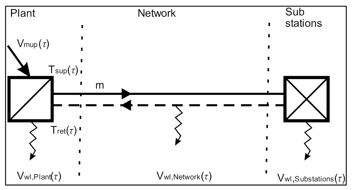
The methodology for determining the amount of water loss in a DHS is presented below. A DHS can be divided into three main parts: heat sources, distribution network, and heating substations (Figure 3). In each part, there are leaks in pipeline systems. In heat sources and substations, leaks occur most frequently in places where pipes are connected and where technological equipment fails. These leaks can be located without specialist equipment as they manifest themselves in the form of a visible water leak. Leakage points in the DHN are far more difficult to locate due to lack of access to the pipes, which are usually below ground or in ducts.

The amount of water leaking from the DHS $V_{wl}$ is the sum of water losses in its individual parts—Equation (7). It should be noted that water losses in substations $V_{wl,Substations}\left(\tau \right)$ concern water leakage through leaks and the amount of water used to supplement internal installations in buildings.

$$V_{wl}\left(\tau \right)=V_{wl,Plant}\left(\tau \right)+V_{wl,Network}\left(\tau \right)+V_{wl,Substations}\left(\tau \right),\frac{{\mathrm{m}}^3}{\mathrm{h}}.$$

(7)

The $V_{wl}$ value can also be defined as the sum of water leaks from individual leaks $V_{wl,i}$ in a DHS—Equation (8). The amount of water discharging through a given leak depends on the water pressure p_i at its location and the water flow resistance $R_{H,i}$—Equation (9). The value of $R_{H,i}$ differs for each leak location and is very difficult to define. However, there are methods to determine the amount of water leaking through a leak in a pipeline [24] by testing the drop in water pressure in a separate and closed section of a DHN. Analysis of the rate of pressure change enables one to estimate the value of resistance of water flow through leaks located in a fragment of the DHN.

The total water stream leaking from the DHS depends on the value and changes in water pressure in the system. Water pressure varies according to the season. Water pressure also varies during the day due to the operation of pumps in heat sources and control valves in substations and due to failures and repairs of heating pipelines.

$$V_{wl}\left(\tau \right)={\displaystyle \sum }_{i=1}^N{V}_{wl,i}\left(\tau \right), \frac{m^3}{h}.$$

(8)

$$V_{wl,i}\left(\tau \right)=f\left(p_i\left(\tau \right),R_{H,i}\right).$$

(9)

Water losses can be determined directly or indirectly. Direct measurement is difficult due to the impossibility of locating all leakage points. It is particularly difficult to locate water leaks in a DHN, which occur directly in the ground or in ducts, and microleaks. Many methods have been developed to locate water leaks [12,13,14,15,16], but they only concern large leaks. For this reason, a method has been adopted to indirectly determine (calculate) the volume of network water losses.

The value of the make-up water flow rate being replenished to the DHS $V_{mup}$ is equal to the sum of the water flow rate leaking through the leaks $V_{wl}$ and the change in its volume resulting from temperature changes in the water flowing through the pipelines $\Delta V_{\Delta \rho }$—Equation (10). Due to minor changes in the temperature of water in the DHN, the changes in the volume of pipelines due to thermal expansion of the material they are made of, i.e., steel, were omitted. Therefore, storage capacity was assumed to be constant and unaffected by changes in water temperature.

$$V_{mup}\left(\tau \right)=V_{wl}\left(\tau \right)+\Delta V_{\Delta \rho }\left(\tau \right),\frac{{\mathrm{m}}^3}{\mathrm{h}}.$$

(10)

The value of the water flowing out of the system (water loss flow rate) was calculated according to Equation (11).

$$V_{wl}\left(\tau \right)=V_{mup}\left(\tau \right)-\Delta V_{\Delta \rho }\left(\tau \right),\frac{{\mathrm{m}}^3}{\mathrm{h}}.$$

(11)

DHSs are characterized by changes in the temperature of water in the DHN, which cause changes in the volume of water and, thus, affect the amount of water supplementing the system. The value of the changes in the volume of water in 1 h can be calculated according to Equations (12) and (13).

$$\Delta V_{\Delta \rho }\left(\tau \right)=\frac{m_w}{\Delta {\rho }_w\left(\tau \right)},\frac{{\mathrm{m}}^3}{\mathrm{h}},$$

(12)

$$\Delta {\rho }_w\left(\tau \right)={\rho }_w\left(T_{\tau ,aver}\right)-{\rho }_w\left(T_{\tau -\Delta \tau ,aver}\right),\frac{\mathrm{kg}}{{\mathrm{m}}^3\mathrm{h}},$$

(13)

where $m_w$ is the water mass in the DHS (kg), $\Delta {\rho }_w\left(\tau \right)$ is the change in average water density value in the DHS within Δτ = 1 h (kg/m³h), and $T_{\tau ,aver}$, $T_{\tau -\Delta \tau ,aver}$ are the average temperature of water in the DHS at time τ and τ – Δτ (°C).

Changes in water temperature result mainly from the method used to regulate the heating system. The value of water temperature depends on current and forecast atmospheric conditions, i.e., on consumer demand for heat. Changes in the average value of water density in a DHS depend on changes in the average value of water temperature $T_{\tau ,aver}$.

Determination of the average value of water density requires knowledge of the average temperature of water in a DHS. Average water temperature can be calculated using programs such as TERMIS [25] and Auditor SCW [26], which require knowledge of actual water parameters in all heating substations and chambers. This information can be obtained from systems monitoring water parameters in the DHS, i.e., the SCADA system. Szczecin, in common with many other DHSs in Poland, does not have an extensive system for monitoring water parameters. Therefore, a simplified model of the DHS was built to carry out the analysis, whose main purpose was to determine the profile of changes in average water temperature during the year.

3.1. Simplified Model of DHN

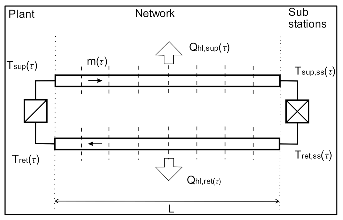
Changes in the density of water in a DHS result from changes in its temperature over time. In order to model this phenomenon, a simplified model of a DHN was made. It makes the following assumptions: the heating system is supplied from a single heat source; heat is supplied to the substitute heating substation by a pipeline of length $L$ and diameter $d_{in}$ (Figure 4). The profile of the water temperature value in the supply and return pipeline is variable in time and depends on changes in the temperature value of water entering the supply $T_{sup}\left(\tau \right)$ and return pipeline $T_{ret,ss}\left(\tau \right)$, heat losses in the supply $Q_{hl,sup}\left(\tau \right)$ and return pipeline $Q_{hl,ret}\left(\tau \right)$, and changes in the value of water flow rate $m\left(\tau \right)$ in the pipeline.

The most important part of the presented DHS model is its simplified DHN model. The DHN model is a substitute pipeline with length $L$ calculated according to Equation (14). The volume of the pipeline is equal to the actual water volume of the DHN. The value of the inner diameter of the pipeline $d_{in}$ should be calculated according to Equation (15). The replacement pipeline’s heat loss is equal to the actual heat loss of the entire DHN.

$$L=\frac{{{\displaystyle \sum }}_{i+1}^I{L}_{CHP1,i}{Q}_{ss,CHP1,i}+{{\displaystyle \sum }}_{j=1}^J{L}_{CHP2,j}{Q}_{ss,CHP2,j}+{{\displaystyle \sum }}_{k=1}^K{L}_{HOB1,k}{Q}_{ss,HOB1,k}+\dots }{{{\displaystyle \sum }}_{i=1}^I{Q}_{ss,CHP1,j}+{{\displaystyle \sum }}_{j=1}^J{Q}_{ss,CHP2,j}+{{\displaystyle \sum }}_{k=1}^K{Q}_{ss,HOB1,k}+\dots }, \mathrm{m}.$$

(14)

$$d_{in}=\sqrt{\frac{2V_n}{\pi L}},\mathrm{m}.$$

(15)

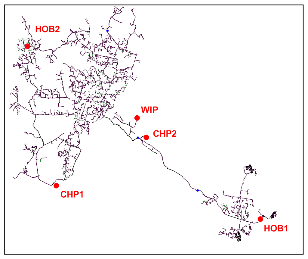
The length and internal diameter of the replacement pipeline may vary during the year due to interruptions in the operation of individual heat sources. The number of working heat sources depends on the current heat demand of consumers and the occurrence of failures and repairs. For the heating system in Szczecin (Figure 1), two scenarios of heat source operation were created: the winter scenario, where all heat sources operate except HOB2, and the summer scenario, where only two heat sources work (HOB1 and WIP). The values of length $L$ and internal diameter $d_{in}$ of the pipeline were determined for the two scenarios of heat source operation—

Table 2. Replacement pipeline parameters for heat source operation scenarios.

Season Scenario	Length of Pipe—Equation (14) L, m	Internal Diameter—Equation (15) din, m
Winter	9722	1.658
Summer	13,931	1.385

.

The temperature of water in a DHS is variable and depends on the heat demand of consumers. Modeling the dynamics of water temperature changes requires the application of an appropriate model of heat transport in a DHN. Models of heat transport through district heating pipelines have been presented in a number of studies [27,28,29,30,31,32,33,34,35]. They mainly concern the phenomena of heat transport for individual pipelines forming part of the entire DHN system.

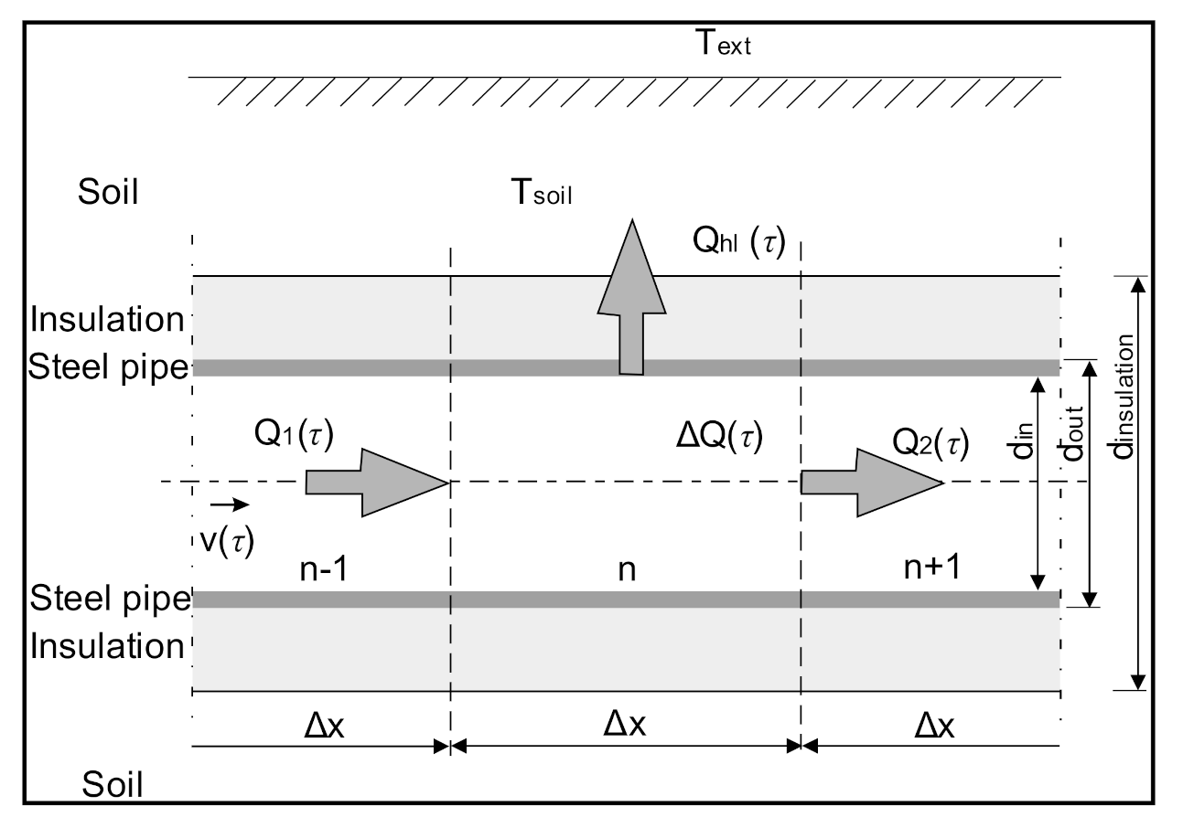
A similar model was used to simulate the dynamics of heat transport in a substitute pipeline (Figure 5). It assumes the discretization of the replacement pipe into split elements of equal length $\Delta x$—element method [29]. The number of N-pipe splits depends on the adopted time step $\Delta \tau$ (1 h) and the value of water velocity $v$ in pipe. The number of pipe splits into balance elements is determined by the relationship in Equation (16).

$$N\left(\tau \right)=trunc\left(\frac{L}{\Delta x\left(\tau \right)}\right)=trunc\left(\frac{L}{v\left(\tau \right)\Delta \tau }\right).$$

(16)

Pipeline splitting enables calculation of the value of water temperature in each element and its change in subsequent moments of time. The value of water temperature in each pipe splitting element is calculated on the basis of heat balance Equation (17). The amount of heat flowing into the element $Q_1\left(\tau \right)$ is equal to the sum of the heat flowing out of the element $Q_2\left(\tau \right)$, heat losses $Q_{hl}\left(\tau \right),$ and energy change inside the element $\Delta Q\left(\tau \right)$.

$$Q_1\left(\tau \right)=Q_2\left(\tau \right)+Q_{hl}\left(\tau \right)+\Delta Q\left(\tau \right), \mathrm{J}.$$

(17)

The following simplifying assumptions were made in the balance sheet equation:

-

Heat conduction between the pipe splitting elements in the direction of the water flow is neglected;

-

Heat conduction in the pipe material in the direction parallel to the direction of water flow is omitted.

The components of the heat balance in Equation (17) can be recorded as follows:

$$Q_1\left(\tau \right)={\rho }_{w}Av\left(\tau \right)c_{w}T\left(x,\tau \right)d\tau ,\mathrm{J}.$$

(18)

$$Q_2\left(\tau \right)={\rho }_{w}Av\left(\tau \right)c_w\left[T\left(x,\tau \right)+\frac{\partial T\left(x,\tau \right)}{\partial x}dx\right]d\tau ,\mathrm{J}.$$

(19)

$$\Delta Q\left(\tau \right)=\left[{\rho }_{w}A{c}_w+{\rho }_{st}{c}_{st}\frac{\pi }{4}\left(d_{out}^2-d_{in}^2\right)\right]\frac{\partial T\left(x,\tau \right)}{\partial \tau }dxd\tau ,\mathrm{J}.$$

(20)

Basing Equations (18)–(20) on the energy balance Equation (17), we obtain its differential form:

$$a_1\frac{\partial T\left(x,\tau \right)}{\partial x}dxd\tau +a_2\frac{\partial T\left(x,\tau \right)}{\partial \tau }dxd\tau +Q_{hl}\left(\tau \right)=0,$$

(21)

where

$$a_1={\rho }_{w}Av\left(\tau \right)c_w,$$

(22)

$$a_2={\rho }_{w}A{c}_w+{\rho }_{st}{c}_{st}\frac{\pi }{4}\left(d_{out}^2-d_{in}^2\right).$$

(23)

The values of the partial derivatives of the temperature function in Equation (21) are approximated by the differential quotients in Equation (24):

$${\left.\frac{\partial T\left(x,\tau \right)}{\partial x}\right|}_n=\frac{\overline{T_n}-\overline{T_{n-1}}}{\Delta x};{\left.\frac{\partial T\left(x,\tau \right)}{\partial \tau }\right|}_n=\frac{T_n-\overline{T_n}}{\Delta \tau }.$$

(24)

Lastly, Equation (20) takes the form in Equation (25), from which the temperature value in a given pipe element $T_n$ is calculated.

$$a_1\left(\overline{T_n}-\overline{T_{n-1}}\right)\Delta \tau +a_2\left(T_n-\overline{T_n}\right)\Delta x+Q_{hl}\left(\tau \right)=0.$$

(25)

Heat losses $Q_{hl}\left(\tau \right)$ are related to the heat flow from water to the ground and external environment. They are modeled according to the relationship in Equation (26). The $R$-value is the heat flow resistance and is the sum of the heat flow resistance through the insulation and the ground [36]. The resistances of heat conduction through the pipe wall and heat transfer at the inner surface of the pipe are negligible and can be ignored. Heat losses are calculated according to Equation (26).

$$Q_{hl}\left(\tau \right)=\frac{\overline{T_n}-T_{soil}}{R}\Delta x\Delta \tau ,\mathrm{J}.$$

(26)

The presented model of the dynamics of heat transport through pipelines is used to determine the value of water temperature $T_n$ in each element of pipe division on the basis of Equation (25). The average value of water temperature in the substitute model of the DHN (Figure 4) is determined according to Equation (27). The values $N_{sup}$, $N_{ret}$ determine the number of splits in the supply and return pipes, while $T_{sup}$, $T_{ret}$ are the water supply and return temperature values in individual pipe split elements.

$$T_{aver}\left(\tau \right)=\frac{\frac{{{\displaystyle \sum }}_{n=1}^{N_{sup}}{T}_{sup,n}}{N_{sup}}+\frac{{{\displaystyle \sum }}_{n=1}^{N_{ret}}{T}_{ret,n}}{N_{ret}}}{2},℃.$$

(27)

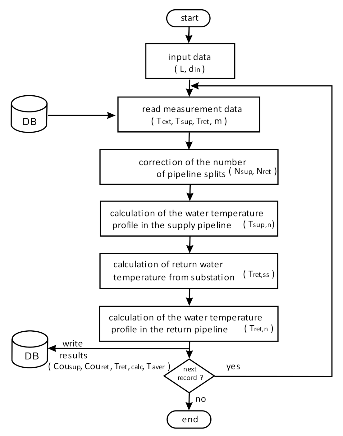
The flowchart of the calculation procedure for average water temperature in DHN is shown in Figure 6.

3.2. Approximation Quality

The condition for a good approximation of the temperature wave flow phenomenon is to ensure that the pipeline is split in such a way that the water flow path at time $\Delta \tau$ is equal to the pipe division length $\Delta x$, i.e., $v\Delta \tau =\Delta x$. An indicator of the quality of approximation of this phenomenon is the dimensionless Courant $\left(Cou\right)$ number [28,29], defined in Equation (28).

$$Cou=\frac{v\Delta \tau }{\Delta x}.$$

(28)

The approximation condition is met with a Courant value equal to (or almost equal to) 1. Due to changes in the speed of water in the pipeline at subsequent moments in time, it is not possible to meet the above condition. For this reason, a modification of the model was introduced consisting in correction of the number of pipeline splits in Equation (16) depending on the current value of velocity of water flowing in the pipeline. In each step of the simulation, the number of splits of the replacement pipeline (supply and return) is adjusted to changes in water flow rate values. With these changes introduced, the value of the Courant number ranged from 0.96 to 0.99 during the whole simulation period. Figure 7a,b show the changes in the Courant value of the supply and return pipeline during the simulation calculation, i.e., for the whole year of 2019 and for the month of May. It should be noted that the value of the Courant number changes slightly with large changes in the water flow rate value, i.e., from about 1000 Mg/h in summer to 6000 Mg/h in winter.

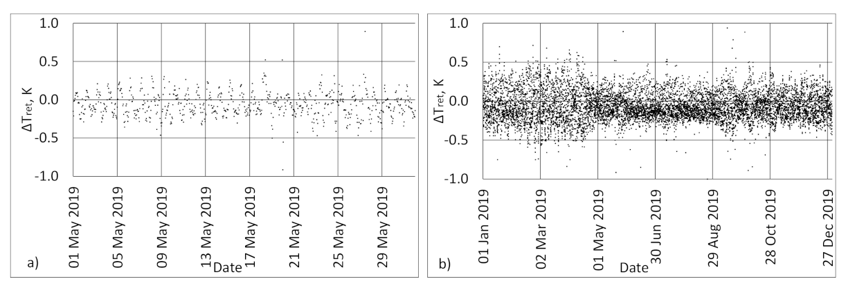
3.3. Verification of the Numerical Model

Verification of the calculations using the described model of DHN was carried out by comparing the results of the calculations $T_{ret,calc}\left(\tau \right)$ with the measured values of temperature $T_{ret}\left(\tau \right)$ of water returning to the heat source. The value of the return water temperature difference was calculated using Equation (29).

$$\Delta T_{ret}\left(\tau \right)=T_{ret}\left(\tau \right)-T_{ret,calc}\left(\tau \right),\mathrm{K}.$$

(29)

Figure 8 presents the results of the numerical model verification performed for the measurement data recorded in 2019 (Figure 8b) and in May 2019 (Figure 8a). The value of the return water temperature difference, $\Delta T_{ret}\left(\tau \right)$, varies from −0.3 K to +0.3 K. The resulting accuracy of the calculation is sufficient for simulation calculations.

3.4. Software Development

The simulation calculations presented in the article were made with a special program written by the author. The presented model of the heating system was implemented in the program. Calculations of water temperature changes were made on the basis of the presented model of heat transport dynamics. The program uses a database (saved in MS Access format) containing the measurement results for the heating system operation parameters. The program was written in the Delphi XE8 Professional C/S environment [37]. The program with its source code is available from [38].

4. Results and Discussion

The results of the analysis of the impact of changes in water density in the DHS on water loss monitoring are presented below.

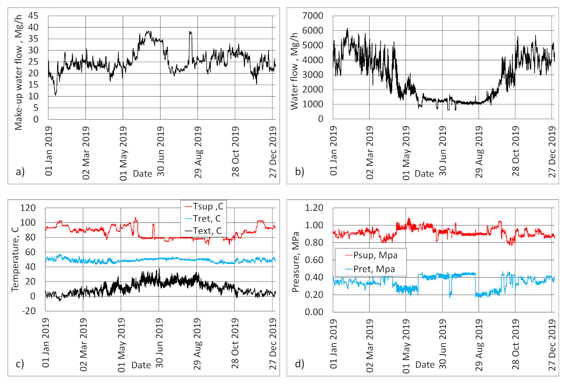
Calculations were made on the basis of processed measurement data according to Equations (1)–(6). The results are presented in Figure 9, showing the profiles of changes in individual parameters during the year.

The value of the make-up water flow rate (Figure 9a) varies from about 20 Mg/h to 30 Mg/h. However, there are periods when the make-up water flow rate significantly exceeds the abovementioned range of variation. This is due to pipeline failure or overhaul. The increase in water make-up flow rate may also derive from the watering of new sections of the network installed to serve new housing developments connecting to the DHN.

Figure 9b shows the changes in total water flow rate in the DHN, varying from 1000 Mg/h in the summer (not heating season) to about 6000 Mg/h in winter (heating season). In the winter, large changes in network water flow rate in the DHS are observed, which are caused by the operation of automatic control systems installed in substations. This often occurs in transition periods when the outside air temperature is between +2 °C and +10 °C.

The values for supply and return water temperature and outside air temperature are shown in Figure 9c. The supply water temperature varies from 78 °C during the summer season to about 100 °C during the winter season. The return water temperature varies from 45 °C to 55 °C. The value of the supply water temperature is due to the way the DHS is regulated and depends on customer heat demand.

The pressure variation profiles of the supply and return water are shown in the diagram (Figure 9d). The water pressure varies in the range 0.8 MPa–1.1 MPa (supply) and 0.20 MPa–0.45 MPa (return). This graph shows guide values, as they only relate to the water pressure values measured in heat sources.

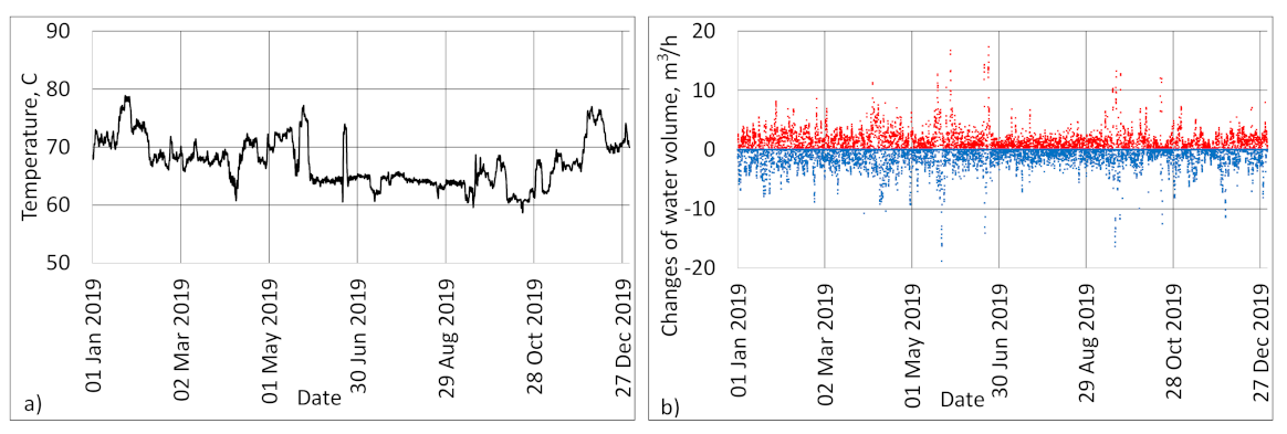
Calculations of the average temperature of water in a DHN were made using the methodology presented in this article and a mathematical model of heat transport dynamics. The calculation results are presented in Figure 10a. In the winter, the amplitude of water temperature changes is from about 67 °C to 78 °C, while, in the summer, the temperature changes are much smaller and range from 60 °C to 65 °C.

The results of calculations of water volume changes resulting from temperature changes are shown in Figure 10b. The increase in water volume is marked with red points and the decrease in water volume is marked with blue points. In the analyzed DHS, whose volume is $V_n=\mathrm{41,974} {\mathrm{m}}^3$, the changes in water volume are from −5 m³/h to about +5 m³/h, sometimes greater.

Figure 11 shows the results of calculations of changes in water volume in the analyzed DHS, during 1 h (black line) for typical days in the winter (Figure 11a) and summer (Figure 11b). The changes in the volume of water in the DHS during the winter are about 2–3 times higher than the changes during the summer, because, in summer, the water temperature is almost constant and does not depend on the outside air temperature value. On the other hand, in winter, the value of the feed water temperature for the DHS is variable and depends on the outside air temperature changes.

The diagrams also show the profiles of changes in the make-up water flow rate supplementing water volume in the DHS (blue line). In winter, the amplitude of changes in the value of the make-up water flow rate is higher than in the summer. The reasons for this are the higher dynamics of water temperature changes in the DHS, increased activity of heating substations and control equipment, and higher water pressure in the DHN.

The red line shows the changes in the value of the water losses from the system through leaks, which were determined using Equation (11). When comparing the profiles of changes in the make-up water flow rate (blue line) and water losses (red line), it should be noted that the changes in the volume of water in a DHS resulting from changes in water temperature have a significant impact on the value of the make-up water flow rate. This can be expressed in terms of PWC (percentage of water volume change) defined as the ratio of water volume changes over an hour to the make-up water flow rate value—Equation (30).

$$PWC\left(\tau \right)=\frac{V_{\Delta \rho }\left(\tau \right)}{V_{mup}\left(\tau \right)}\times 100,\%.$$

(30)

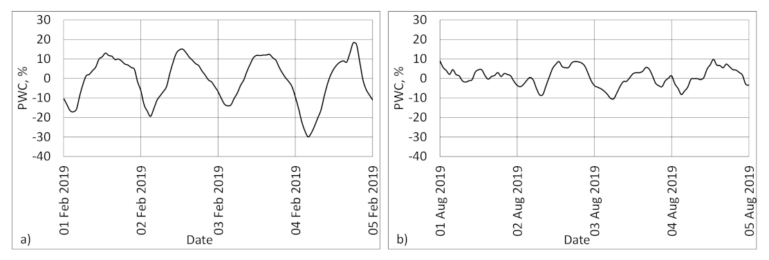
PWC values for the winter vary from approximately −30% to +20% (Figure 12a). For the summer (Figure 12b), the PWC value is smaller, ranging from about −10% to +10%.

Secondary Water Losses

Upgrades to district heating systems have increased their tightness and reduced water losses. When an appropriate level of tightness of the DHS is reached, secondary water losses become more noticeable. They occur when the temperature of water in the DHS rises. Then, an increase in water pressure occurs, causing the safety valves to open, which releases excess water from the system. However, if the water temperature drops, the system needs to be replenished with water. The solution to this problem is to use tanks to store the excess water or to use thermal energy storage [39].

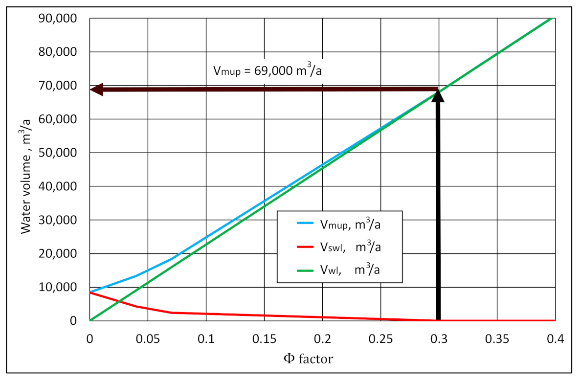
Secondary water loss phenomena for Szczecin DHS are presented in Figure 13. The horizontal axis shows the values of the coefficient of water loss reduction $\left(\Phi \right)$ defined as the ratio of the reduced value of water losses $V_{wl}$ (resulting, e.g., from heating network upgrade) to the current value of water losses $V_{wl,act}$—Equation (31).

$$\Phi =\frac{V_{wl}}{V_{wl,act}}.$$

(31)

The value of $\Phi$ factor varies from: 1.0 (current level of tightness of the heating system) to 0.0 (fully tight heating system).

Figure 11 refers to a DHS that is not equipped with an excess water storage tank or thermal energy storage.

Excess water volume in a DHS appears at $\Phi =0.3$. This corresponds to an annual water exchange ratio of 1.6. It should also be noted that, in the case of a very tight DHS ($\Phi <0.025$), the value of secondary water losses may be higher than water losses due to leaks. For this reason, leakproof systems should be equipped with additional tanks to collect temporary excess water or thermal energy storage tank hooked up directly to the DHS. Where expansion tanks are installed, water stored in the tanks should be used to replenish DHN.

5. Conclusions

The analysis showed that changes in the volume of water in a DHS, caused by changes in water temperature, affect the monitoring of the make-up water flow rate. When the water temperature increases, the value of the make-up water flow rate decreases, and vice versa.

The paper presents the methodology of determining changes in the volume of water in a DHS on the basis of the results of water temperature measurement in heat sources. The model of the dynamics of heat transport through district heating pipelines was used to determine the profiles of water temperature change in the whole DHS and changes in water density.

The change in the volume of water as a result of changes in density in the examined DHS, which has a system water capacity of almost 42,000 m³, is as high as 5 m³ per hour. This represents approximately 20–30% of the make-up water stream of the DHS. For this reason, this phenomenon should not be overlooked when monitoring water losses in DHSs. Measuring systems, based on measuring the make-up water flow rate, should be equipped with modules introducing corrections to the measured values. The methodology presented in the paper can be applied in measuring systems used to monitor water losses and detect emergency states in heating systems. Presented in the paper algorithm could be implemented in DHS performance monitoring systems to increase the accuracy of water loss measurement. This is particularly important for modern fourth- and fifth-generation district heating systems [4,40,41], where low heat transport losses are mandated [42,43].

The percentages of the heat losses of the DHN in Poland during the winter are usually in the range 6–20% and are lower than in the summer, i.e., 17–30% [10]. These percentages of the heat losses strongly depend on the technical structure of the DHS, i.e., fraction (in total length of the piping) of different types of piping placement and insulation technology. Usually, the percentages of heat losses are lower for pre-insulated piping placed directly in the ground and higher for traditionally insulated piping placed in concrete ducts (both are underground piping) and aboveground piping. Given that the value of the heat losses caused by the leakage of pipelines is around 2% to 4% in the total heat transported through the DHN to the heat consumers [9] and given the significant amounts of make-up water entering the system during the year, the problem of system tightness and monitoring of water losses also has a significant impact on the economics of district heating companies. For the vast majority of DHSs in Poland, the annual water exchange ratio is in the range 3–10, meaning that, for large systems, the values of the make-up water volume exceed hundreds of thousands of m³ per year. For example, for the analyzed DHS in Szczecin, the annual heat loss due to leaks is currently around 4% of the total energy transported through DHN, and the annual volume of make-up water is about 790,000 m³/year.

The analysis also showed that, with an increase in the tightness of a DHS caused by, for example, modernization of the heating network and heating substations, secondary losses of water from the DHS may occur. For the DHS in question, they may occur at a system tightness level corresponding to an annual water exchange ratio of 1.6. In order to prevent the occurrence of secondary water losses, an additional tank needs to be built to collect temporary excess water; alternatively, heat storage tanks can be used for this purpose.

Polish heating systems are often so leaky that the above problem does not occur. However, works on sealing the systems are underway, and, in the future, a sufficiently high level of network tightness will be achieved for the phenomenon of secondary losses to become visible during the operation of heating systems.