
Analysis of a Multi-Timescale Framework for the Voltage Control of Active Distribution Grids


Abstract
1. Introduction
2. Impact of DG Installation on the Voltage Profile
- PV: with the controlled reactive power power injection and the controlled active power curtailment.
- ESS: with the controlled active power injection, whereas no reactive power control was considered.
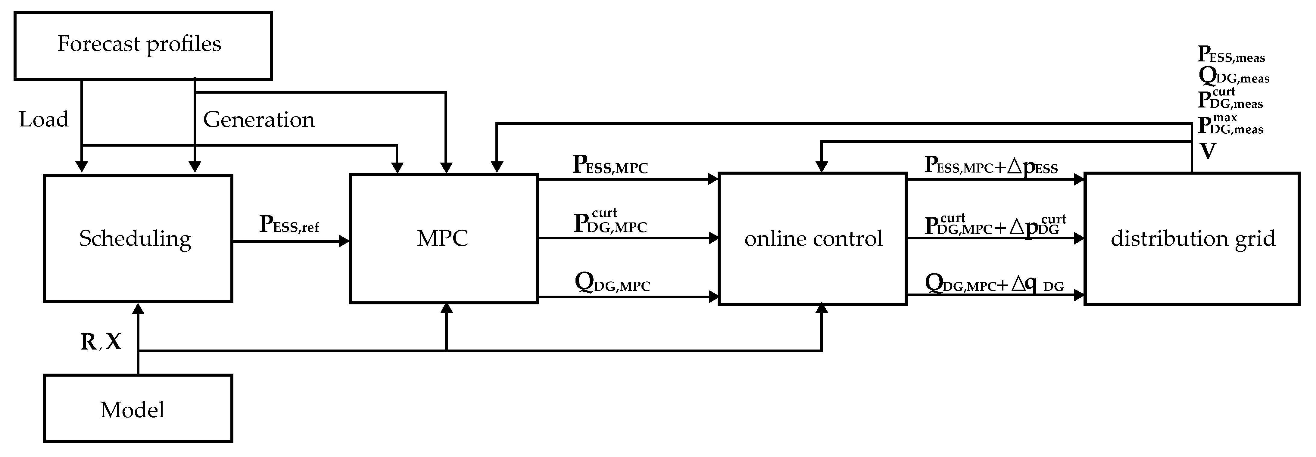
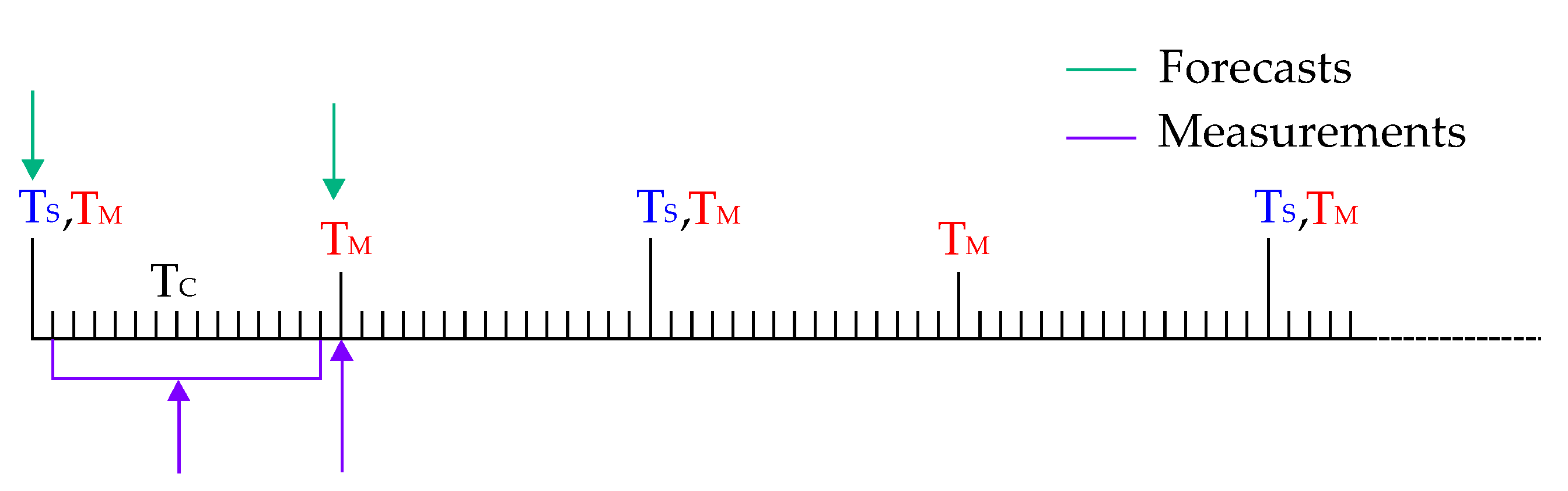
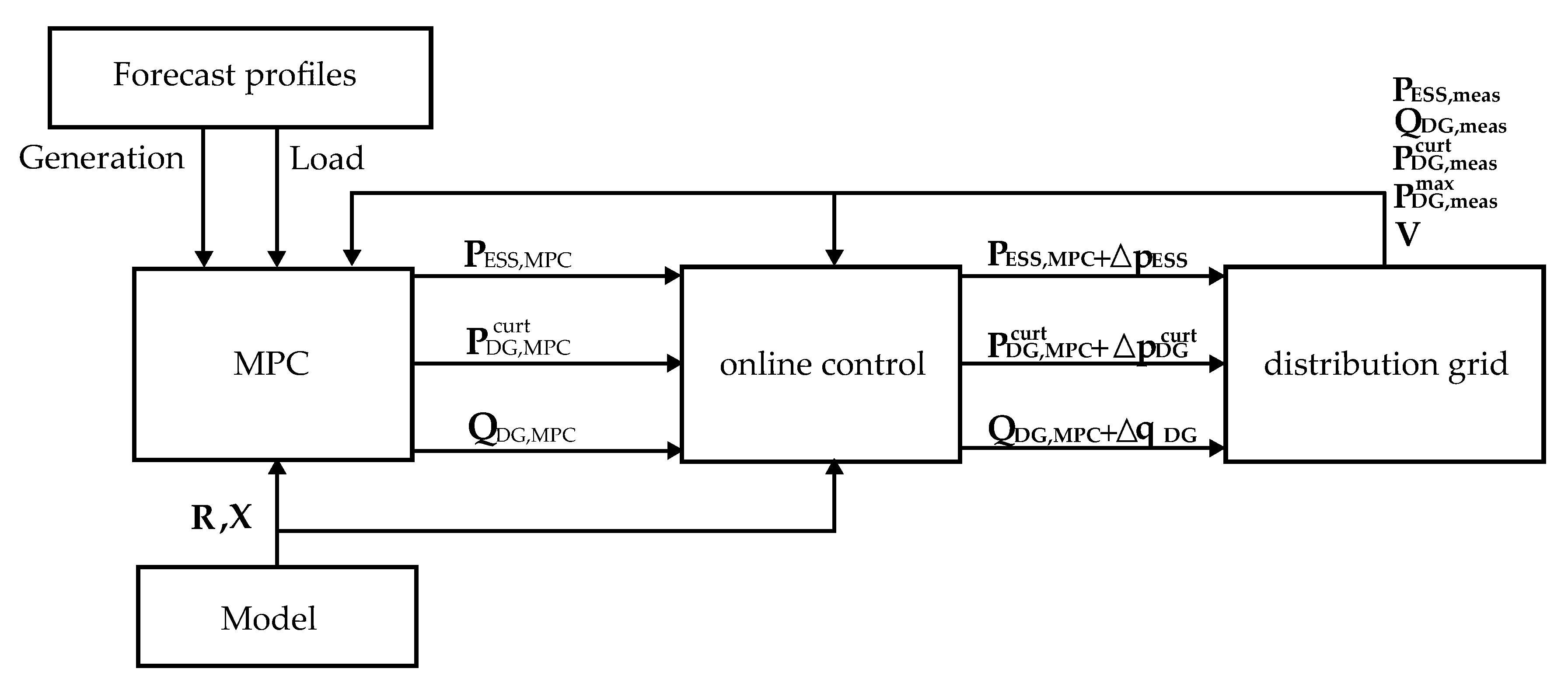
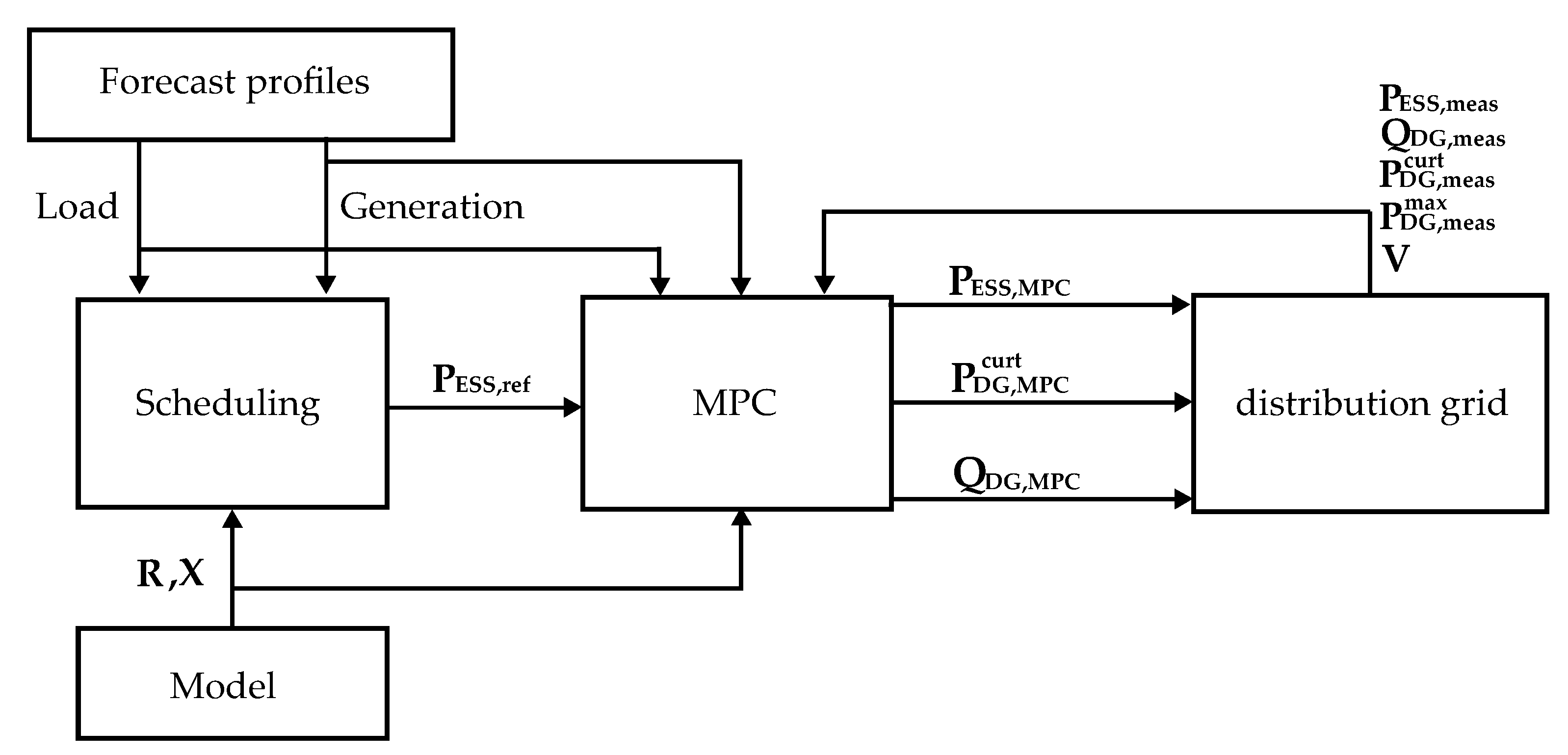
3. Multi-Timescale Framework
3.1. Scheduling of Energy Storage Systems
- is the full vector of voltage magnitudes calculated at iteration
- is the vector of nominal voltage values.
- is the vector of active power set-points assigned to ESSs calculated at iteration .
- are the -dimensional symmetric matrices of weights associated with each variable.
- represents the maximum available DGs’ forecasted active power at the instant .
- represents the active power load forecast at the node where the DGs are installed for the instant .
3.2. Model Predictive Control
- is the vector of active power set-points assigned to the PVs calculated at iteration .
- is the vector of active power set-points assigned to the ESSs calculated at iteration .
- is the vector of reactive power set-points assigned to the PVs calculated at iteration .
- is the SoC calculated at time-step .
- are the N-dimensional symmetric weighting matrices linked to the variables , , and , respectively.
3.3. Online Feedback Control for Fast Dynamics
4. Simulation Setup
4.1. Simulation Description
- Test 1, framework without the scheduler: In this test, the full framework was compared with a case where the scheduler was removed from the framework, to demonstrate that a framework consisting only of the MPC and online control can lead the voltage close to the nominal value, but does not optimally control the SoC of the ESSs.
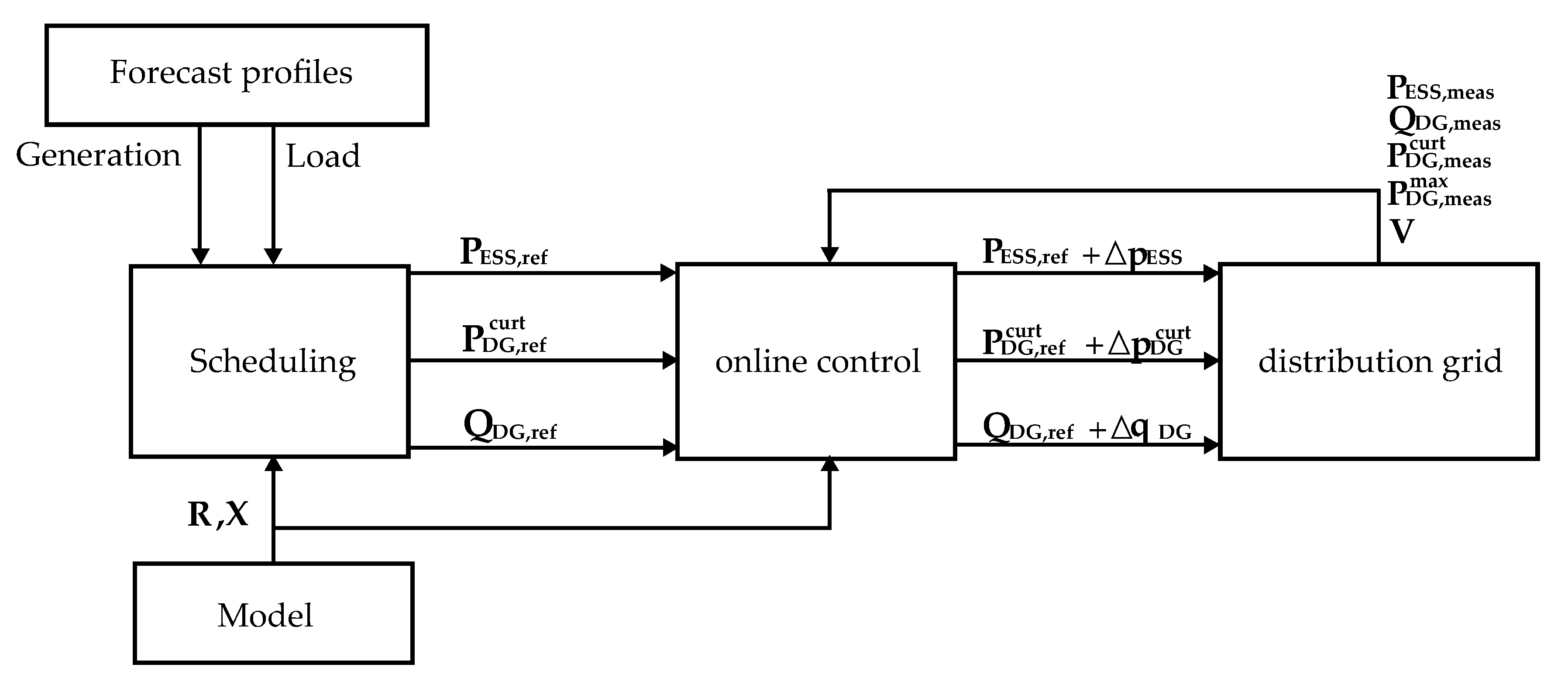
- Test 2, framework without the MPC: In this test, the full framework was compared with a case where the MPC was removed, to show the importance of the MPC in creating set-points for PVs and ESSs that are able to compensate for the forecast errors in the scheduling. In this case, the scheduler calculates the reference values for the PVs and ESSs, which are used directly in the online feedback control.
- Test 3, framework without the online control: In this test, the online feedback control was removed. The purpose of this test was to demonstrate the capability of the online control to solve voltage violations due to rapid variations of the load and generation profiles. Thus, the full framework was compared with a structure without the online control. For this test, the MPC transmits the power set-points every time-step without being modified by the low-level control.
- Loading (W): This indicator was applied in Test 1 and Test 2 and calculated the total loading index as the sum of the power flowing though the branches () calculated for the full day:where is the number of data points obtained from the simulation of the whole day and the number of branches of the grid.
- Voltage variation (%): This indicator was used in Test 1 and Test 2 and calculated the sum of the percentage voltage variation on all nodes for the whole day, compared to the nominal value.
- : This indicator verified the achievement of the condition on the SoC, and it was applied in Test 1 and Test 2. The indicator is defined as:
- Voltage outside the limits (%): This was the only indicator used in Test 3 and calculated the percentage of time that the voltage remained outside the two limits compared to the full day, calculated as:where is the number of simulated data points where the voltage violates the limits.
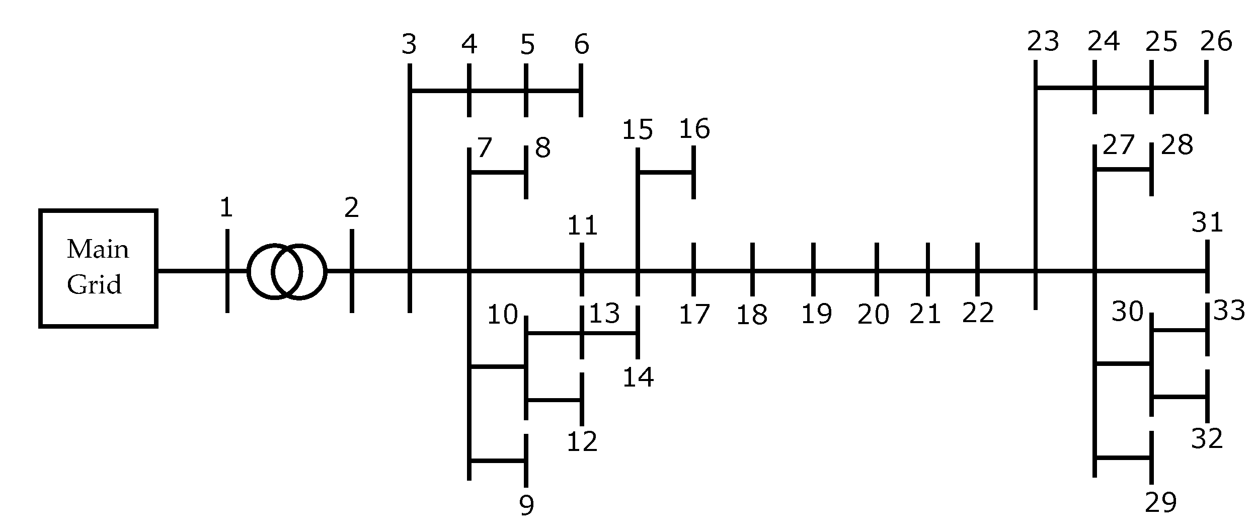
4.2. Grid Data
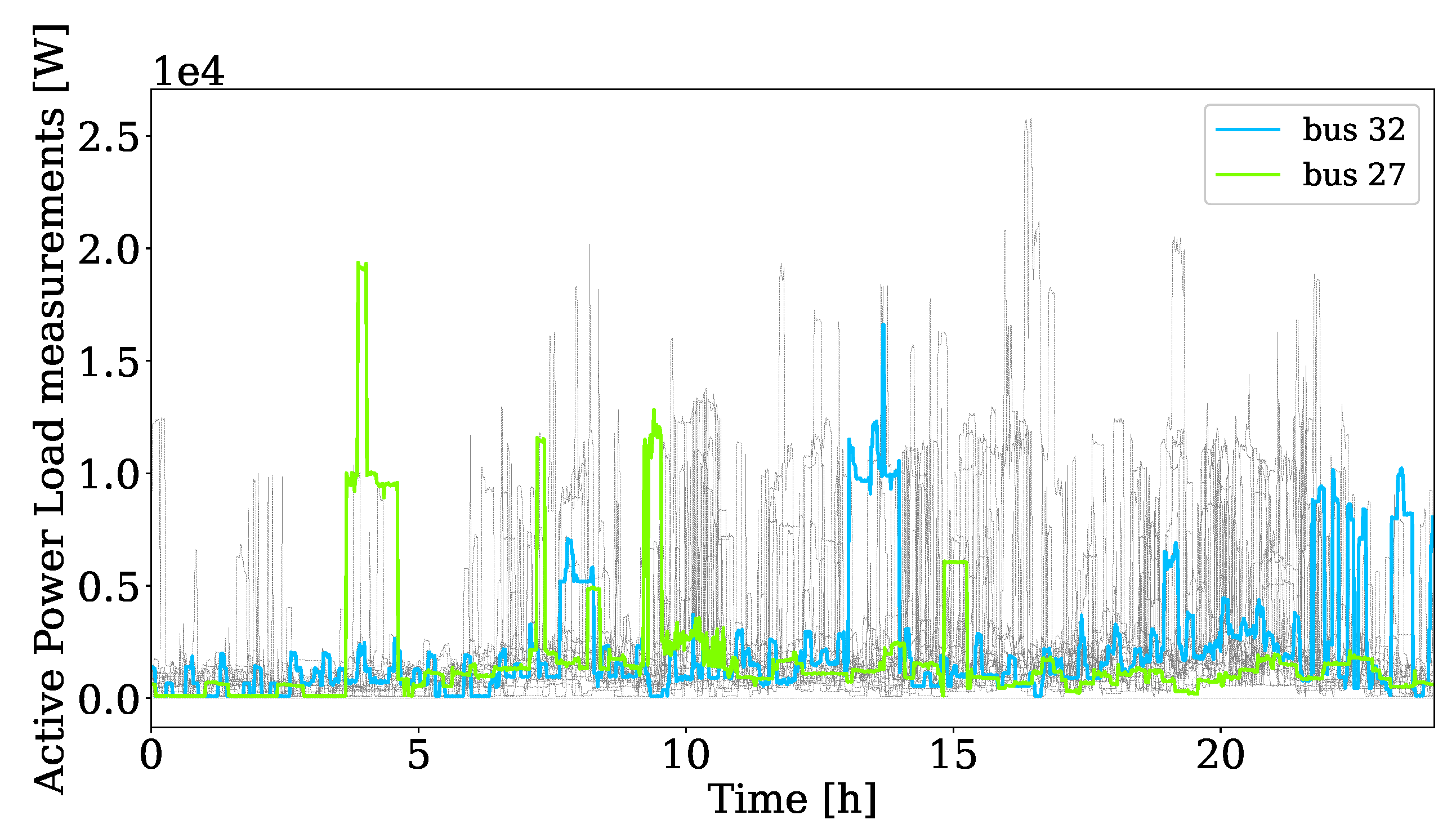
4.3. Load Data
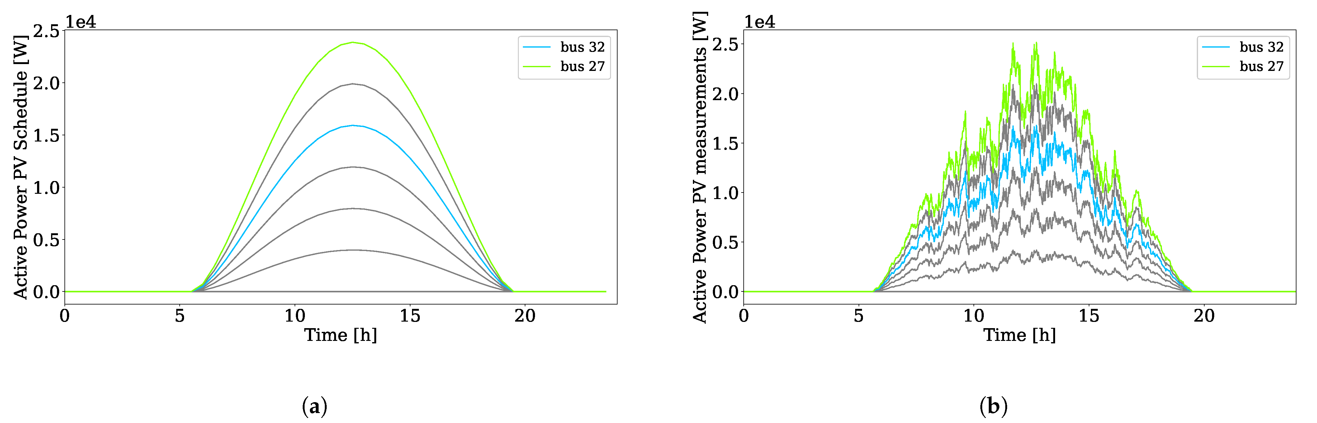
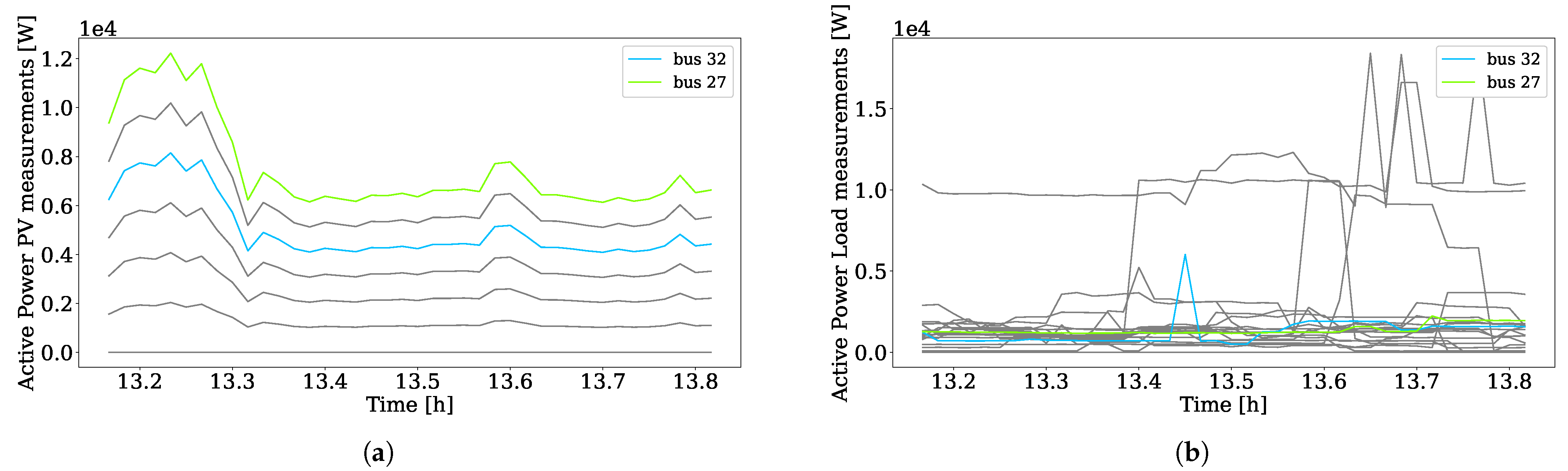
4.4. Generation Data
4.5. Data for Test 3
5. Simulation Results
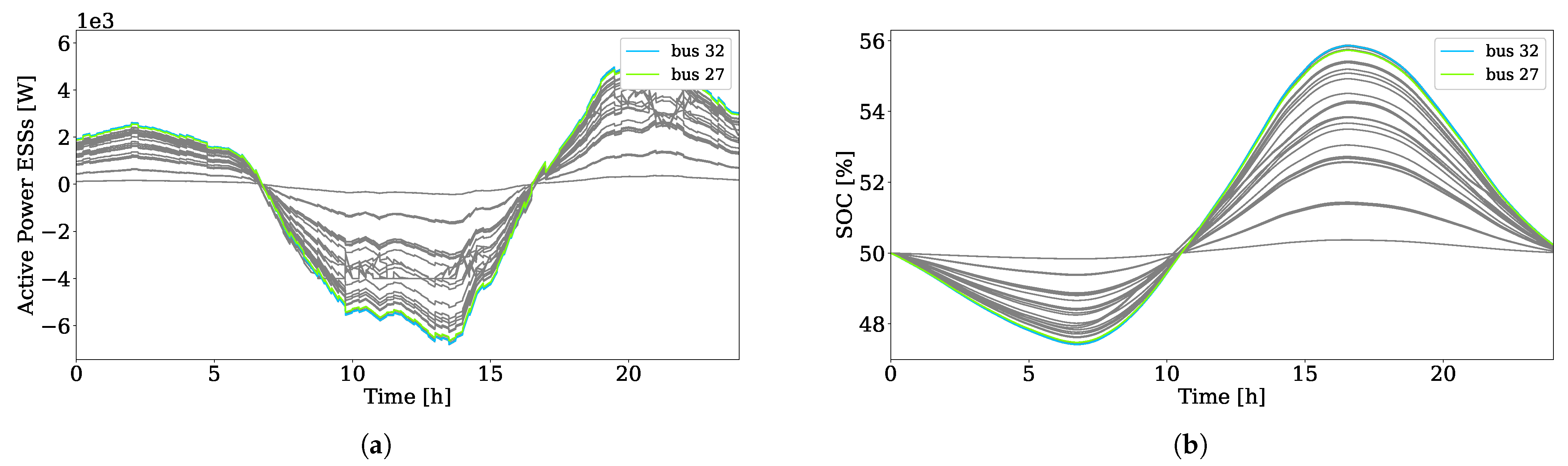
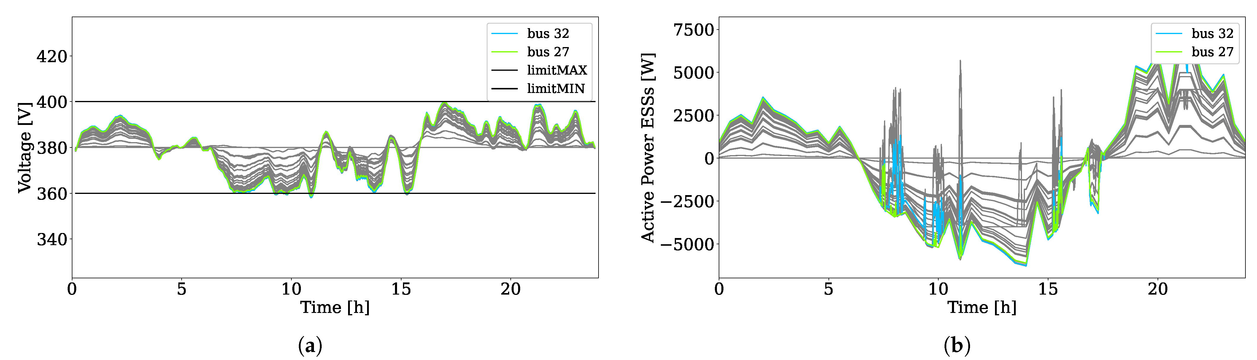
5.1. Complete Multi-Timescale Framework
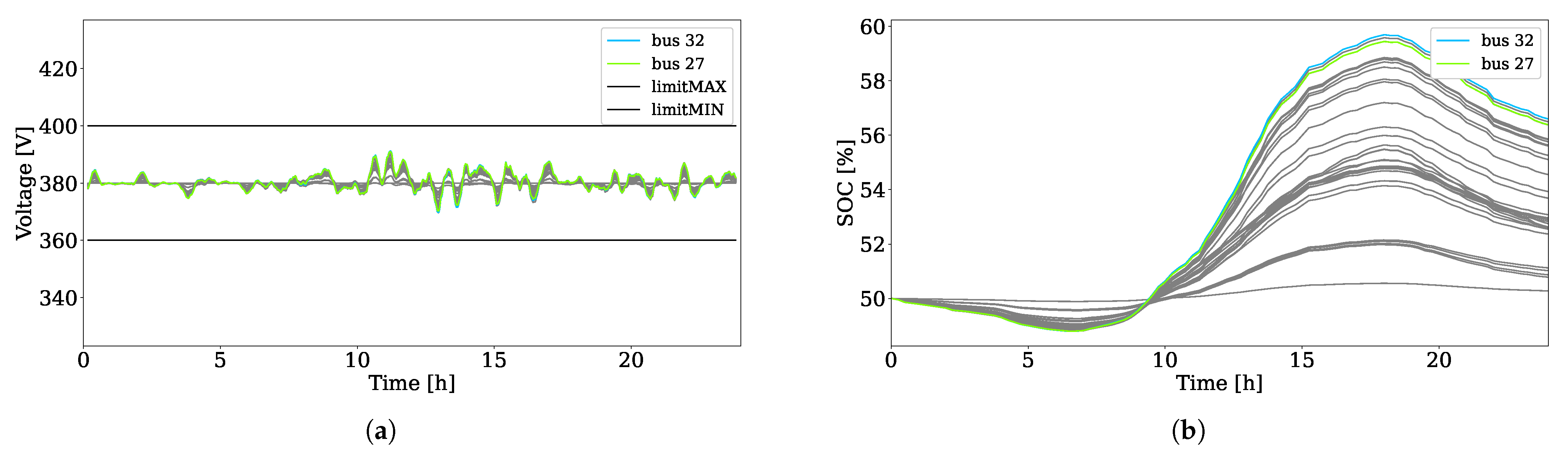
5.2. Test 1: Framework without the Scheduler
- is the -dimensional symmetric weighting matrix linked to the variable .
- The results of the MPC optimization are the set-points values , , and , which are defined as the sum of the last measured value and the result of the first iteration of the MPC.
5.3. Test 2: Framework without the MPC
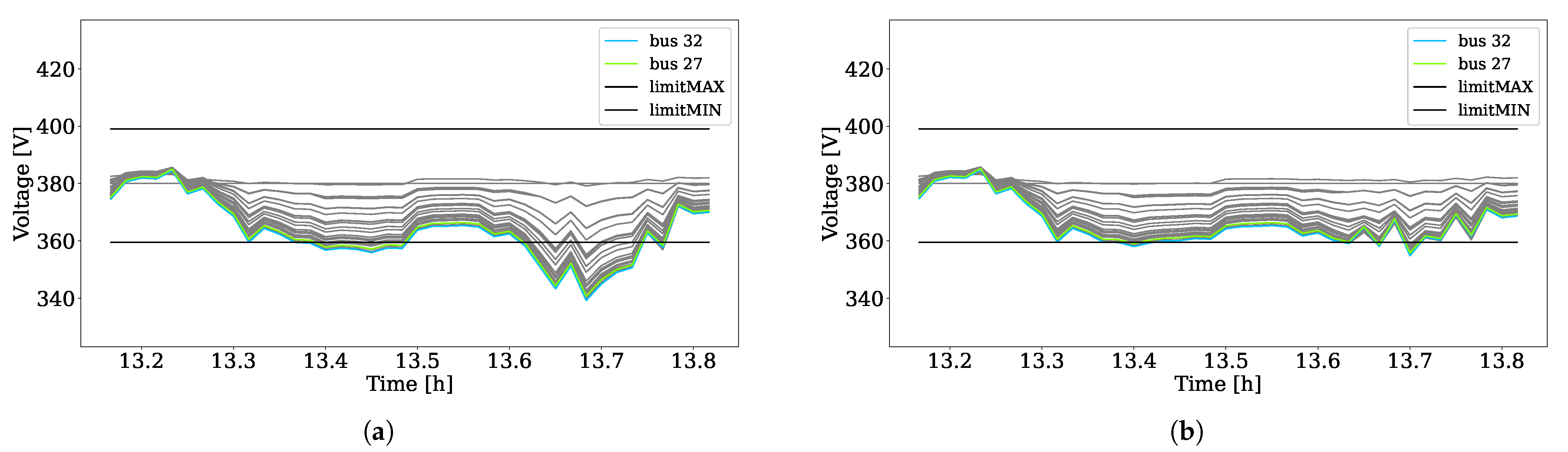
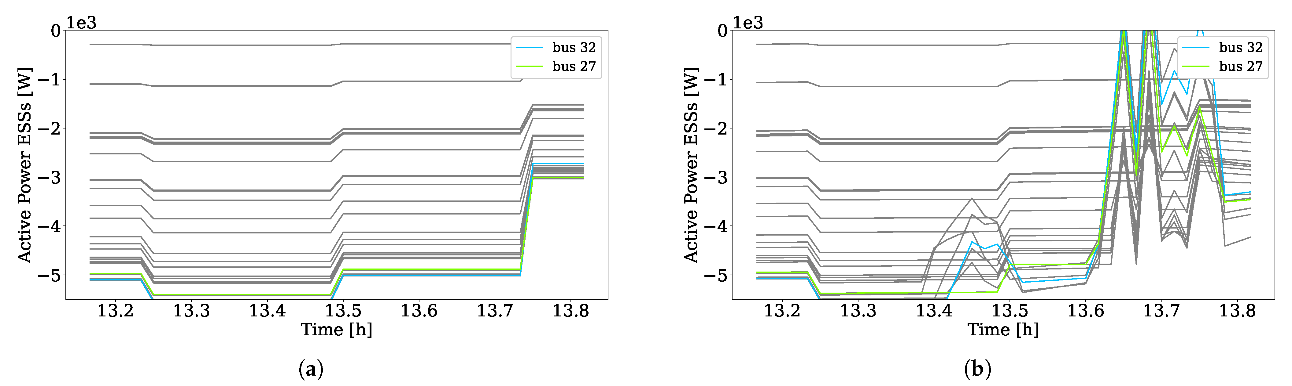
5.4. Test 3: Framework without the Online Control
6. Conclusions
Author Contributions
Funding
Institutional Review Board Statement
Informed Consent Statement
Acknowledgments
Conflicts of Interest
References
- Voltage Characteristics of Electricity Supplied by Public Electricity Networks. EN 50160, 2010.
- IEEE. IEEE Standard for Interconnection and Interoperability of Distributed Energy Resources with Associated Electric Power Systems Interfaces. In IEEE Std 1547-2018 (Revision of IEEE Std 1547-2003); IEEE: Piscatway, NJ, USA, 2018; pp. 1–138. [Google Scholar]
- Generators connected to the low-voltage distribution network: Technical requirements for the connection to and parallel operation with low-voltage distribution networks. VDE Ref. VDE-AR-N 4105, 2008.
- Zarrilli, D.; Giannitrapani, A.; Paoletti, S.; Vicino, A. Energy storage operation for voltage control in distribution networks: A receding horizon approach. IEEE Trans. Control Syst. Technol. 2017, 26, 599–609. [Google Scholar] [CrossRef]
- Von Appen, J.; Braun, M.; Stetz, T.; Diwold, K.; Geibel, D. Time in the sun: The challenge of high PV penetration in the German electric grid. IEEE Power Energy Mag. 2013, 11, 55–64. [Google Scholar] [CrossRef]
- Hashemi, S.; Østergaard, J. Methods and strategies for overvoltage prevention in low voltage distribution systems with PV. IET Renew. Power Gener. 2016, 11, 205–214. [Google Scholar] [CrossRef]
- Collier, S.E. Ten steps to a smarter grid. IEEE Ind. Appl. Mag. 2010, 16, 62–68. [Google Scholar] [CrossRef]
- Strezoski, L.; Stefani, I.; Brbaklic, B. Active Management of Distribution Systems with High Penetration of Distributed Energy Resources. In Proceedings of the IEEE EUROCON 2019-18th International Conference on Smart Technologies, Novi Sad, Serbia, 1–4 July 2019; pp. 1–5. [Google Scholar]
- Zidar, M.; Georgilakis, P.S.; Hatziargyriou, N.D.; Capuder, T.; Škrlec, D. Review of energy storage allocation in power distribution networks: Applications, methods and future research. IET Gener. Transm. Distrib. 2016, 10, 645–652. [Google Scholar] [CrossRef]
- Hesse, H.C.; Schimpe, M.; Kucevic, D.; Jossen, A. Lithium-ion battery storage for the grid—A review of stationary battery storage system design tailored for applications in modern power grids. Energies 2017, 10, 2107. [Google Scholar] [CrossRef]
- Mokhtari, G.; Nourbakhsh, G.; Anvari-Moghadam, A.; Ghasemi, N.; Saberian, A. Optimal cooperative management of energy storage systems to deal with over-and under-voltages. Energies 2017, 10, 293. [Google Scholar] [CrossRef]
- Von Appen, J.; Stetz, T.; Braun, M.; Schmiegel, A. Local voltage control strategies for PV storage systems in distribution grids. IEEE Trans. Smart Grid 2014, 5, 1002–1009. [Google Scholar] [CrossRef]
- Park, S.; Park, W.K. CES peak demand shaving with energy storage system. In Proceedings of the 2017 International Conference on Information and Communication Technology Convergence (ICTC), Jeju Island, South Korea, 18–20 October 2017; pp. 1124–1126. [Google Scholar]
- Bayer, B.; Matschoss, P.; Thomas, H.; Marian, A. The German experience with integrating photovoltaic systems into the low-voltage grids. Renew. Energy 2018, 119, 129–141. [Google Scholar] [CrossRef]
- Sossan, F.; Namor, E.; Cherkaoui, R.; Paolone, M. Achieving the dispatchability of distribution feeders through prosumers data driven forecasting and model predictive control of electrochemical storage. IEEE Trans. Sustain. Energy 2016, 7, 1762–1777. [Google Scholar] [CrossRef]
- Gupta, R.K.; Sossan, F.; Paolone, M. Grid-aware distributed model predictive control of heterogeneous resources in a distribution network: Theory and experimental validation. In IEEE Transactions on Energy Conversion; IEEE: Piscatway, NJ, USA, 2020. [Google Scholar]
- Malekpour, A.R.; Annaswamy, A.M.; Shah, J. Hierarchical Hybrid Architecture for Volt/Var Control of Power Distribution Grids. IEEE Trans. Power Syst. 2019, 35, 854–863. [Google Scholar] [CrossRef]
- Faraji, J.; Abazari, A.; Babaei, M.; Muyeen, S.; Benbouzid, M. Day-Ahead Optimization of Prosumer Considering Battery Depreciation and Weather Prediction for Renewable Energy Sources. Appl. Sci. 2020, 10, 2774. [Google Scholar] [CrossRef]
- Babaei, M.; Abazari, A.; Muyeen, S. Coordination between Demand Response Programming and Learning-Based FOPID Controller for Alleviation of Frequency Excursion of Hybrid Microgrid. Energies 2020, 13, 442. [Google Scholar] [CrossRef]
- Antoniadou-Plytaria, K.E.; Kouveliotis-Lysikatos, I.N.; Georgilakis, P.S.; Hatziargyriou, N.D. Distributed and decentralized voltage control of smart distribution networks: Models, methods, and future research. IEEE Trans. Smart Grid 2017, 8, 2999–3008. [Google Scholar] [CrossRef]
- Bolognani, S.; Carli, R.; Cavraro, G.; Zampieri, S. On the Need for Communication for Voltage Regulation of Power Distribution Grids. IEEE Trans. Control Netw. Syst. 2019, 6, 1111–1123. [Google Scholar] [CrossRef]
- Bernstein, A.; Dall’Anese, E. Real-time feedback-based optimization of distribution grids: A unified approach. IEEE Trans. Control Netw. Syst. 2019, 6, 1197–1209. [Google Scholar] [CrossRef]
- De Din, E.; Pau, M.; Ponci, F.; Monti, A. A Coordinated Voltage Control for Overvoltage Mitigation in LV Distribution Grids. Energies 2020, 13, 2007. [Google Scholar] [CrossRef]
- Gupta, R.; Sossan, F.; Scolari, E.; Namor, E.; Fabietti, L.; Jones, C.; Paolone, M. An admm-based coordination and control strategy for pv and storage to dispatch stochastic prosumers: Theory and experimental validation. In Proceedings of the 2018 Power Systems Computation Conference (PSCC), Dublin, Ireland, 11–15 June 2018; pp. 1–7. [Google Scholar]
- Li, P.; Ji, J.; Ji, H.; Jian, J.; Ding, F.; Wu, J.; Wang, C. MPC-based local voltage control strategy of DGs in active distribution networks. IEEE Transact. Sustain. Energy 2020, 11, 2911–2921. [Google Scholar] [CrossRef]
- Ulbig, A.; Arnold, M.; Chatzivasileiadis, S.; Andersson, G. Framework for multiple timescale cascaded MPC application in power systems. IFAC Proc. Vol. 2011, 44, 10472–10480. [Google Scholar] [CrossRef]
- Fard, A.Y.; Shadmand, M.B. Multitimescale Three-Tiered Voltage Control Framework for Dispersed Smart Inverters at the Grid Edge. IEEE Trans. Ind. Appl. 2020, 57, 824–834. [Google Scholar] [CrossRef]
- Martins, V.F.; Borges, C.L. Active distribution network integrated planning incorporating distributed generation and load response uncertainties. IEEE Trans. Power Syst. 2011, 26, 2164–2172. [Google Scholar] [CrossRef]
- Daghi, M.; Sedghi, M.; Aliakbar-Golkar, M. Optimal battery planning in grid connected distributed generation systems considering different technologies. In Proceedings of the 2015 20th Conference on Electrical Power Distribution Networks Conference (EPDC), Zahedan, Iran, 28–29 April 2015; pp. 138–142. [Google Scholar]
- Farivar, M.; Chen, L.; Low, S. Equilibrium and dynamics of local voltage control in distribution systems. In Proceedings of the 52nd IEEE Conference on Decision and Control, Firenze, Italy, 10–13 December 2013; pp. 4329–4334. [Google Scholar]
- Ouammi, A.; Dagdougui, H.; Dessaint, L.; Sacile, R. Coordinated model predictive-based power flows control in a cooperative network of smart microgrids. IEEE Trans. Smart Grid 2015, 6, 2233–2244. [Google Scholar] [CrossRef]
- Singh, M.; Kar, I.; Kumar, P. Influence of EV on grid power quality and optimizing the charging schedule to mitigate voltage imbalance and reduce power loss. In Proceedings of the 14th International Power Electronics and Motion Control Conference EPE-PEMC, Ohrid, North Macedonia, 6–8 October 2010; pp. T2–196. [Google Scholar]
- Liserre, M.; Buticchi, G.; Andresen, M.; De Carne, G.; Costa, L.F.; Zou, Z.X. The smart transformer: Impact on the electric grid and technology challenges. IEEE Ind. Electron. Mag. 2016, 10, 46–58. [Google Scholar] [CrossRef]
- Olivella-Rosell, P.; Lloret-Gallego, P.; Munné-Collado, Í.; Villafafila-Robles, R.; Sumper, A.; Ottessen, S.Ø; Rajasekharan, J.; Bremdal, B.A. Local flexibility market design for aggregators providing multiple flexibility services at distribution network level. Energies 2018, 11, 822. [Google Scholar] [CrossRef]
- Guo, Y.; Wu, Q.; Gao, H.; Chen, X.; Østergaard, J.; Xin, H. MPC-based coordinated voltage regulation for distribution networks with distributed generation and energy storage system. IEEE Trans. Sustain. Energy 2018, 10, 1731–1739. [Google Scholar] [CrossRef]
- Notarnicola, I.; Notarstefano, G. Constraint-coupled distributed optimization: A relaxation and duality approach. IEEE Trans. Control Netw. Syst. 2019, 7, 483–492. [Google Scholar] [CrossRef]
- Pau, M.; Patti, E.; Barbierato, L.; Estebsari, A.; Pons, E.; Ponci, F.; Monti, A. Design and accuracy analysis of multilevel state estimation based on smart metering infrastructure. IEEE Trans. Instrum. Meas. 2019, 68, 4300–4312. [Google Scholar] [CrossRef]
- Bolognani, S.; Carli, R.; Cavraro, G.; Zampieri, S. Distributed reactive power feedback control for voltage regulation and loss minimization. IEEE Trans. Autom. Control 2015, 60, 966–981. [Google Scholar] [CrossRef]
- PYPOWER. Available online: https://pypi.org/project/PYPOWER/ (accessed on 31 March 2021).
- Hashemi, S.; Østergaard, J. Efficient control of energy storage for increasing the PV hosting capacity of LV grids. IEEE Trans. Smart Grid 2016, 9, 2295–2303. [Google Scholar] [CrossRef]
- Flexible Smart Metering for Multiple Energy Vectors with Active Prosumers. Available online: https://ec.europa.eu/inea/en/horizon-2020/projects/h2020-energy/grids/flexmeter (accessed on 31 March 2021).
- Pau, M.; Angioni, A.; Ponci, F.; Monti, A. A Tool for the Generation of Realistic PV Profiles for Distribution Grid Simulations. In Proceedings of the 2019 International Conference on Clean Electrical Power (ICCEP), Puglia, Italy, 2–4 July 2019; pp. 193–198. [Google Scholar]


| Start | End | P Unit Resistance | Per Unit Reactance | Start | End | P Unit Resistance | Per Unit Reactance |
|---|---|---|---|---|---|---|---|
| 1 | 2 | 4.00 | 3.17 | 17 | 18 | 6.60 | 2.50 |
| 2 | 3 | 1.08 | 4.10 | 18 | 19 | 5.30 | 2.00 |
| 3 | 4 | 4.30 | 1.60 | 19 | 20 | 8.10 | 3.10 |
| 4 | 5 | 8.70 | 3.30 | 20 | 21 | 3.40 | 1.20 |
| 5 | 6 | 9.30 | 3.50 | 21 | 22 | 2.60 | 9.00 |
| 3 | 7 | 1.35 | 5.10 | 22 | 23 | 4.50 | 1.70 |
| 7 | 8 | 3.00 | 1.00 | 23 | 24 | 4.20 | 1.60 |
| 7 | 9 | 6.80 | 2.50 | 24 | 25 | 8.70 | 3.30 |
| 7 | 10 | 9.80 | 3.70 | 25 | 26 | 9.30 | 3.50 |
| 7 | 11 | 7.10 | 2.60 | 23 | 27 | 1.35 | 5.10 |
| 10 | 12 | 9.80 | 3.70 | 27 | 28 | 3.00 | 1.00 |
| 10 | 13 | 7.20 | 2.70 | 27 | 29 | 6.80 | 2.50 |
| 13 | 14 | 4.10 | 1.50 | 27 | 30 | 9.80 | 3.70 |
| 11 | 15 | 9.10 | 3.40 | 27 | 31 | 7.10 | 2.60 |
| 15 | 16 | 8.00 | 3.00 | 30 | 32 | 9.80 | 3.70 |
| 15 | 17 | 3.40 | 1.30 | 30 | 33 | 7.20 | 2.70 |
| Node | 1 | 2 | 3 | 4 | 5 | 6 | 7 | 8 | 9 | 10 | 11 | 12 | 13 | 14 | 15 | 16 | 17 | 18 |
| Customers | 0 | 2 | 1 | 1 | 1 | 2 | 6 | 1 | 3 | 3 | 2 | 4 | 2 | 1 | 2 | 3 | 1 | 2 |
| Node | 19 | 20 | 21 | 22 | 23 | 24 | 25 | 26 | 27 | 28 | 29 | 30 | 31 | 32 | 33 | |||
| Customers | 5 | 2 | 4 | 4 | 5 | 1 | 1 | 2 | 6 | 1 | 3 | 3 | 2 | 4 | 2 |
| Indicators | Uncontrolled | Full Controlled | Test 1 | Test 2 |
|---|---|---|---|---|
| Loading (W) | 3922 | 830 | 340 | 1067 |
| Voltage variation (%) | 10.9 | 4.1 | 2.5 | 6.7 |
| 0.0 | 5.2 | 116 | 7.3 |
| Indicators | With Online Control | Without Online Control |
|---|---|---|
| Voltage outside the limits (%) | 0.45 | 1.5 |
Publisher’s Note: MDPI stays neutral with regard to jurisdictional claims in published maps and institutional affiliations. |
© 2021 by the authors. Licensee MDPI, Basel, Switzerland. This article is an open access article distributed under the terms and conditions of the Creative Commons Attribution (CC BY) license (https://creativecommons.org/licenses/by/4.0/).
Share and Cite
De Din, E.; Bigalke, F.; Pau, M.; Ponci, F.; Monti, A. Analysis of a Multi-Timescale Framework for the Voltage Control of Active Distribution Grids. Energies 2021, 14, 1965. https://doi.org/10.3390/en14071965
De Din E, Bigalke F, Pau M, Ponci F, Monti A. Analysis of a Multi-Timescale Framework for the Voltage Control of Active Distribution Grids. Energies. 2021; 14(7):1965. https://doi.org/10.3390/en14071965
Chicago/Turabian StyleDe Din, Edoardo, Fabian Bigalke, Marco Pau, Ferdinanda Ponci, and Antonello Monti. 2021. "Analysis of a Multi-Timescale Framework for the Voltage Control of Active Distribution Grids" Energies 14, no. 7: 1965. https://doi.org/10.3390/en14071965
APA StyleDe Din, E., Bigalke, F., Pau, M., Ponci, F., & Monti, A. (2021). Analysis of a Multi-Timescale Framework for the Voltage Control of Active Distribution Grids. Energies, 14(7), 1965. https://doi.org/10.3390/en14071965