
Flexible Transmission Network Expansion Planning Based on DQN Algorithm

 ,
,  ,
, 
Abstract
1. Introduction
- A TNEP model including the indexes of the economy, reliability, and flexibility is proposed to ensure the comprehensiveness of the scheme. Moreover, the proposed model considers N-1 security constraints, N-k faults, and the fault severity of the equipment.
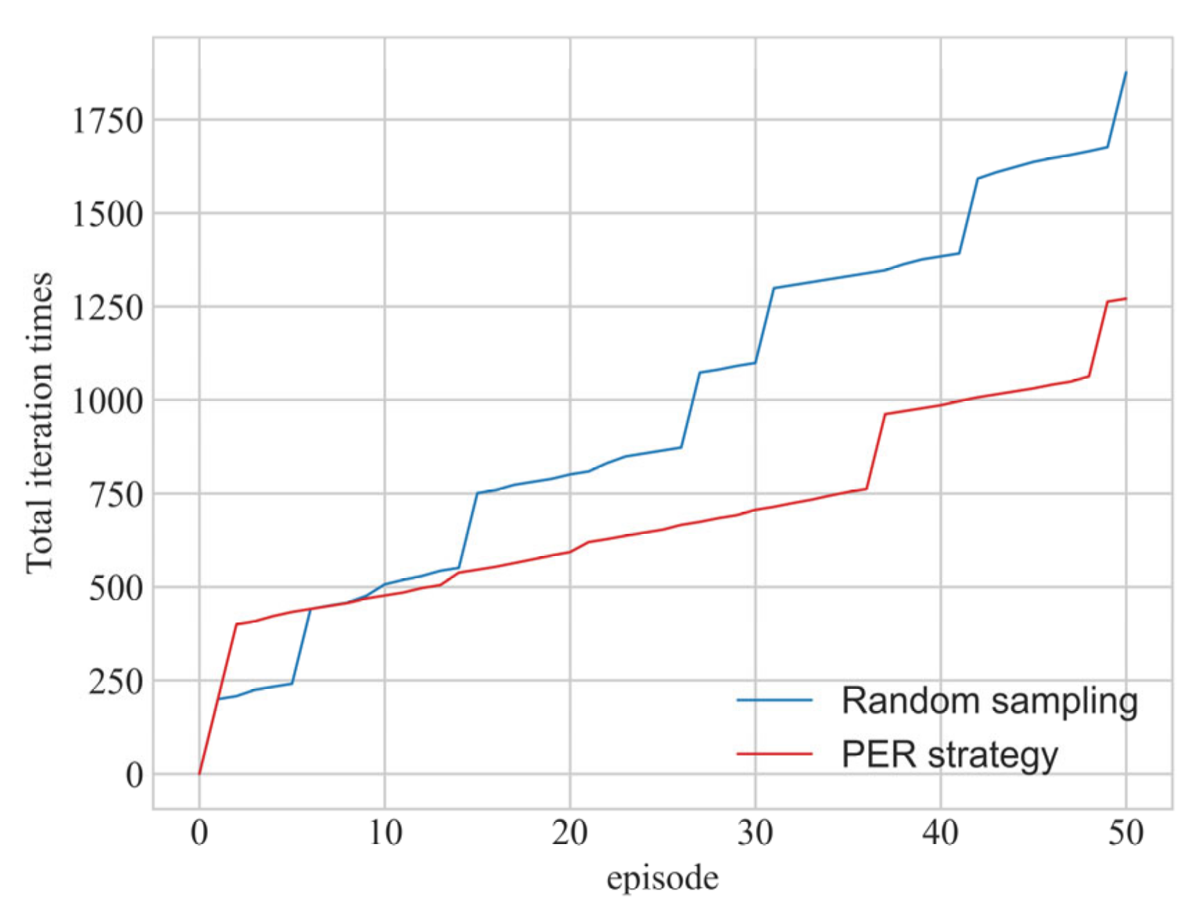
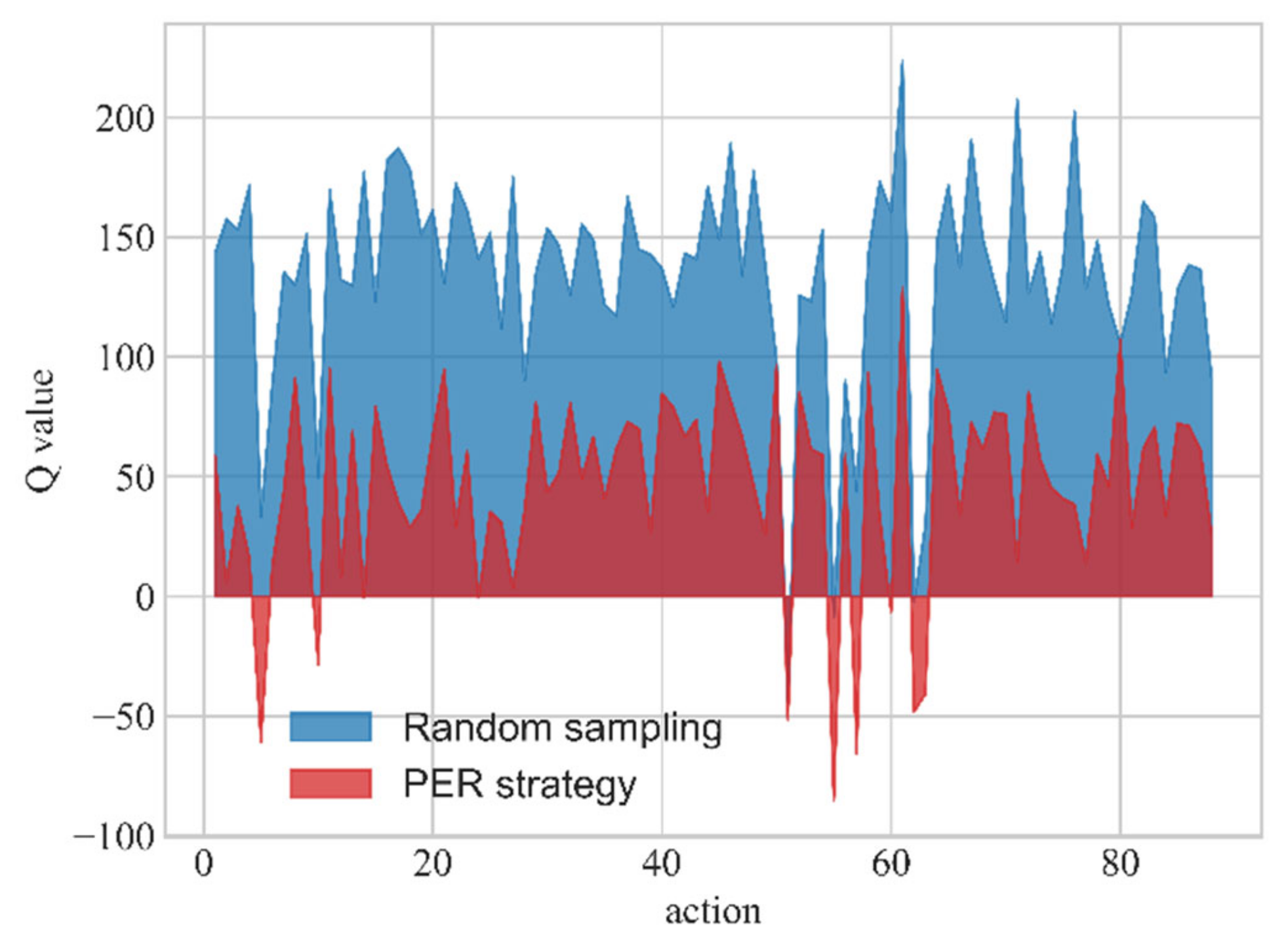
- We introduce a DQN algorithm for the first time in the solution of the TNEP problem and add prioritized experience replay (PER) strategy [35] to the traditional DQN algorithm to enhance the algorithm training effect.
- By utilizing the interactive learning characteristics of the DQN algorithm, the construction sequence of lines is considered on the basis of a static TNEP model. In addition, it can realize the adaptive planning of the line, and flexibly adjust planned scheme according to actual need.
2. Deep Q-Network Algorithm Based on Prioritized Experience Replay Strategy
2.1. Reinforcement Learning
2.1.1. The Calculation of Value Function
2.1.2. ε-Greedy Action Selection Strategy
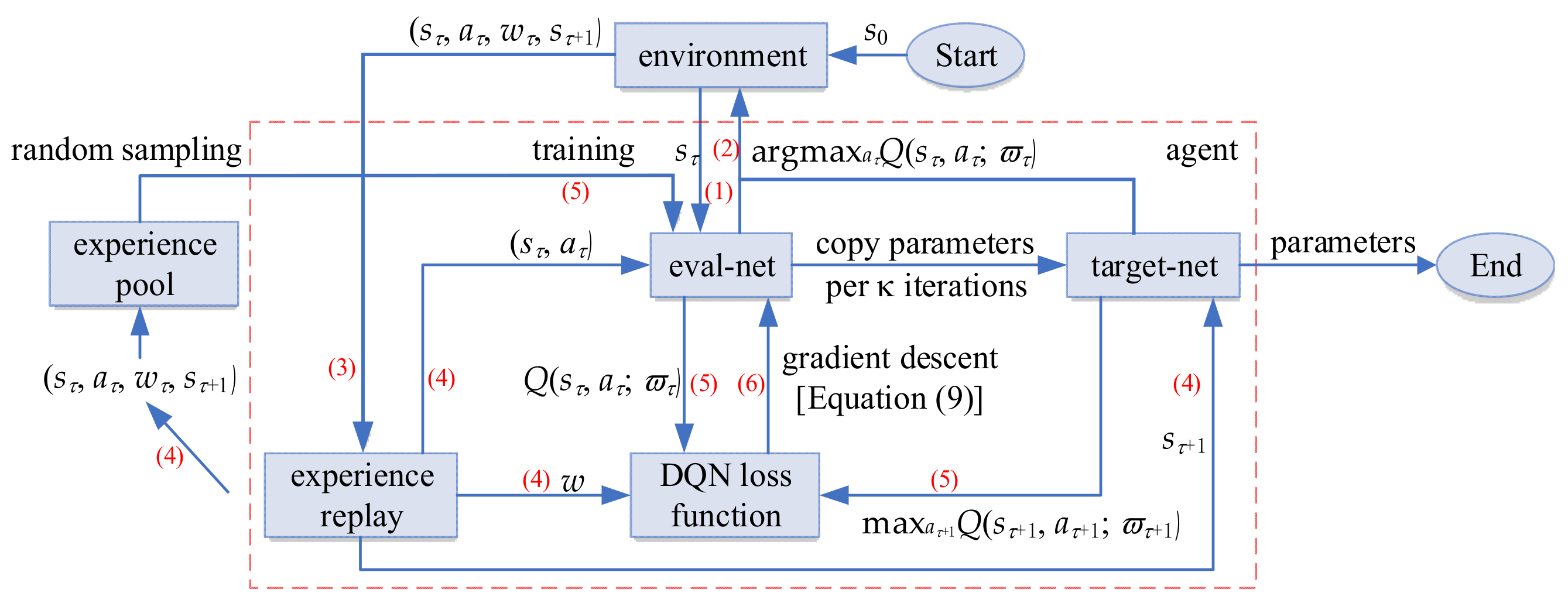
2.2. Deep Q Network Algorithm
3. Transmission Network Expansion Planning Model
3.1. Objective Function
3.2. Constraints
3.3. N-k Fault Power Flow Calculation Model
3.4. EENS Cost Considering the Fault Severity
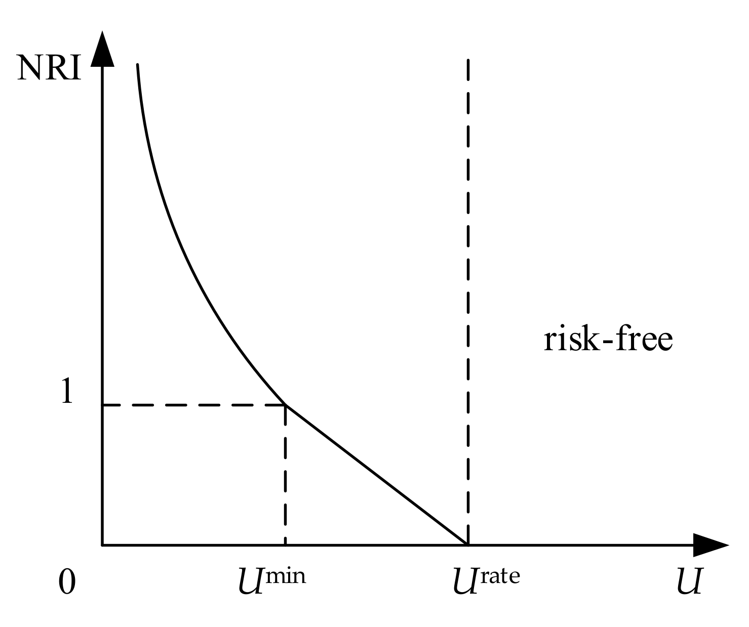
3.5. The Average Normalized Risk Index of Bus Voltages
4. Flexible TNEP Based on DQN Algorithm
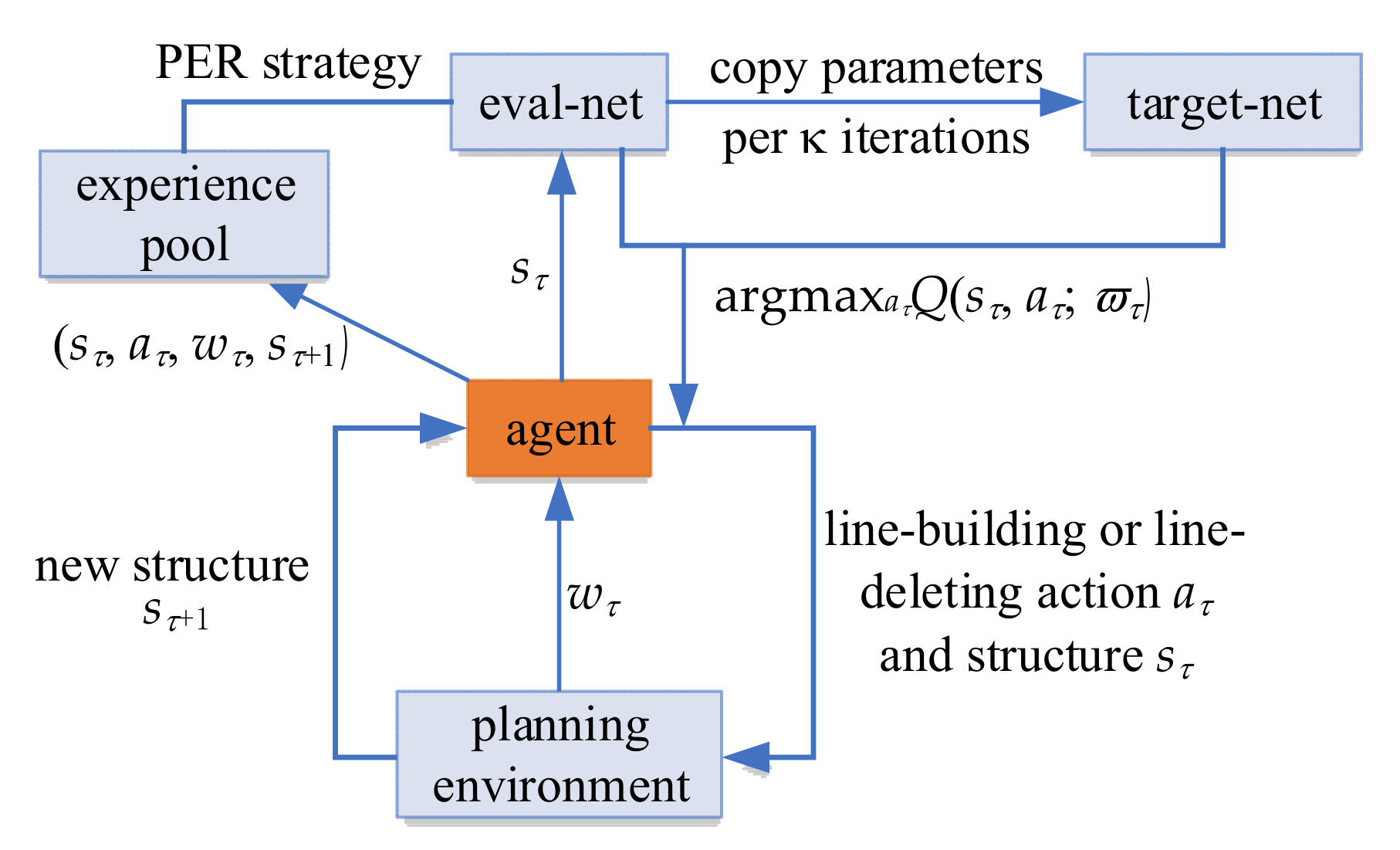
4.1. Algorithm Architecture Design
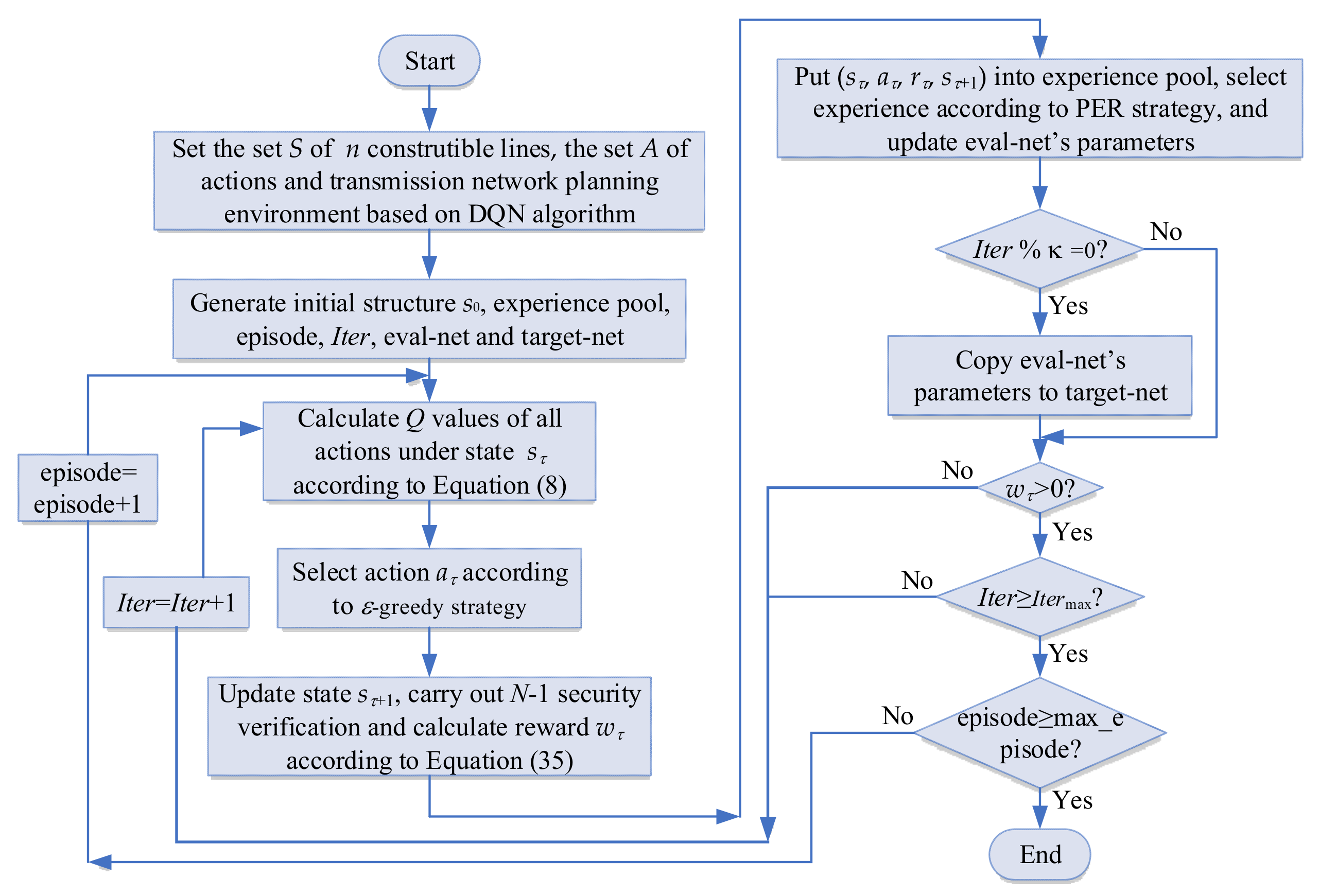
4.2. Planning Process
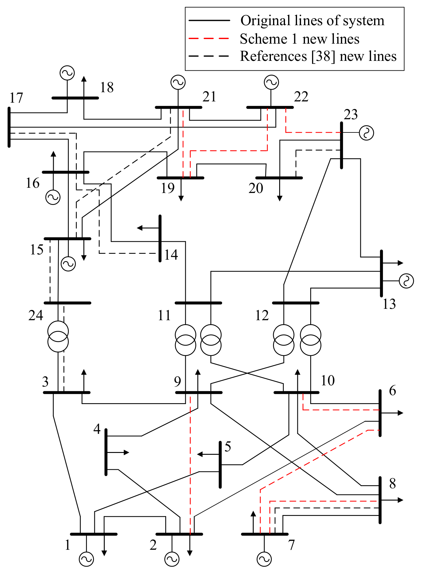
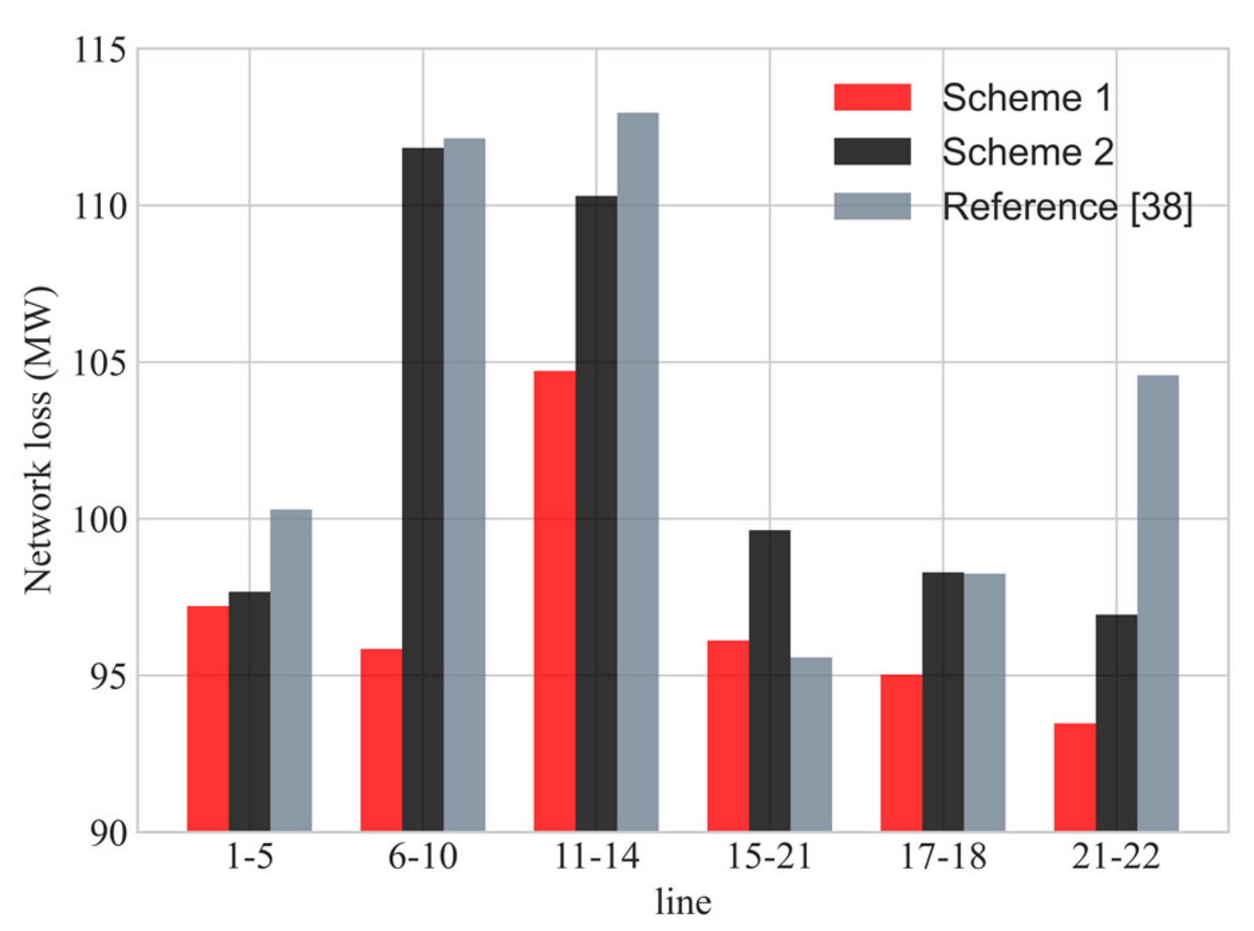
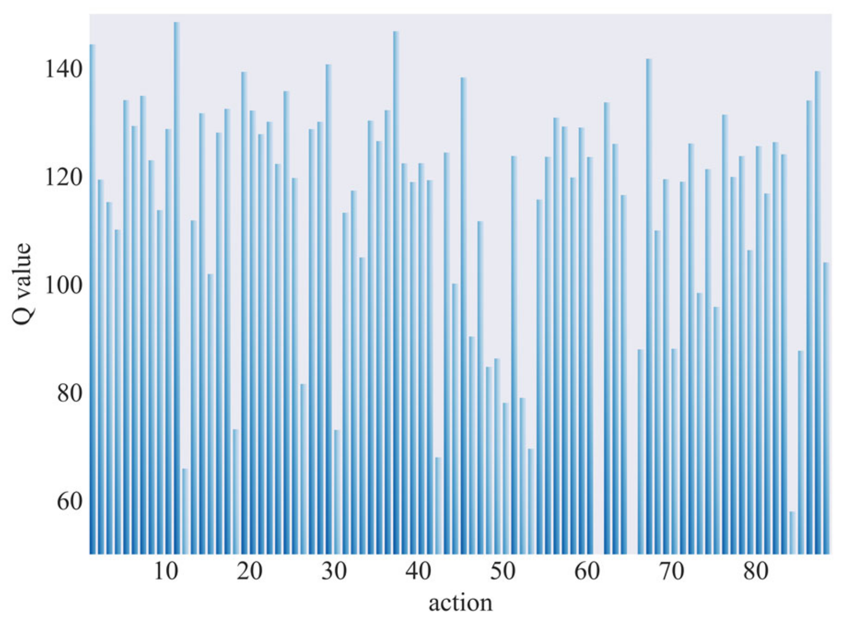
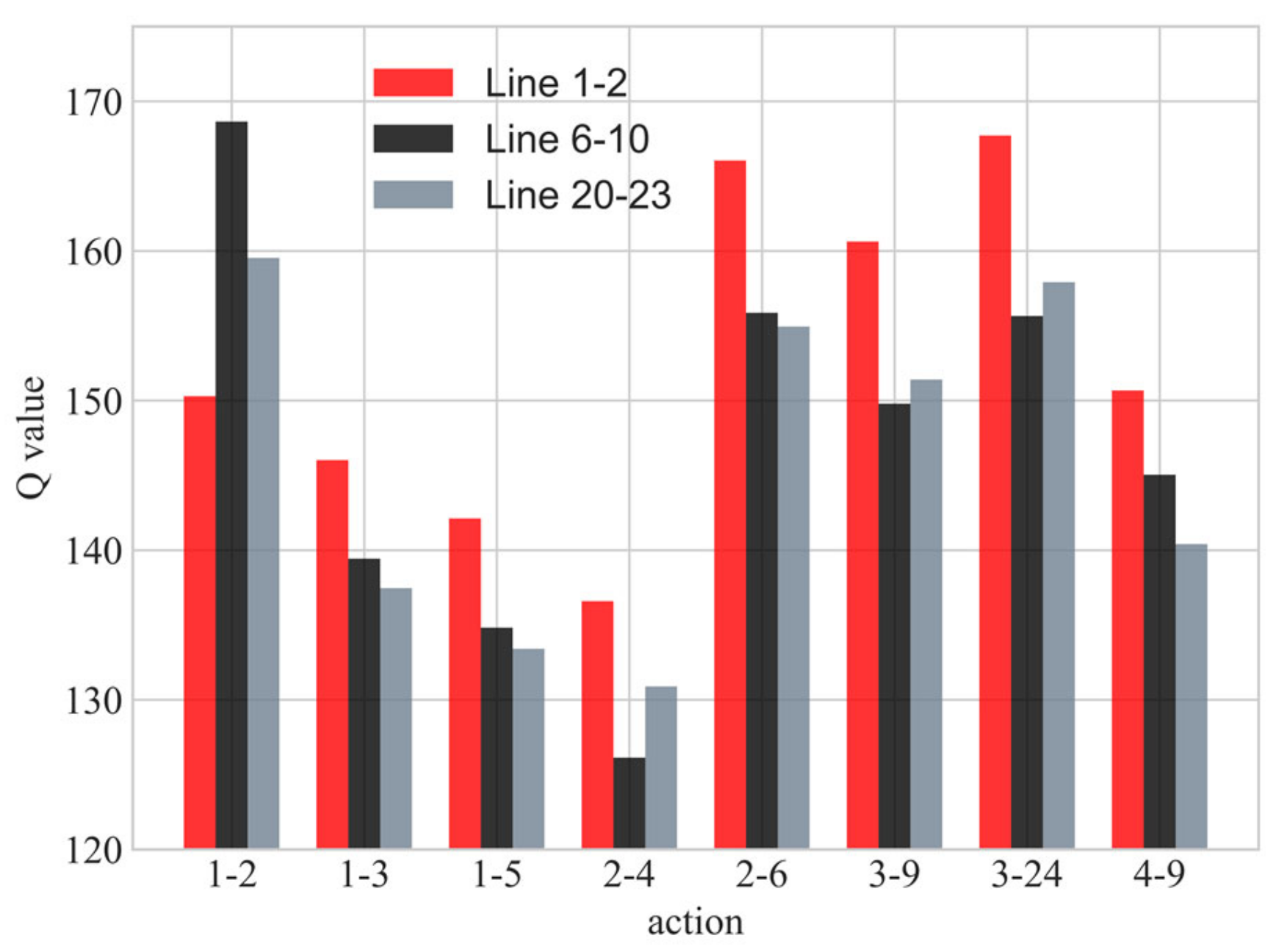
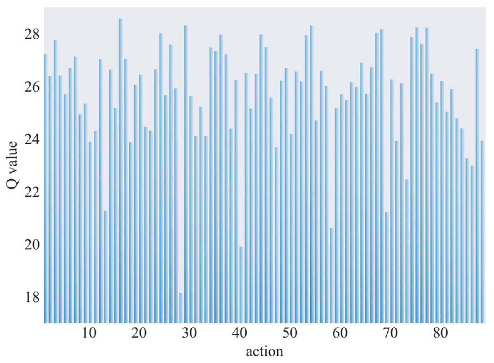
5. Case Study
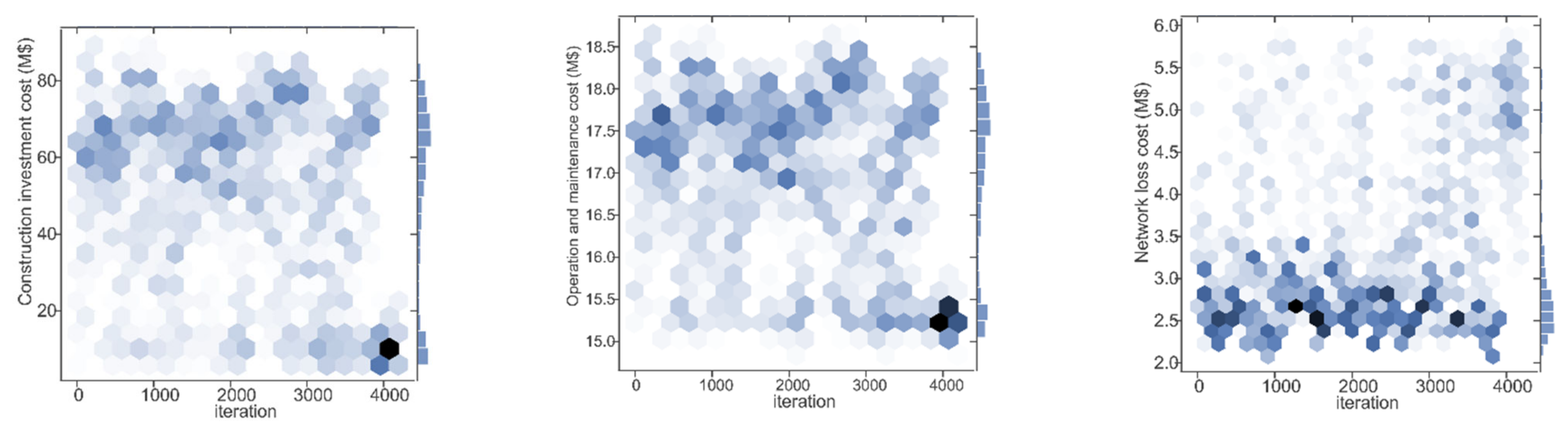
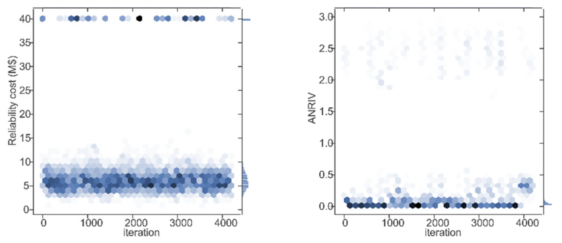
5.1. Experiment 1
5.2. Experiment 2
5.3. Experiment 3
6. Conclusions
Author Contributions
Funding
Acknowledgments
Conflicts of Interest
Nomenclature
| Sets and Indices | |
| π | Set of strategies |
| S | Set of states, for example S = {l1, l2, …, ln} |
| A | Set of actions |
| w | Set of feedbacks |
| W | Set of rewards |
| Q | Set of Q values |
| π* | Set of optimal strategies |
| Ψ | Set of lines that have been built |
| c(i) | Set of all end buses with i as the head bus |
| Φ | Set of transmission network operating states |
| τ | Action index |
| h | The h-th line |
| l | Line index |
| i,j | Bus index |
| e | Equipment index |
| Variables | |
| aτ | Reinforcement learning agent actions |
| sτ | Reinforcement learning states |
| Rτ | Current action reward |
| μ | Random number in the interval [0, 1] |
| d | Current action number |
| Eπ | Mathematical expectation under strategyπ |
| Qπ(s,a) | State–action value function |
| Q*(s,a) | Optimal state–action value function |
| π(s) | ε-greedy action selection strategy |
| Qmax | Optimal action’s Q value |
| Qeval | Q value of eval-net |
| Qtarget | Q value of target-net |
| ϖ | eval-net’s weight |
| L(ϖ) | eval-net’s loss |
| Pτ | Priority of experience τ |
| Δτ | TD error |
| rank(|Δτ|) | Elements of |Δτ| sorted from the maximum to minimum |
| f(sτ) | Comprehensive equivalent cost |
| Cin | Construction investment cost |
| Co | Operation and maintenance cost |
| Closs | Network loss cost |
| CEENS | Reliability cost |
| ζANRIV | Flexibility index ANRIV |
| λin | Annual coefficient of fixed investment cost of the line |
| βl | Binary variable, βl = 1 means line l has been constructed, 0 otherwise |
| PG,i | Total active power output of all generators at bus i |
| H | Total number of lines between bus i and j |
| Iij,h | Current of the h-th line between bus i and j |
| rij,h | Resistance of the h-th line between bus i and j |
| Pload,i | Active power consumed at bus i |
| bij,h | Susceptance of the h-th line between bus i and j |
| θi | Voltage phase angle at bus i |
| , | Lower and upper bound of active power output of all generators at bus i |
| Pij,h | Active power flow of the h-th line between bus i and j |
| Upper bound of active power flow allowable transmission capacity | |
| Ui | Voltage amplitude at bus i |
| , | Lower and upper bound of voltage amplitude at bus i |
| fz | Load shedding under fault state z |
| Pi,z | Load shedding at bus i under fault state z |
| PG,i,z | Sum of the active power output of all generators at bus i under fault state z |
| θ j,z | Voltage phase angle at bus i under fault state z |
| Pij,h,z | Active power flow of the h-th line between bus i and j under fault state z |
| δe | Operation state of equipment e, δe=0 represents equipment e is out of service |
| pf,e | Forced stop rate of equipment e |
| PG,e | Active power output of generator set e under normal operation |
| Mz | Operation state z of the transmission network |
| p(z) | Occurrence probability of state z |
| n(Mz) | Number of samplings of state z |
| PEENS | Annual load shedding |
| Pi,z | Power shortage of bus i under state z |
| ζ V,i | NRI of the voltage at bus i |
| F | Sum of the number of generators and lines |
| Constants | |
| γ | Decay factor of future rewards |
| D | Upper bound of the action number |
| α | Learning rate |
| Γ | Size of the playback experience pool |
| φ | Degree of priority usage |
| cl | Investment cost of unit length construction |
| ξ | expected return on investment |
| y0 | Service life of the investment |
| y1 | Construction life of the planning scheme |
| n | Number of constructible lines |
| Ll | Length of line l |
| λo | Annual coefficient of operation and maintenance cost of the line |
| KG | Unit power generation cost |
| T | Annual maximum load utilization hours |
| N | Number of buses |
| ntotal | Total number of samplings |
| Kloss | Unit network power loss price |
| KEENS | Unit load shedding price |
| ηANRIV | Coefficient that balances the influence of the ζANRIV on the objective function |
Appendix A

| Number | Line | Cost/M$ | Number | Line | Cost/M$ |
|---|---|---|---|---|---|
| 39 | 1–4 | 1.12 | 64 | 7–9 | 2.26 |
| 40 | 1–7 | 2.03 | 65 | 7–10 | 1.72 |
| 41 | 1–8 | 2.36 | 66 | 8–10 | 1.31 |
| 42 | 1–9 | 1.75 | 67 | 11–15 | 1.51 |
| 43 | 2–3 | 2.82 | 68 | 11–23 | 2.40 |
| 44 | 2–5 | 0.83 | 69 | 12–14 | 1.48 |
| 45 | 2–7 | 0.86 | 70 | 12–15 | 2.07 |
| 46 | 2–8 | 1.28 | 71 | 13–14 | 1.76 |
| 47 | 2–9 | 1.84 | 72 | 13–15 | 2.42 |
| 48 | 2–10 | 1.72 | 73 | 13–20 | 1.49 |
| 49 | 3–4 | 1.08 | 74 | 14–15 | 0.67 |
| 50 | 3–5 | 2.10 | 75 | 14–19 | 0.02 |
| 51 | 3–6 | 3.22 | 76 | 14–20 | 0.82 |
| 52 | 3–8 | 3.41 | 77 | 15–19 | 0.93 |
| 53 | 3–10 | 2.38 | 78 | 15–20 | 1.36 |
| 54 | 4–5 | 1.08 | 79 | 16–18 | 0.89 |
| 55 | 4–6 | 2.45 | 80 | 16–19 | 0.89 |
| 56 | 4–10 | 1.72 | 81 | 16–20 | 1.36 |
| 57 | 5–6 | 1.56 | 82 | 17–19 | 1.29 |
| 58 | 5–7 | 1.37 | 83 | 18–19 | 1.11 |
| 59 | 5–8 | 1.42 | 84 | 19–21 | 0.67 |
| 60 | 5–9 | 1.02 | 85 | 19–22 | 0.88 |
| 61 | 6–7 | 1.36 | 86 | 20–21 | 0.80 |
| 62 | 6–8 | 0.75 | 87 | 20–22 | 0.67 |
| 63 | 6–9 | 1.82 | 88 | 22–23 | 0.69 |
References
- Quintero, J.; Zhang, H.; Chakhchoukh, Y.; Vittal, V.; Heydt, G.T. Next generation transmission expansion planning framework: Models, tools, and educational opportunities. IEEE Trans. Power Syst. 2014, 29, 1911–1918. [Google Scholar] [CrossRef]
- Zhang, X.; Conejo, A.J. Candidate line selection for transmission expansion planning considering long- and short-term uncertainty. Int. J. Electr. Power Energy. Syst. 2018, 100, 320–330. [Google Scholar] [CrossRef]
- Nnachi, G.; Richards, C. A com-prehensive state-of-the-art survey on the transmission network expansion planning optimization algorithms. IEEE Access 2019, 7, 123158–123181. [Google Scholar]
- Garver, L.L. Transmission network estimation using linear programming. IEEE Trans. Power App. Syst. 1970, PAS-89, 1688–1697. [Google Scholar] [CrossRef]
- Seifu, A.; Salon, S.; List, G. Optimization of transmission line planning including security constraints. IEEE Trans. Power Syst. 1989, 4, 1507–1513. [Google Scholar] [CrossRef]
- Chen, B.; Wang, L. Robust Transmission planning under uncertain generation investment and retirement. IEEE Trans. Power Syst. 2016, 31, 5144–5152. [Google Scholar] [CrossRef]
- Liang, Z.; Chen, H.; Wang, X.; Ibn Idris, I.; Tan, B.; Zhang, C. An extreme scenario method for robust transmission expansion planning with wind power uncertainty. Energies 2018, 11, 2116. [Google Scholar] [CrossRef]
- Zhao, J.H.; Dong, Z.Y.; Lindsay, P.; Wong, K.P. Flexible transmission expansion planning with uncertainties in an electricity market. IEEE Trans. Power Syst. 2009, 24, 479–488. [Google Scholar] [CrossRef]
- Akbari, T.; Rahimikian, A.; Kazemi, A. A multi-stage stochastic transmission expansion planning method. Energy Convers. Manage. 2011, 52, 2844–2853. [Google Scholar] [CrossRef]
- Alizadeh, B.; Jadid, S. Reliability constrained coordination of generation and transmission expansion planning in power systems using mixed integer programming. IET Gener. Transm. Distrib. 2011, 5, 948–960. [Google Scholar] [CrossRef]
- Feng, Z.K.; Niu, W.J.; Cheng, C.T.; Liao, S.L. Hydropower system operation optimization by discrete differential dynamic programming based on orthogonal experiment design. Energy 2017, 126, 720–732. [Google Scholar] [CrossRef]
- Zakeri, A.; Abyaneh, H. Transmission expansion planning using TLBO algorithm in the presence of demand response resources. Energies 2017, 10, 1376. [Google Scholar] [CrossRef]
- Gallego, L.A.; Garcés, L.P.; Rahmani, M.; Romero, R.A. High-performance hybrid genetic algorithm to solve transmission network expansion planning. IET Gener. Transm. Distrib. 2017, 11, 1111–1118. [Google Scholar] [CrossRef]
- Fuerte Ledezma, L.F.; Gutiérrez Alcaraz, G. Hybrid binary PSO for transmission expansion planning considering N-1 security criterion. IEEE Lat. Am. Trans. 2020, 18, 545–553. [Google Scholar] [CrossRef]
- Cheng, L.; Yu, T. A new generation of AI: A review and perspective on machine learning technologies applied to smart energy and electric power systems. Int. J. Energ. Res. 2019, 43, 1928–1973. [Google Scholar] [CrossRef]
- Wang, J.; Tao, Q. Machine learning: The state of the art. IEEE Intell. Syst. 2008, 23, 49–55. [Google Scholar] [CrossRef]
- Hu, W.; Zheng, L.; Min, Y.; Dong, Y.; Yu, R.; Wang, L. Research on power system transient stability assessment based on deep learning of big data technique. Power Syst. Technol. 2017, 41, 3140–3146. [Google Scholar]
- Cheng, L.; Yu, T. Dissolved gas analysis principle-based intelligent approaches to fault diagnosis and decision making for large oil-immersed power transformers: A survey. Energies 2018, 11, 913. [Google Scholar] [CrossRef]
- Ryu, S.; Noh, J.; Kim, H. Deep neural network based demand side short term load forecasting. Energies 2017, 10, 3. [Google Scholar] [CrossRef]
- Tan, M.; Yuan, S.; Li, S.; Su, Y.; Li, H.; He, F. Ultra-short-term industrial power demand forecasting using LSTM based hybrid ensemble learning. IEEE Trans. Power Syst. 2020, 35, 2937–2948. [Google Scholar] [CrossRef]
- Xiang, L.; Zhao, G.; Li, Q.; Hao, W.; Li, F. TUMK-ELM: A fast unsupervised heterogeneous data learning approach. IEEE Access 2018, 7, 35305–35315. [Google Scholar] [CrossRef]
- Littman, M.L. Reinforcement learning improves behaviour from evaluative feedback. Nature 2015, 521, 445–451. [Google Scholar] [CrossRef]
- Silver, D.; Huang, A.; Maddison, C.; Guez, A.; Sifre, L.; Van Den Driessche, G.; Schritwieser, J.; Antonoglou, L.; Panneershelvam, V.; Lanctot, M.; et al. Mastering the game of Go with deep neural networks and tree search. Nature 2016, 529, 484–489. [Google Scholar] [CrossRef]
- Mnih, V.; Kavukcuoglu, K.; Silver, D.; Rusu, A.A.; Veness, J.; Bellermare, M.G.; Graves, A.; Riedmiller, M.; Fidjeland, A.K.; Ostrovski, G.; et al. Human-level control through deep reinforcement learning. Nature 2015, 518, 529–533. [Google Scholar] [CrossRef]
- Ji, Y.; Wang, J.; Xu, J.; Fang, X.; Zhang, H. Real-time energy management of a microgrid using deep reinforcement learning. Energies 2019, 12, 2291. [Google Scholar] [CrossRef]
- Yu, T.; Wang, H.Z.; Zhou, B.; Chan, K.W.; Tang, J. Multi-agent correlated equilibrium Q(λ) learning for coordinated smart generation control of interconnected power grids. IEEE Trans. Power Syst. 2015, 30, 1669–1679. [Google Scholar] [CrossRef]
- Xi, L.; Yu, L.; Xu, Y.; Wang, S.; Chen, X. A novel multi-agent DDQN-AD method-based distributed strategy for automatic generation control of integrated energy systems. IEEE Trans. Sustain. Energy 2020, 11, 2417–2426. [Google Scholar] [CrossRef]
- Cao, J.; Zhang, W.; Xiao, Z.; Hua, H. Reactive power optimization for transient voltage stability in energy internet via deep reinforcement learning approach. Energies 2019, 12, 1556. [Google Scholar] [CrossRef]
- Hong, S.; Cheng, H.; Zeng, P. An N-k analytic method of composite generation and transmission with interval load. Energies 2017, 10, 168. [Google Scholar] [CrossRef]
- Zhang, Y.; Wang, J.; Li, Y.; Wang, X. An extension of reduced disjunctive model for multi-stage security-constrained transmission expansion planning. IEEE Trans. Power Syst. 2018, 33, 1092–1094. [Google Scholar] [CrossRef]
- Kim, W.-W.; Park, J.-K.; Yoon, Y.-T.; Kim, M.-K. Transmission expansion planning under uncertainty for investment options with various lead-times. Energies 2018, 11, 2429. [Google Scholar] [CrossRef]
- Arabali, A.; Ghofrani, M.; Etezadi-Amoli, M.; Fadali, M.S.; Moeini-Aghtaie, M. A multi-objective transmission expansion planning framework in deregulated power systems with wind generation. IEEE Trans. Power Syst. 2014, 29, 3003–3011. [Google Scholar] [CrossRef]
- Kamyab, G.-R.; Fotuhi-Firuzabad, M.; Rashidinejad, M. A PSO based approach for multi-stage transmission expansion planning in electricity markets. Int. J. Electr. Power Energy Syst. 2014, 54, 91–100. [Google Scholar] [CrossRef]
- Qiu, J.; Zhao, J.; Wang, D. Flexible multi-objective transmission expansion planning with adjustable risk aversion. Energies 2017, 10, 1036. [Google Scholar] [CrossRef]
- Schaul, T.; Quan, J.; Antonoglou, I.; Silver, D. Prioritized experience replay. In Proceedings of the International Conference on Learning Representations 2016, San Juan, Puerto Rico, 2–4 May 2016. [Google Scholar]
- Ni, M.; McCalley, J.D.; Vittal, V.; Tayyib, T. Online risk-based security assessment. IEEE Trans. Power Syst. 2003, 18, 258–265. [Google Scholar] [CrossRef]
- Subcommittee, P.M. IEEE Reliability Test System. IEEE Trans. Power App. Syst. 1979, PAS-98, 2047–2054. [Google Scholar] [CrossRef]
- Zhang, H.; Vittal, V.; Heydt, G.T.; Quintero, J. A mixed-integer linear programming approach for multi-stage security-constrained transmission expansion planning. IEEE Trans. Power Syst. 2012, 27, 1125–1133. [Google Scholar] [CrossRef]


| Planning Scheme | Cin/M$ | Co/M$ | Closs/M$ | CEENS/M$ | ζANRIV | f(sτ)/M$ | |
|---|---|---|---|---|---|---|---|
| Scheme 1 | 6–7,19–21,19–22,7–8, 2–9,22–23,6–10 | 6.73 | 15.02 | 4.66 | 4.27 | 0.21 | 37.22 |
| Scheme 2 | 6–7,19–21,19–22,18–21, 3–6,1–5,20–23 | 8.99 | 15.17 | 4.83 | 1.95 | 0.40 | 43.35 |
| Reference [38] | 3–24,7–8,14–16,15–21, 15–24,16–17,20–23 | 10.44 | 15.20 | 4.62 | 4.14 | 0.72 | 59.18 |
| Constructed Line | Q Value | Cin/M$ | CEENS/M$ | ζANRIV | f(sτ)/M$ |
|---|---|---|---|---|---|
| 7–8 | 148.48 | 3.55 | 5.51 | 0.39 | 39.86 |
| 11–14 | 139.27 | 4.65 | 4.63 | 0.45 | 42.16 |
| 17–18 | 73.00 | 3.51 | 7.72 | 0.49 | 46.25 |
| Expansion Scheme | Cin/M$ | CEENS/M$ | ζANRIV | f(sτ)/M$ |
|---|---|---|---|---|
| 6–7,19–21,19–22,11–14, 19–20,6–10,3–24 | 8.94 | 2.85 | 0.24 | 39.20 |
| 6–7,19–21,19–22,11–14, 19–20,6–10,2–8 | 8.22 | 2.60 | 0.25 | 38.22 |
| 6–7,19–21,19–22,11–14, 19–20,6–10,19–20 | 8.70 | 5.38 | 0.29 | 43.72 |
| Scheme 1 | 6.73 | 4.27 | 0.21 | 37.22 |
| Constructed Line | Q Value | Cin/M$ | CEENS/M$ | ζANRIV | f(sτ)/M$ |
|---|---|---|---|---|---|
| 10–11 | 28.57 | 8.73 | 4.90 | 0.19 | 39.71 |
| 9–11 | 26.64 | 8.73 | 5.67 | 0.18 | 40.25 |
| 13–23 | 24.31 | 10.33 | 5.57 | 0.21 | 41.95 |
Publisher’s Note: MDPI stays neutral with regard to jurisdictional claims in published maps and institutional affiliations. |
© 2021 by the authors. Licensee MDPI, Basel, Switzerland. This article is an open access article distributed under the terms and conditions of the Creative Commons Attribution (CC BY) license (http://creativecommons.org/licenses/by/4.0/).
Share and Cite
Wang, Y.; Chen, L.; Zhou, H.; Zhou, X.; Zheng, Z.; Zeng, Q.; Jiang, L.; Lu, L. Flexible Transmission Network Expansion Planning Based on DQN Algorithm. Energies 2021, 14, 1944. https://doi.org/10.3390/en14071944
Wang Y, Chen L, Zhou H, Zhou X, Zheng Z, Zeng Q, Jiang L, Lu L. Flexible Transmission Network Expansion Planning Based on DQN Algorithm. Energies. 2021; 14(7):1944. https://doi.org/10.3390/en14071944
Chicago/Turabian StyleWang, Yuhong, Lei Chen, Hong Zhou, Xu Zhou, Zongsheng Zheng, Qi Zeng, Li Jiang, and Liang Lu. 2021. "Flexible Transmission Network Expansion Planning Based on DQN Algorithm" Energies 14, no. 7: 1944. https://doi.org/10.3390/en14071944
APA StyleWang, Y., Chen, L., Zhou, H., Zhou, X., Zheng, Z., Zeng, Q., Jiang, L., & Lu, L. (2021). Flexible Transmission Network Expansion Planning Based on DQN Algorithm. Energies, 14(7), 1944. https://doi.org/10.3390/en14071944