Article

Evaluating Variability of Ground Thermal Conductivity within a Steep Site by History Matching Underground Distributed Temperatures from Thermal Response Tests

1
Department of Environmental Engineering, Faculty of Engineering, Hokkaido University, N13-W8, Sapporo 060-8628, Japan
2
Mechanical Power Engineering Department, Faculty of Engineering at Shoubra, Benha University, Shoubra 11629, Egypt
3
Inoac Housing & Construction Materials, Daiho-4tyome, Nagoya 456-0062, Japan
*
Author to whom correspondence should be addressed.
Energies 2021, 14(7), 1872; https://doi.org/10.3390/en14071872
Submission received: 10 February 2021 / Revised: 22 March 2021 / Accepted: 24 March 2021 / Published: 28 March 2021
(This article belongs to the Special Issue Thermal Response Tests for Shallow Geothermal Systems)

Abstract

:
The variability of ground thermal conductivity, based on underground conditions, is often ignored during the design of ground-source heat pump systems. This study shows a field evidence of such site-scale variations through thermal response tests in eight borehole heat exchangers aligned at a site on a terrace along the foothills of mountains in northern Japan. Conventional analysis of the overall ground thermal conductivity along the total installation length finds that the value at one borehole heat exchanger is 2.5 times that at the other seven boreholes. History matching analysis of underground distributed temperature measurements generates vertical partial ground thermal conductivity data for four depth layers. Based on the moving line heat source theory, the partial values are generally within a narrow range expected for gravel deposits. Darcy velocities of groundwater are estimated to be 74–204 m/y at the borehole with high conductivity, increasing in the shallow layers above a depth of 41 m. In contrast, the velocities at the other seven boreholes are one-to-two orders of magnitude smaller with no trend. These high and low velocity values are considered for the topography and permeability. However, the relatively slow groundwater velocities might not apparently increase the partial conductivity.

1. Introduction

The ground thermal conductivity is a key determinant of the required size of a borehole heat exchanger (BHE) when designing and planning ground-source heat pump (GSHP) systems. This geothermal property is defined as a thickness-weighted average of the effective thermal conductivity of the soils/rocks comprising the formation at a site. The effective thermal conductivity of individual components ranges between <1 W/(m⋅K) for unsaturated fine sediments and >4 W/(M·K) for crystallized rocks, depending on the particles, porosity, and water content [1,2]. The design guideline of ASHRAE (American Society of Heating, Refrigerating and Air-Conditioning Engineers) specifies that a required length of a BHE in limestone with thermal conductivity of 3.1 W/(m·K) should be approximately half of that in unconsolidated clay of 1.2 W/(m·K) for the same conditions of thermal pulses in six hours [3]. The differences in BHE lengths became longer as the spans for thermal pulses became larger. Although GSHPs are established renewable-energy-based systems contributing to energy-saving and CO2 emission reduction [4], the problem is that the capital costs of installing BHEs often exceed those of competing systems conventional air-source heat pumps [5]. Therefore, it is critical to obtain realistic estimates of the ground thermal conductivity at a site to determine the required lengths of BHEs, especially in the initial stage of designing and planning a heating, ventilation, and air-conditioning system [6].
Thermal response testing (TRT) is a standard method for evaluating ground thermal conductivity in-situ. It was originally developed in Sweden [7], and has since been standardized in various countries, such as the USA [8], Germany [9], and Japan [10], and by the international association [11]. The measurement and analysis methodologies are simple for practice. The test is conducted by circulating fluids in BHEs at a constant heating rate, and the temperature of the circulating fluids is observed at the shanks of inlet and outlet U-tubes. The temperature changes were analyzed based on heat-transfer theory assuming that the testing BHE is an infinite line source (ILS) in the ground [12]. This conventional TRT can provide ground thermal conductivity straightforwardly without significant computational effort.
In several decades, the methodology has been developed to improve its accuracy by incorporating other theoretical solutions for infinite cylindrical sources [1,11,13], and finite line sources [11,14]. The methodology used for determining ground thermal conductivity is an uncertain variable that could be modified to obtain sufficient agreements between measurements and calculations. The sum of squared error or the root mean squared error in the calculations is usually used for evaluating the agreements [15]. If a temporal series of fluid and/or soil temperatures are compared between calculations and measurements, the inversion method is called history matching analysis [13]. The literature review found that the share of applications of cylindrical and line source theory were 25% and 75%, respectively [16]. Complicated test conditions have also been accommodated by adopting numerical simulation [17,18,19]. The numerical modeling is available to not only estimate ground thermal conductivity, but also other parameters, such as thermal capacity [20], and borehole thermal resistance [21]. The numerical models are also used to estimate spatial distributions of ground thermal conductivity in a region [22]. Another testing approach based on variable heating power was also proposed in the same concept of water well pumping tests [23].
Ground thermal conductivity is potentially variable depending on the geological and groundwater conditions. A known issue in shallow geothermal utilization is uncertainty about such underground variation within site. TRT provides only one value at a location for the installation length of a test BHE, and only one test is usually conducted for cost reasons. Given the limited information, site-scale variability is assumed to be negligible in the practical design and planning of GSHP systems. This assumption might be valid under the following three conditions: The installation length of the BHE is fixed to neglect vertical changes; the formation is stratified, and each layer of a particular geologic component is continuous for negligible changes in horizonal directions; moreover, groundwater flows are slow enough to neglect advective heat transfer in the soil and rock.
The appropriate length of a BHE can be found for a site-dependent condition of vertical change in ground thermal conductivity through analysis of underground data collected by distributed temperature sensors (DTSs). DTSs are installed in a BHE to measure continuous depth-resolved temperature measurements during the heating phase, as called distributed TRT (DTRT). DTRT is classified in terms of installation number and location of DTSs; (1) a single DTS outside U-tubes [24], (2) a looped DTS attached along U-tubes [25], (3) a DTS into an inlet or outlet U-tube [13], and (4) a pair of DTS into inlet and outlet U-tubes [26,27]. Instead of circulating fluids at constant heating, the electric current-carrying copper wire is also used as a heat source along the DTSs [28,29,30]. The studies above have demonstrated to estimate vertical profiles of ground thermal conductivity from the distributed temperature data. A part of the studies also analyzed the profiles of borehole thermal resistance [26]. The heating cable TRTs were available in the boreholes at geotechnical investigations to cut the drilling costs [31].
This study focuses on the advection in TRTs by groundwater flows, the third listed effect on ground thermal conductivity. Previous field and laboratory studies of TRTs have shown advection to increase the ground thermal conductivity [32]. As an example, the apparent value was 9.14 W/(m·K) at a site of high groundwater flows in Japan [33]. The site was located in a basin surrounding the mountains with large precipitations, and natural groundwater flows at a site were estimated at 2750 m/y in the shallow layer [34]. Artificial flows of groundwater occur around water wells, potentially increasing the ground thermal conductivity. The authors demonstrated the DTRT near the pumping well, indicating the value increased from 2.00 W/(m.K) to 3.19 W/(m·K) [35]. In the guideline [36], the specific heat extraction per meter in depth is 80–100 W/m for “strong groundwater flow in gravel and sand,” and the value is almost double the value for no flow, 55–65 W/m. This means that the required length of a BHE is potentially designed to be 200% shorter, if groundwater flows actively. A theoretical study [37] indicated that the advection effect is not negligible when the Darcy velocity (specific discharge) is over 10−8 m/s (2 m/y), which is often the case in sedimentary basins. However, an actual effect of groundwater flows on the life cycle costs of a household GSHP system in Japan would appear when the Darcy velocity of groundwater is the order of 101 m/y or more [38]. The advection effects were also validated for multiple BHEs in numerical studies [39,40].
Although several research papers regarding TRTs was available, few studies have examined the variability of ground thermal conductivity on the intra-site scale for the construction of multiple BHEs, i.e., with an interval of several meters in a range of 101 to 102 m. One reason for the lack of relevant field data is the additional cost of conducting multiple TRTs at each site, as described above. Furthermore, the site topography might limit studies, with building sites often being located on flat land with slopes too gentle for significant advection. For example, the previous study demonstrated TRTs at six BHEs of different configurations in terms of U-tube and borehole diameter, indicating the small variability of ground thermal conductivity between 1.2–1.6 W/(m·K) [41]. However, in the steep reliefs, as often seen in Japan and other mountainous and hilly countries, high hydraulic gradients make rapid groundwater flows common, as described above. In such a site of high groundwater flows, it is expected to design reasonable lengths of BHEs, compared with no groundwater flows [33,34]. On the other hand, we also assumed that the groundwater flows might be uniform in space depending on the porosity distribution in the aquifer, because the sediments become coarser and more permeable around the foothills of mountains [42]. In such uniformity of groundwater flows, ground thermal conductivity is apparently changed. Consequently, the advection might affect more significantly the performances of multiple BHEs than in the flat plains.
This study aimed to evaluate site-scale variability of the ground thermal conductivity through TRTs at eight BHEs aligned at a site in Bibai City, Japan. The site was located on the terraced foothills of nearby mountains. The original purpose of the DTRTs was to compare borehole thermal resistances with respect to thermal performances of different configurations of U-tube, as previously reported [43]. The previous study summarized the ground thermal conductivities of the eight BHEs, indicating that the value at one site was about 2.5 times larger than those at the other seven BHEs. This study demonstrated a method to estimate the vertical changes of partial ground thermal conductivity in each of four layers comprising the formation through history matching analysis of underground distributed temperature data from optic-fiber DTSs. The present study compared the theoretical solutions for an ILS and a moving line source (MLS) [44]. The latter solution provided the partial ground thermal conductivity and Darcy velocity in each layer of the eight BHEs. The statistics represent field evidence for the site-scale variability in properties around steep reliefs.

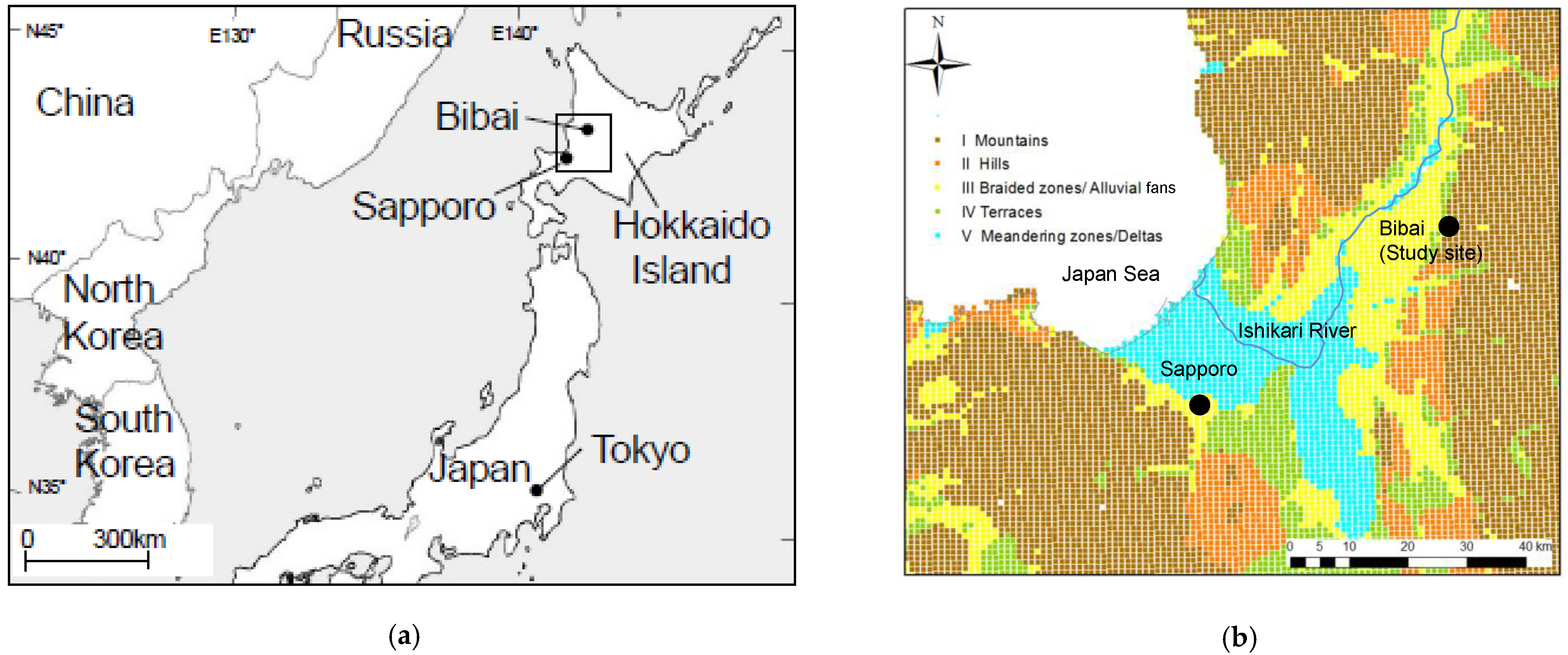
2. Site Descriptions and Test Conditions

The study site was located at 43.32° N, 141.85° E, in Bibai City on Hokkaido, the northernmost island of Japan, as shown in Figure 1a. Figure 1b shows the Ishikari River, one of the island’s longest rivers, flowing from NNE to SSW from the northern mountains. The river’s valley has braided zones and alluvial fans consisting of coarse sediments in the Quaternary and Tertiary periods [45]. Near Sapporo, the island’s capital (population, about 2 million), the river’s flow changes to NE, before reaching the Japan Sea. There are meandering zones of Holocene fine sediments in the fluvial areas around Sapporo.
The study site is located on a small terrace along the foothills of the mountains. Drilling report of the BHEs construction showed that the formation was composed of monotonic gravel deposits, which were transferred mainly from the upper mountains, with some coming from the Ishikari River. Although in-situ measurements of permeability around the site were not obtained, the coarse deposits were assumed to be highly permeable. Also, the sediments were assumed not to be sorted well in the steep topography. This means the porosity related to soil particle distributions might be strongly uniform in the gravel deposits.
Eight BHEs, Nos 1 to 8, were constructed at the site in September 2018 at regular intervals of 4.0 m (except for the 6.5 m distance between Nos 6 and 7), as shown in Figure 2a. Each commonly had an installation depth of 82 m. The U-tubes were made of high-density polyethylene (HDPE), and were buried with silica sand, a typical grout material in Japan. The sand’s thermal properties were assumed to be close to those of the underground gravel deposits. The borehole diameter was 0.126 m for the single U-tubes of Nos. 3 to 8, and 0.139 m for double U-tubes. The eight BHEs were originally constructed to compare different cross-sectional configurations of U-tubes: Conventional circular shape or oval shape, single or double, and with or without a spacer to prevent thermal interference between the inlet and outlet U-tubes. The spacer length Ls was changed to evaluate its effect on thermal performance. Figure 2b shows the schematic cross-section of each BHE: No. 1, circle/double (Cd); No. 2, Cd with a spacer (82 m long) (Cd+); No. 3, circle/single (C); No. 4, C with a spacer (C+); No. 5, oval/single (O); No. 6, O with a spacer (Ls = 10 m, O+); No. 7, O+ (40 m); No. 8, O+ (82 m). The oval U-tube (O) was developed to improve efficiency by increasing the tube outer surface areas in boreholes with the same diameter as Cs boreholes [46].
Optic-fiber DTSs were attached to the surface of inlet and outlet U-tubes installed in each borehole. Each sensor was made of GI62.5 optic fiber (diameter, 125 μm) covered by a spiral metal tube for protection against soil pressure and by flexible plastic for water resistance, as shown in the upper right of Figure 2b. As the sensors were each attached twice, the sensor length in each BHE was 164 m (82 × 2). Each of the two attachments was cross-sectionally opposite. After construction of all the BHEs, the fibers were connected as a sequence from No. 1 to 8, resulting in a total length of over 1300 m. The temperatures on the outer surface of each U-tube were measured at regular 0.5 m depth intervals by the DTSs. The temperatures on the surface were assumed to be those at two opposite points at the same distance from the center, ro. The DTS measurements were performed by using the signal receivers (N4385A type of A.P. Sensing, Co., Ltd., Boeblingen, Germany). The equipment has the advantage of changing the direction to send the optical signals in the DTS regularly to eliminate the fluctuation errors. The errors were also reduced through the filtering based on the Fast Fourier Transform (FFT) procedure, resulting in an averaged accuracy of 0.25 K, as shown in the previous study [47]. This study’s history matching analysis used the average of two temperatures by the DTSs, recorded on the opposing points at each depth T0.
This study conducted conventional TRTs at each of the eight BHEs, as shown in Figure 3. Tap water was injected to fill the U-tubes at a pressure of about 0.1 MPa. The TRT equipment consisted of an electric heater, a circulation pump, a magnetic flow meter, and data acquisition devices. The water was circulated constantly at a flow rate of about 20 L/min. This study used two sets of equipment to save time. The circulating water was also heated at a constant rate of about 4.0 kW in one set of TRT equipment or 4.4 kW in the other. The heating period was 48 h (2 days), except at BHE No. 3 for high ground thermal conductivity, whose period was set at 96 h (4 days) to obtain stable temperature changes, likely due to groundwater flows. The temperatures of the circulating fluids were observed every minute at the shanks of the inlet and outlet U-tubes by Pt100 temperature sensors with an accuracy of 0.1 K.
The testing time schedule was as follows: 2018-10-10 16:01 to 2018-10-12 16:01 in Nos 1 and 3, 2018-10-23 12:31 to 2018-10-25 12:31 in Nos 2 and 6, 2018-10-16 15:31 to 2018-10-18 15:34 in Nos 4 and 8, 2018-10-31 12:53 to 2018-11-2 12:34 in No. 5, and 2018-11-6 15:02 to 2018-11-8 15:19 in No. 7. After heating, observation by the DTSs was maintained to measure recovery to the initial temperature.

3. Methodology for Analysis

First, this study performed conventional TRT analysis to determine overall values of ground thermal conductivity for the total lengths (82 m), λ ¯ in the eight BHEs. The analysis assumed each BHE to be an ILS with a constant heat exchange rate q [W/m], which was calculated from the total input power Q [kW] divided by the installation length L [m]. The total input power Q was calculated from the fluid temperature difference between the inlet and outlet shanks:
Q = ρ w C w v ( T f i n T f o u t ) ,
where ρ w C w is the volumetric heat capacity of the circulating water [J/(m3⋅K)]. v is the circulating flow discharge [m3/s]. The input power Q was confirmed to be kept within a 5% range, due to the fluctuations of T f i n T f o u t , and v , and thus, the average Q was used to calculate q for analysis. We also assumed that the surrounding soil was homogeneous and isotropic. Thus, the change in underground soil temperature Δ T s [K] by heating was calculated as [1]
Δ T s = T s T 0 = q 4 π λ r 2 4 a t e u u d u ,
where T s is the borehole surface temperature [°C], T 0 is the initial soil temperature [°C], λ is the ground thermal conductivity [W/(m⋅K)], a is the thermal diffusivity [m2/s] equal to λ divided by volumetric thermal capacity—which is assumed to be 3 MJ/(K·m3)—   r is radius [m], and t is elapsed testing time [h]. After the time greater than the minimum time, e.g., t > 20 a / r 2 [1], Equation (2) could be approximated for simple calculation as
Δ T s q 4 π λ [ log ( 4 a t r 2 ) γ ] ,
where γ is the Euler constant. Equation (3) indicates that the temperature increased log-linearly with time. Thus, the linear slope κ was determined from least-squares fitting of semi-log plots of the average inlet and outlet temperatures from the PT100 sensors, i.e., T f ¯ = ( T f i n + T f o u t ) / 2 . Considering the coefficient q / 4 π λ in Equation (2) was equal to the slope κ of the measured logarithmic temperatures, λ ¯ was determined as
λ ¯ = q 4 π κ ,
each BHE was not actually an ILS, and the temperature change of the circulating fluid T f ¯ was affected not only by λ ¯ , but also by the borehole thermal resistance Rb [m·K/W]. The value of R b was calculated for the temperature difference between the fluid and borehole surface as
R b = T T 0 q 1 4 π λ ¯ [ ln 4 a × 3600 r b 2 γ ] ,
where T is the intercept of the fitted straight line [°C], for determination of κ above, and represents the temperature at t = 1 h ( log t = 0). The blank value for 3600 was used for an elapsed time of 1 h (3600 s).
Estimation by history matching analysis was next applied using the distributed temperature measurements on the outer surfaces of the U-tubes during heating and recovery. The analysis obtained the vertically partial ground thermal conductivity λ I ,   λ II ,   λ III ,   and   λ IV for layers I (depth; Z = 0–20.5 m), II (20.5–41 m), III (41–61.5 m), and IV (61.5–82 m), respectively. Each layer was assumed to be of equal thickness owing to limited information about the geologic structure, as the monotonic gravelly formation. The heat exchange rate q was also estimated to be constant within, but different among the layers. Vertically partial estimates in each layer were determined to obtain the best agreements for the temperature at the radius r 0 between measurements by DTS and calculations during heating and recovery. Theoretical calculations for soil temperature during recovery were conducted for constant and uniform heating [11]:
Δ T s ( t > t ) = Δ T s ( t ) Δ T s ( t t ) ,
where t is the time at which heating stopped. The recovery period for analysis was defined as the time for the temperature change to drop to 10% or less its peak rate. R M S E was used as a criterion for evaluating agreement between the calculated and measured temperatures [15]:
R M S E = 1 N t ( Δ T o b s Δ T c a l ) 2 ,
where Δ T o b s and Δ T c a l are the observed and calculated temperature changes from the initial temperature, respectively, N is the number (minute counts) of time steps for the history matching. Δ T o b s was obtained by averaging 42 × 2 DTS data at 0.5 m intervals in each 20.5 m thickness.
This study compared partial conductivities between ILS and MLS considering the uncertain effects of groundwater flow. First, the ILS theory in Equation (2) was used, resulting in partial estimates, including groundwater flow effects, i.e., the apparent thermal conductivity. To assess the effect of advection by groundwater flow, this study also applied another solution of the MLS theory instead of Equation (2) [44]:
Δ T s = q 4 π λ 0 π e x p ( U r 2 a cos φ ) 0 4 a t r 2 1 η e x p ( 1 η U 2 r 2 η 16 a 2 ) d η d φ ,
U = ρ w C w ρ C p u
where U is the modified velocity of groundwater [m/s], ρ w C w is the heat capacity of groundwater (4.2 MJ/(m3·K)) and ρ C p is that of the soil (3 MJ/(m3·K)), u is the Darcy velocity (specific discharge) [m/s], and φ is flow direction (angle) [rad]. Integrating Equation (8) with respect to the flow angle φ results in the average temperature change at radius ro. This study assumed a negligible effect of hydraulic dispersion under a rapid groundwater flow to simplify the calculation convergence, as applied in other studies [48]. Soil temperatures were calculated based on Equations (8) and (9), and then the vertical partial properties of λ , q , and log u   were determined using the least R M S E in each layer I, II, III, or IV at the eight BHEs. The Darcy velocity was converted to logarithmic form through parameter optimization, considering that the velocity was potentially variable by several orders of magnitude. The non-linear optimization algorithm “fmincon” in MATLAB was used to obtain the least R M S E , within the following range for each parameter: 1 λ 4 , 10 q 100   ,   0.1 log u 3 . Comparison of the parameters determined using ILS or MLS in each of the four layers aligning with the eight BHEs gives the site-scale variability with respect to the site’s geothermal and hydrogeologic properties.

4. Results

4.1. Conventional TRT Analysis

Table 1 summarizes the test configurations and analysis results, λ ¯ and R b , from conventional TRTs in the eight BHEs, and is modified from Table 1 in our previous paper [43] by the addition of the results for λ ¯ . Conventional estimation of λ ¯ for the same length (82 m) ranged between 1.83 and 2.17, except for BHE No. 3; the average of the other seven BHEs was 1.94 W/(m·K). Considering a 10% error as ordinarily acceptable in conventional TRTs [17,49], the ground thermal conductivity in the seven BHEs was approximately equal to the average value, which itself was equal to reference values for dense gravel deposits [1,2,8]. However, at BHE No. 3, the estimate of λ ¯ was 4.93 W/(m·K), which was about 2.5 times greater than that at the other BHEs.
Figure 4 shows the changes of T f ¯ measured by the PT100 sensors in the eight BHEs. T f ¯ increased linearly in logarithmic time except at BHE No. 3. The intercepts of the fitted lines for T f ¯ at the other seven BHEs depended on the heating rate in the two equipment sets, and the borehole thermal resistance related to the U-tube configuration. The plots for the seven BHEs showed slopes that were not clearly different from each other, indicating small variability of λ ¯ . In contrast, T f ¯ at BHE No. 3 also increased with time, but not linearly as at the other BHEs; it almost converged as the heating time progressed. The small increase in T f ¯ was probably due to the effects of groundwater flow, as discussed later.
In-situ Rb values were compared and discussed in detail in the previous study [43]. This paper briefly summarizes the comparison. In Table 1, the in-situ Rb value of the oval/single(O) U-tube (No. 5) was about 10% lower than that of the circle/single(C) U-tube (No. 3), indicating the oval U-tube more effectively enhanced the thermal performance of the BHEs than the circular U-tube. However, the in-situ Rb value of oval/single tube (No. 5) was not lower than that of the more expensive circle/double (Cd) (No. 1), and thus, an oval-U tube is expected to be cost-effective relative to a double U-tube. The in-situ Rb value was not significantly different among the BHEs with and without spacers; Cd+ (No. 1) and Cd (No. 2), C (No. 3) and C+ (No. 4), O (No. 5) and O+ (Nos. 6, 7, and 8). The small effect of the spacer was due to the soil pressure in the deep zone; a part of each spacer was compressed with the buried pressure, and the spaces between the U-tubes were not maintained as expected. Future work will seek to develop the spacer to withstand soil pressure.

4.2. Vertical Profiles of DTS Measurements

Figure 5 shows vertical profiles for the initial soil temperature before heating T 0 , and for the peak temperature after heating for 48 h, in each BHE. The initial temperature decreased with depth in all BHEs. However, No. 3 showed a different downward trend from the other seven BHEs. The seven BHEs had vertical decreases of T0 with depth until about 50 m, below which it was almost stable, while No. 3 had a largely constant initial temperature between 10 and 50 m. This relative stability indicated active heat transfer, probably by groundwater flows.
The peak temperatures also showed different downward trends between BHE No. 3 and the other seven BHEs. The seven BHEs had peak temperatures above 20 °C at almost all depths. There was some small fluctuation with depth, as compared with the initial profiles, probably indicating that the uniformity of heat flux within the geologic structures at each depth. In contrast, the peak temperatures in BHE No. 3 were <20 °C at all depths, with the lowest value at shallow depth between 10 and 30 m. This means that groundwater flowed uniformly in the formation, and the flows were strong in the deep sections.

4.3. History Matching Analysis

Table 2 summarizes the history matching analysis results: vertically partial estimates of ground thermal conductivity, heating exchange rate, and logarithmic Darcy velocity log u , and the least R M S E . Figure 6 shows example results for BHEs Nos. 1 and 3 using both ILS and MLS solutions. For BHE No. 1, the estimates of λ I were 2.15 and 2.11 W/(m·K) using ILS and MLS solutions, respectively. These values were approximately equal, but a comparison of Figure 2a and b shows that the fitting line more closely follows the MLS solution than the ILS solution. The MLS solution fitted more closely than the ILS solution most results in Table 2, as indicated by lower R M S E values. The applicability of a parameter was dependent on the number of parameters, i.e., three in the MLS solution, but two in the ILS solution. However, except for BHE No. 3, the difference in R M S E between the ILS and MLS solutions was small, within 0.15 K, indicating limited groundwater flow effect. However, in BHE No. 3, the MLS solution had much smaller R M S E than the ILS solution. Figure 6 also indicates that the MLS solution provided much closer fitting than the ILS solution, especially for the stable temperatures after heating for 20–96 h. The clear applicability of the MLS solution means that the underground temperatures for history matching were affected significantly by groundwater flows and that the MLS solution was required to obtain a reasonable estimate of ground thermal conductivity in each layer.
Figure 7 shows box plots of partial λ in the seven BHEs excluding No. 3, and individual plots for No. 3 using the ILS (a) and MLS (b) solutions. The boxes for the partial λ using the ILS solution ranged between 1.6 and 2.5 W/(m·K). The median values ranged between 2.1 and 2.3, with a slight increase in the deeper layers. The plots for estimates of partial λ in BHE No. 3 showed much larger medians in each layer than those in the other BHEs and those from conventional TRT analysis (Table 1). The plotted differences between BHE No. 3 and the others were typically larger in the shallower layers (I and II), corresponding to the depth sections with lower peak temperatures in Figure 5. The estimates of the partial λ I ,   λ II ,   λ III ,   and   λ IV in BHE No. 3 were 4.7, 5.6, 3.8, and 3.7 W/(m·K), respectively, with an average of 4.45 W/(m·K), which was close (an error of about 11%) to the overall λ ¯ of 4.93 W/(m·K) in BHE No. 3.
The box plots of λ for MLS solutions ranged between 1.4 and 2.2 W/(m·K) in layers I–IV, which were shifted to the left relative to the box plots for the ILS solutions. The median values for the four layers ranged from 1.6 to 2.0 W/(m·K). The narrow range was close to the overall average value for λ ¯ (1.94 W/(m·K)) at the seven BHEs. The estimates of the partial λ in BHE No. 3 fell in or near the box plots for the other seven BHEs, meaning that the effect of groundwater advection was successfully extracted from the estimates of partial λ in BHE No. 3.
Figure 7c shows box plots of   log u for each layer in the seven BHEs and individual plots for No. 3. In seven BHEs except BHE No.3, the plots of   log u ranged between 0.78 log m/y (6.0 m/y) and 1.75 log m/y (56 m/y) in layers I–IV. The values were larger than the criterion for advection effect (2 m/y) [37], and thus, the partial estimates of λ using the ILS solution were higher than those using the MSL solution, due to the effect of groundwater flow. In BHE No. 3, with high apparent thermal conductivity in Figure 7a, the estimates of   log u were 2.24 log m/y (174 m/y), 2.36 log m/y (228 m/y), 2.01 log m/y (101 m/y), and 1.87 log m/y (74 m/y) in layers I, II, III, and IV, respectively. History matching analysis based on the underground temperatures revealed rapid flows of groundwater in shallower layers I and II, only in the typical BHE among eight aligned BHEs.

5. Discussion

This study performed conventional TRT analysis for eight BHEs aligned on a line. The results for BHE No. 3 were typically higher than those for the others. History matching analysis was also performed based on the underground temperatures from DTSs. The MLS solution gave lower R M S E than the ILS solution in most analysis cases, especially for BHE No. 3. The effectiveness of the MLS solution in the analysis indicates that groundwater flows affected the underground temperature during the DTRTs.
Using the MLS solution, median values of the partial λ at seven BHEs and individual estimates for BHE No. 3 were obtained in a narrow range between 1.6 and 2.0 W/(m·K). The values were consistent with expectations for the gravel deposits that mainly comprised the formation. The median Darcy velocities in seven BHEs ranged between 6.0 and 56 m/y; those for BHE No. 3 ranged between 74 and 204 m/y. Considering the multiplications of the hydraulic conductivity of gravel deposits ranged between 10−3 and 10−0 m/s [50], and the topographic slope on the site was ranged between about 0.01 (1%) and 0.001 (0.1%), simple estimates for the Darcy velocity were ranged between 3.2 × 101 and 3.2 × 10⁵ m/y. The range of the simple estimates was reasonably agreed with the estimates by DTRTs, considering that the gravelly deposits were not clean and sorted by the inclusion of sand and clay deposits.
In conclusion, the ground thermal conductivity was affected by groundwater flows at each depth and location within this site, but the effect was mostly limited (i.e., at seven of the eight BHEs). On the other hand, rapid groundwater flows with Darcy velocity over 100 m/y were also possible, like at BHE No. 3. The rapid flows occurred in highly permeable zones within the gravel deposits. The gravel deposits around the foot of the mountains were not well-sorted, and porosity was distributed uniformly among them. The extremely high permeability was probably related to buried zones of open-void connectivity at shallow depths (less than 20 m) in BHE No. 3. The open-void connectivity was reported in the shallow zones of gravel deposits by sedimentary studies [51,52,53]. However, the permeable zone was limited to within a radius of a few meters from BHE No. 3.
Variability of ground thermal conductivity was observed across the study site. This field study provided a useful evidence of site-scale variability as an alarm for design and planning of GSHP systems at other sites on and around steep reliefs. High values of ground thermal conductivity were limited within this site, and similar could be expected at other sites. If a TRT detects a high ground thermal conductivity, the test BHE can be expected to obtain high thermal performance, and such a specific BHE of high ground thermal conductivity can be available in a residential or small office building of limited thermal loads. However, the high ground thermal conductivity might be not obtainable in other BHEs. In general, a high value in a steep relief should not be assumed representative for the design of multiple BHEs, considering the uncertainty in site-scale changes of ground thermal conductivity. Especially if groundwater flow simulation indicates rapid groundwater flows in some areas of steep relief, we should consider the uniformity of groundwater flows and take care not to overestimate advection effects.
Moreover, this study showed the effectiveness of the history matching analysis coupling with MLS to determine the vertical change in partial λ affected by groundwater flows. The information of the vertical change was available to determine lengths of BHEs reasonably to reduce initial costs of the GSHP systems. However, the analysis required the measurements by DTSs, and the additional costs of DTSs might be no less than the cost reduction by optimal design of BHEs. In addition, the accuracy of the history matching is affected by the assumptions for theory of MLS. One assumption is the uniformity of the heat exchanger rate within each layer, and the layer span for the uniformity is uncertain. In this study, BHE was divided into four layers of the same length, in each of which the heat exchange rate was assumed to be constant during the testing. To address the problem, our previous study applied a pair of DTSs into the U-tubes to estimate the heat exchange rates in arbitrary depth sections, resulting in an optimal combination of partial conductivity and depth sections [27]. Besides, the analysis results included uncertainty, due to the measurement errors and the limitation of the assumptions. The uncertainty in Equation (4) for the ILS solution was derived as a sum of squared relative errors of measurements [11]. Therefore, the MLS solution’s uncertainty will be evaluated through sensitivity analysis of parameters in the history matching.
The MLS solution also neglected the change in thermal diffusivity, due to groundwater velocity. The hydraulic dispersion effect should be considered for more accuracy [54], although the uncertainty would increase by adding another parameter for optimization. In general, realistic results (in terms of minimized R M S E ) might not result from using ILS of MLS. One suggestion to improve estimations using the ILS or MLS solutions is to repeat TRTs at different output powers Q , as the temperature changes are linear, due to heat conduction only, but non-linear when heat conduction occurs along with advection. Another approach is numerical modeling of detailed geologic and hydrogeologic conditions. These approaches will be demonstrated at the present site or at another with rapid groundwater flows in future work.

6. Conclusions

This study aimed to evaluate site-scale variability of ground thermal conductivity through TRTs in eight BHEs aligned on a line in steep relief with rapid and uniform groundwater flows, as a case study in Japan. The site was located on a terrace in the foothills of mountains in northern Japan. The formation consisted of monotonic gavel deposits. The BHEs were constructed with the same installation length (82 m) at intervals of 4 or 6.5 m. First, conventional analysis based on the temperature of circulating fluids during heating was performed to obtain overall values of ground thermal conductivity. Next, vertical partial values of ground thermal conductivity and Darcy velocity in four divided layers were determined through history matching analysis based on the underground temperatures measured by DTSs during heating and cooling. The results are summarized, as follows.
  • The overall ground thermal conductivity was approximately equal at seven of the eight BHEs, with an average of 1.94 W/(m·K). BHE No. 3 had an overall value of 4.93 W/(m·K), about 2.5 times larger than the average of the other BHEs.
  • History matching analysis showed closer-fitting temperature calculations using the MLS solution than the ILS solution. The improvement shown using the MLS solution was moderate in the seven BHEs, but clearer in No. 3. This study considered the extremely large value to be due to the effect of groundwater advection. The history matching coupling with the MLS solution was effective in evaluating the vertical change in the partial ground thermal conductivity affected by groundwater flows.
  • The partial values of ground thermal conductivity using the MLS solutions were within a narrow range of 1.9–2.1 W/(m·K), which is reasonable for the site’s gravel deposits. The estimated Darcy velocities were 74–204 m/y at BHE No. 3, with the higher velocities seen in the shallow layers less than 40 m deep. The velocity at the other BHEs was one-to-two orders of magnitude smaller than that at BHE No. 3. These velocity values were reasonable for the ground elevation gradient and permeability of the gravel deposits.
  • The high ground thermal conductivity at BHE No. 3 was limited to within a radius of a few meters. Such a spatial variability of ground thermal conductivity is considered in any other sites on and around high reliefs. This means that the effects of advection on the thermal performances of BHEs in the steep ground (even if the high value was actually obtained by TRT) should be carefully considered when designing and planning GSHP systems.

Author Contributions

Conceptualization, methodology, formal analysis, and writing, Y.S.; investigation, A.A.S. and M.O.; data curation and validation, T.K.; project administration, supervision, and funding acquisition, K.N. All authors have read and agreed to the published version of the manuscript.

Funding

This study was financially supported by the national agency, New Energy and Industrial Technology Development Organization (NEDO).

Institutional Review Board Statement

Not applicable.

Informed Consent Statement

Not applicable.

Data Availability Statement

The data presented in this study are available on request from the corresponding author. The data are not publicly available due to privacy reasons.

Acknowledgments

The TRTs were conducted with kindly supports from Makoto Nakamura, Ryo Kusaka, and our laboratory students.

Conflicts of Interest

The authors declare no conflict of interest.

Nomenclature

a thermal diffusivity
BHEborehole heat exchanger
Ccircle-shaped U-tube
C p heat capacity
DTSdistributed temperature sensor
GSHPground-source heat pump
ILSinfinite line source
MLSmoving line source
Lsspacer length
Nan amount of data in R M S E
Ooval-shaped U-tube
Q output power
q heat exchange rate
R (borehole) thermal resistance
r radius
R M S E root mean square error
Ttemperature
ttime
T intercept temperature of the fitted straight line
t time after heating
TRTthermal response test
U modified Darcy Velocity
u Darcy Velocity
v flow discharge rate
γ Euler constant
κ linear slope of temperature change on logarithmic time
λ effective thermal conductivity
λ ¯ overall ground thermal conductivity
ρ density
φ flow direction angle
Δ T temperature change
+spacer
Subscript
bborehole
calcalculation
ddouble U-tube
ffluid
ininlet
obsobservation
outoutlet
ssoil
w water
0initial
I, II, III, IVlayer number

References

  1. Ingersoll, L.R.; Zobel, O.J.; Ingersoll, A.C. Heat Conduction with Engineering and Geological Applications, revised ed.; The University of Wisconsin Press: Madison, WI, USA, 1954; pp. 248–253. [Google Scholar]
  2. Santa, G.D.; Galgaro, A.; Sassi, R.; Cultrera, M.; Scotton, P.; Mueller, J.; Bertermann, D.; Mendrinos, D.; Pasqualie, R.; Perego, R.; et al. An updated ground thermal properties database for GSHP applications. Geothermics 2020, 85, 101758. [Google Scholar] [CrossRef]
  3. Bernier, M.A. Closed-loop ground-coupled heat pump systems. ASHRAE J. 2006, 48, 12–19. [Google Scholar]
  4. Blum, P.; Campillo, G.; Münch, W.; Kölbel, T. CO2 savings of ground source heat pump systems—A regional analysis. Renew. Energy 2010, 35, 122–127. [Google Scholar] [CrossRef]
  5. Banks, D. An Introduction to Thermogeology: Ground Source Heating and Cooling, 2nd ed.; Wiley-Blackwell: London, UK, 2008; pp. 104–106. [Google Scholar]
  6. Spitler, J.; Bernier, M. Ground-source heat pump systems: The first century and beyond. J. HVAC&R 2011, 17, 891–894. [Google Scholar]
  7. Spitler, J.; Gehlin, S.E.A. Thermal response testing for ground source heat pump systems—An historical review. Renew. Sustain. Energy Rev. 2015, 50, 1125–1137. [Google Scholar] [CrossRef]
  8. ASHRAE. Chapter 34 Geothermal energy. In 2011 ASHRAE Handbook Heating, Ventilating and Air-Conditioning Applications; ASHRAE: Peachtree Corners, GA, USA, 2019; pp. 1–34. [Google Scholar]
  9. Verein Deutscher Ingenieure. VDI 4640 Blatt 6 Thermal Use of the Subsurface Thermal Response Tests; Verein Deutscher Ingenieure: Düsseldorf, Germany, 2020. [Google Scholar]
  10. GeoHPAJ. Technical Guide of Thermal Response Tests at a Constant Condition of Heating and Fluid Circulating. 2018, pp. 1–22. Available online: http://www.geohpaj.org/wp/wp-content/uploads/trt_draft_20180830.pdf (accessed on 10 December 2020).
  11. IEA ECES Annex 21. Thermal Response Test Final Report. 2013. Available online: https://iea-eces.org/annex-21/ (accessed on 10 December 2020).
  12. Ingersol, L.R.; Plass, H.J. Theory of the ground pipe heat source for the heat pump. Trans ASHVE 1948, 54, 339–348. [Google Scholar]
  13. Fujii, H.; Okubo, H.; Nishia, K.; Itoi, R.; Ohyama, K.; Shibata, K. An improved thermal response test for U-tube ground heat exchanger based on optical fiber thermometers. Geothermics 2009, 38, 399–406. [Google Scholar] [CrossRef]
  14. Bandosa, T.V.; Montero, Á.; Fernández, E.; Santander, J.L.G.; Isidro, J.M.; Pérez, J.; Fernández de Córdoba, P.J.; Urchueguía, J.F. Finite line-source model for borehole heat exchangers: Effect of vertical temperature variations. Geothermics 2009, 38, 263–270. [Google Scholar] [CrossRef]
  15. Zhang, C.; Guo, Z.; Liu, Y.; Cong, X.; Peng, D. A review on thermal response test of ground-coupled heat pump systems. Renew. Sustain. Energy Rev. 2014, 40, 851–867. [Google Scholar] [CrossRef]
  16. Wilke, S.; Menberg, K.; Steger, H.; Blum, P. Advanced thermal response tests: A review. Renew. Sustain. Energy Rev. 2020, 119, 109575. [Google Scholar] [CrossRef]
  17. Signorelli, S.; Bassetti, S.; Pahud, D.; Kohl, T. Numerical evaluation of thermal response tests. Geothermics 2007, 36, 141–166. [Google Scholar] [CrossRef]
  18. Gustafsson, A.M.; Westerlund, L.; Hellström, G. CFD-modelling of natural convection in a groundwater-filled borehole heat exchanger. Appl. Therm. Eng. 2010, 30, 683–691. [Google Scholar] [CrossRef] [Green Version]
  19. Luo, J.; Rohn, J.; Xiang, W.; Bayer, M.; Priess, A.; Wilkmann, L.; Hagen, S.; Zorn, R. Experimental investigation of a borehole field by enhanced geothermal response test and numerical analysis of performance of the borehole heat exchangers. Energy 2015, 83, 473–484. [Google Scholar] [CrossRef]
  20. Wagner, R.; Clauser, C. Evaluating thermal response tests using parameter estimation for thermal conductivity and thermal capacity. J. Geophys. Eng. 2005, 2, 349–356. [Google Scholar] [CrossRef]
  21. Marcotte, D.; Pasquier, P. On the estimation if thermal resistance in borehole thermal conductivity test. Renew. Energy 2008, 33, 2407–2415. [Google Scholar] [CrossRef]
  22. Shrestha, G.; Uchida, Y.; Yoshioka, M.; Fujii, H.; Ioka, S. Assessment of development potential of ground-coupled heat pumpsystem in Tsugaru Plain, Japan. Renew. Energy 2015, 76, 249–257. [Google Scholar] [CrossRef]
  23. Raymond, J.; Therrien, R.; Gosselin, L.; Lefebvre, R. A review of thermal response test analysis using pumping test concepts. Groundwater 2011, 49, 932–945. [Google Scholar] [CrossRef] [PubMed]
  24. Sim, B.; Song, Y.; Fujii, H.; Okubo, H. Interpretation of thermal response test using the fiber optic distributed temperature sensors. Trans Geotherm. Resour. Counc. 2006, 30, 545–551. [Google Scholar]
  25. Cao, D.; Shi, B.; Zhu, H.H.; Wei, G.; Bektursen, H.; Sun, M. A field study on the application of distributed temperature sensing technology in thermal response tests for borehole heat exchangers. Bull. Eng. Geol. Environ. 2019, 78, 3901–3905. [Google Scholar] [CrossRef]
  26. Soldo, V.; Boban, L. Vertical distribution of shallow ground thermal properties in different geological settings in Croatia. Renew. Energy 2016, 99, 1202–1212. [Google Scholar] [CrossRef]
  27. Sakata, Y.; Katsura, T.; Nagano, K. Multilayer-concept thermal response test: Measurement and analysis methodologies with a case study. Geothermics 2018, 71, 178–186. [Google Scholar] [CrossRef]
  28. Vieira, A.; Alberdi-Pagla, M.; Christodoulides, P.; Javed, S.; Loveridge, F.; Nguyen, F.; Cecinato, F.; Maranha, J.; Florides, G.; Prodan, I.; et al. Characteristics of ground thermal and thermo-mechanical behavior for shallow geothermal energy applications. Energies 2017, 10, 2044. [Google Scholar] [CrossRef] [Green Version]
  29. Márquez, M.I.V.; Raymond, J.; Blessent, D.; Philippe, M.; Simon, N.; Bour, O.; Lamarche, L. Distributed thermal response tests using a heating cable and fiber optic temperature sensing. Energies 2018, 11, 3059. [Google Scholar] [CrossRef] [Green Version]
  30. Pambou, H.C.K.; Raymond, J.; Lamarche, L. Improving thermal response tests with wireline temperature logs to evaluate ground thermal conductivity profiles and groundwater fluxes. Heat Mass Transf. 2019, 55, 1829–1843. [Google Scholar] [CrossRef]
  31. Franco, A.; Conti, P. Clearing a path for ground heat exchange systems: A review on thermal response test (TRT) methods and a geotechnical routine test for estimating soil thermal properties. Energies 2020, 13, 2965. [Google Scholar] [CrossRef]
  32. Wagner, V.; Bayer, P.; Bisch, G.; Kübert, M.; Blum, P. Hydraulic characterization of aquifers by thermal response testing: Validation by large-scale tank and field experiments. Water Resour. Res. 2014, 50, 71–85. [Google Scholar] [CrossRef]
  33. Chae, H.; Nagano, K.; Sakata, Y.; Katsura, T.; Kondo, T. Estimation of fast groundwater flow velocity from thermal response test results. Energy Build. 2020, 206, 109571. [Google Scholar] [CrossRef]
  34. Chae, H.; Nagano, K.; Sakata, Y.; Katsura, T.; Serageldin, A.A.; Kondo, T. Analysis of relaxation time of temperature in thermal response test for design of borehole size. Energies 2020, 13, 3297. [Google Scholar] [CrossRef]
  35. Sakata, Y.; Katsura, T.; Nagano, K.; Ishizuka, M. Field analysis of stepwise effective thermal conductivity along a borehole heat exchanger under artificial conditions of groundwater flow. Hydrology 2017, 4, 21. [Google Scholar] [CrossRef] [Green Version]
  36. Verein Deutscher Ingenieure. VDI 4640 Blatt 2 Thermal Use of the Underground; Verein Deutscher Ingenieure: Düsseldorf, Germany, 2001. [Google Scholar]
  37. Ferguson, G. Screening for heat transport by groundwater in closed geothermal systems. Groundwater 2015, 53, 503–506. [Google Scholar] [CrossRef]
  38. Sakata, Y.; Katsura, T.; Nagano, K. Importance of groundwater flow on life cycle costs of a household ground heat pump system in Japan. J. JSRAE 2018, 35, 313–324. [Google Scholar]
  39. Zanchini, E.; Lazzari, S.; Priarone, A. Long-term performance of large borehole heat exchanger fields with unbalanced seasonal loads and groundwater flow. Energy 2012, 38, 66–77. [Google Scholar] [CrossRef]
  40. Linlin, Z.; Lei, Z.; Liu, Y.; Songtao, H. Analyses on soil temperature responses to intermittent heat rejection from BHEs in soils with groundwater advection. Energy Build. 2015, 107, 355–365. [Google Scholar]
  41. Zarrella, A.; Emmi, G.; Graci, S.; De Carli, M.; Cultrera, M.; Dalla Santa, G.; Galgaro, A.; Bertermann, D.; Müller, J.; Pockelé, L.; et al. Thermal response testing results of different types of borehole heat exchangers: An analysis and comparison of interpretation methods. Energies 2017, 10, 801. [Google Scholar] [CrossRef] [Green Version]
  42. Einsele, G. Sedimentary Basins, 2nd ed.; Springer: Berlin, Germany, 2000; pp. 29–51. [Google Scholar]
  43. Sakata, Y.; Serageldin, A.A.; Katsura, T.; Ooe, M.; Nagano, K. Evaluating thermal performance of oval U-tube for ground source heat pump systems from in-situ measurements and numerical simulations. In Proceedings of the 11th International Symposium on Heating, Ventilation and Air Conditioning, Harbin, China, 12–15 July 2019. [Google Scholar]
  44. Diao, N.; Li, Q.; Fang, Z. Heat transfer in ground heat exchangers with groundwater advection. Int. J. Therm. Sci. 2004, 43, 1203–1211. [Google Scholar] [CrossRef]
  45. Ueda, H.H. The Geology of Japan; Geological Society of London: London, UK, 2016; pp. 201–222. [Google Scholar]
  46. Serageldin, A.A.; Sakata, Y.; Katsura, T.; Nagano, K. Thermo-hydraulic performance of the U-tube borehole heat exchanger with a novel oval cross-section: Numerical approach. Energy Convers Manage 2018, 177, 406–415. [Google Scholar] [CrossRef]
  47. Sakata, Y.; Katsura, T.; Zhai, J.; Nagano, K. Estimation of effective thermal conductivities according to multi-layers by thermal response test with a set of fiber optics in a U-tube. J. JSCE 2016, 72, 50–69. [Google Scholar]
  48. Anderson, M. Heat as a ground water tracer. Groundwater 2005, 43, 951–968. [Google Scholar] [CrossRef]
  49. Sharqawy, M.H.; Mokheimer, E.M.; Habib, M.A.; Badr, H.M.; Said, S.A.; Al-Shayea, N.A. Energy, exergy and uncertainty analyses of the thermal response test for a ground heat exchanger. Int. J. Energy Res. 2009, 33, 582–592. [Google Scholar] [CrossRef]
  50. Freeze, R.A.; Cherry, J.A. Groundwater; Prentice-Hall: Englewood Cliffs, NJ, USA, 1979; pp. 26–41. [Google Scholar]
  51. Major, J.J. Depositional processes in large-scale debris-flow experiments. J. Geol. 1997, 105, 345–366. [Google Scholar] [CrossRef]
  52. Major, J.J. Gravity-driven consolidation of granular slurries: Implications for debris-flow deposition and deposit characteristics. J. Sediment. Res. 2000, 70, 64–83. [Google Scholar] [CrossRef]
  53. Lunt, I.A.; Bridge, J.S. Formation and preservation of open-framework gravel strata in unidirectional flows. Sedimentology 2007, 54, 71–87. [Google Scholar] [CrossRef]
  54. Wagner, V.; Blum, P.; Kübert, M.; Bayer, P. Analytical approach to groundwater-influenced thermal response tests of grouted borehole heat exchangers. Geothermics 2013, 46, 22–31. [Google Scholar] [CrossRef]
Figure 1. Site location (a) and upscaled topographic (b) maps.
Energies 14 01872 g001
Figure 2. (a) Arrangement and (b) cross-sections of eight borehole heat exchangers (BHEs) aligned mainly at 4 m intervals.
Energies 14 01872 g002
Figure 3. Schematic of distributed thermal response tests (DTRTs) using distributed temperature sensors (DTSs) in eight BHEs.
Energies 14 01872 g003
Figure 4. Comparison of brine temperatures during heating at eight BHEs.
Energies 14 01872 g004
Figure 5. Soil temperature profiles by DTS at eight BHEs: Initial (black) and peak profiles (blue) in each BHE.
Energies 14 01872 g005
Figure 6. Example history matching results: Measured (black) and calculated (red) underground temperatures. Layer 1 in BHE No. 1 using (a) the ILS solution and (b) the MLS solution. Layer 1 in BHE No. 3 using (c) the Infinite Line Source (ILS) solution and (d) the Moving Line Source (MLS) solution.
Energies 14 01872 g006
Figure 7. Box plots of vertical partial λ (a) in the ILS solution and (b) in the MLS solution with the logarithms of Darcy velocity u (c) at seven BHEs and individual plots for BHE No. 3. The central line in each plot denotes the median, the box denotes the standard deviation, and the bars denote the range.
Energies 14 01872 g007
Table 1. Summary of configurations and analysis results for conventional Thermal response tests (TRTs).
BHEU-TubeLs [m] Q [kW] λ ¯   [ m · K / W ] R b   [ m · K / W ]
1Cd 4.181.950.077
2Cd+82 4.422.170.089
3C 4.014.930.114
4C+82 4.471.760.129
5O 4.432.070.109
6O+10 4.011.870.110
7O+40 4.001.940.098
8O+82 4.051.830.106
Table 2. Summary of history matching analysis results.
BHELayerILSMLS
λ q R M S E λ q   log u R M S E
1I2.15 49.39 0.28 2.11 49.26 1.41 0.28
II2.24 49.37 0.35 2.26 49.32 1.09 0.42
III2.34 49.37 0.39 2.41 49.27 1.19 0.46
IV2.51 49.40 0.45 1.59 34.91 1.60 0.35
2I2.00 49.38 0.20 1.24 35.51 1.38 0.12
II2.06 49.37 0.28 2.02 49.37 1.01 0.33
III2.27 49.39 0.37 1.32 34.58 1.60 0.22
IV2.38 49.39 0.43 2.25 49.03 1.66 0.39
3I4.72 49.27 0.51 2.39 42.71 2.24 0.16
II5.62 49.15 0.42 1.81 37.69 2.36 0.08
III3.75 49.41 0.45 2.13 39.68 2.01 0.15
IV3.66 49.38 0.33 2.09 37.06 1.87 0.18
4I2.02 63.86 0.76 1.73 64.17 1.74 0.32
II1.56 49.51 0.52 1.88 61.49 1.57 0.18
III1.65 49.51 0.54 1.48 49.53 1.63 0.19
IV1.71 49.48 0.79 1.44 49.58 1.75 0.22
5I2.16 49.38 0.28 2.22 49.23 1.34 0.26
II1.34 34.64 0.26 1.36 34.65 1.20 0.27
III2.12 49.36 0.37 1.39 34.65 1.30 0.29
IV2.26 49.41 0.46 1.49 35.03 1.66 0.20
6I2.07 49.40 0.15 1.98 49.35 1.31 0.12
II2.19 49.41 0.24 2.07 49.30 1.53 0.12
III2.18 49.39 0.27 2.06 49.30 1.56 0.15
IV2.21 49.40 0.30 2.09 49.41 1.60 0.15
7I2.26 49.40 0.24 2.25 49.15 1.48 0.16
II2.25 49.36 0.26 1.45 34.67 1.32 0.14
III2.34 49.36 0.29 2.28 48.88 0.18 0.32
IV2.46 49.39 0.40 1.62 35.01 1.71 0.13
8I1.86 49.40 0.20 1.79 49.36 0.61 0.17
II2.04 49.39 0.22 1.27 34.68 1.48 0.13
III2.09 49.41 0.48 2.00 49.41 1.72 0.18
IV2.20 49.41 0.35 2.17 49.31 1.64 0.18
Publisher’s Note: MDPI stays neutral with regard to jurisdictional claims in published maps and institutional affiliations.

