Article

A New Approach for Characterizing Pile Heat Exchangers Using Thermal Response Tests

1
BRGM, F-45060 Orléans, France
2
School of Civil Engineering, Faculty of Engineering and Physical Sciences, University of Leeds, Leeds LS2 9JT, UK
*
Author to whom correspondence should be addressed.
Energies 2021, 14(12), 3375; https://doi.org/10.3390/en14123375
Submission received: 30 March 2021 / Revised: 28 May 2021 / Accepted: 29 May 2021 / Published: 8 June 2021
(This article belongs to the Special Issue Thermal Response Tests for Shallow Geothermal Systems)

Abstract

:
Pile heat exchangers offer a cost effective route to implementation of ground-source heat pump systems for many large commercial buildings compared with traditional boreholes. Such projects typically use thermal response tests to determine the key input parameters for system design, namely soil thermal conductivity and heat exchanger thermal resistance. However, this brings challenges for pile heat exchanger based systems, where in situ thermal response tests are known to be less reliable due to the large thermal capacity of the pile. This paper presents a new “black box” resistance capacitive model for applications to pile thermal response tests. The approach is tested against case study data and shown to perform well. Additional test duration savings are shown to be possible if a novel combination of borehole and pile thermal response tests is applied together to determine design parameters.

Graphical Abstract

1. Introduction

Ground-Source Heat Pump (GSHP) systems can decrease the emission of greenhouse gases resulting from heating, cooling and hot water provision. Energy geostructures, which combine structural and thermal function, are an opportunity to reduce the installation costs of ground heat exchangers (GHE), which are the in-ground component of the GSHP system. Energy geostructures have been installed for several decades [1]. This includes the equipping of foundation piles [2,3], embedded retaining walls [4], or tunnels [5] with plastic heat transfer pipes so they can act as a GHE. Of the types of energy geostructure, pile heat exchangers (PHE), e.g., Figure 1, are the most common. This is partly because most are likely to be associated with an overlying building and hence have ready users of the heat they can supply, but also because their typically cylindrical shape makes them superficially similar in geometry to the more common borehole heat exchanger (BHE). Thermal analysis methods for BHE are well developed and hence are typically drawn on for application to PHE.
However, the radius of a PHE, which can exceed 50 cm, is much greater than the radius of a borehole heat exchanger (BHE) (typically 8 to 10 cm). PHE are also usually much shorter than BHE (typically 10 to 20 m against 100 m to 200 m). Therefore many approaches to the analysis of BHE, which assume the presence of a very long and thin heat source, may not be applicable to PHE. Consequently, more appropriate methods for thermal modeling such as fully discretized models (e.g., finite element analysis) to investigate the pipe arrangements and thermal performance [6,7] or semi-analytical models for thermal dynamic simulation of the whole energy system with hourly time steps [8] are often applied.
Outside of research, analysis methods for PHE are typically used for two main purposes. First, forward simulation is required for long-term design. In this scenario long duration (decades) analyses, often with hourly fluctuating thermal demand are required, and the PHE is often located beneath the overlying building. The thermal properties and the temperature limits are input, and the output is the available thermal power. In the second case, reverse simulation is carried out for thermal response test (TRT) interpretation. In this scenario, short duration (days to weeks) analysis is carried out for in situ characterization and the power applied and temperatures measured are input, while the thermal properties are the output. Typically, the PHE is open to the air because the overlying building is yet to be constructed.
During a TRT, a heat-carrying liquid (usually water) circulates in the pipes of the ground heat exchanger with a constant flow volume Qv [m3·s−1] while an electric heater supplies a constant power P [W] to the fluid. The entry Tin and exit Tout temperatures of the pile are recorded for the duration of the TRT [9]. The “classical” interpretation of a TRT is based on a purely resistive thermal model developed for BHE [9], i.e., a model overlooking the thermal inertia of the GHE. It assumes that the evolution of the temperature of the heat-carrying liquid Tf is described by the sum of the resistive component and transient infinite line source (ILS) step response, which takes the borehole to be a line emitting power with a constant rate:
T f = T i n + T o u t 2 = T 0 + p R b + p 4 π λ m E 1 ( 1 4 t * )
In Equation (1), T0 is the undisturbed ground temperature, p is the linear power (W·m−1) defined as the ratio between the power P and the depth of the exchanger H, R b is the borehole thermal resistance, λ m is the effective thermal conductivity of the ground, E 1 ( x ) = x e u u d u , t* is the normalized time or Fourier number:
t * = λ m ( ρ C p ) m r b 2 t
(ρCp)m is the volumetric calorific capacity of the ground [J·K−1·m−3] and rb is the borehole radius. (ρCp)m is estimated according to the lithology, for example by using the standard SIA-384/6 [10]. The “classical” interpretation of the TRT allows one to back-calculate:
  • The non-disturbed initial temperature of the ground T0 (°C);
  • The thermal conductivity of the ground λm [W·K−1·m−1];
  • The thermal resistance of the borehole Rb [K·m·W−1].
The first item is obtained based on an inspection of the initial fluid temperature before heating has commenced, while for 2 and 3 above, an approximation of Equation (1) is generally used, with γ the Euler constant ( γ 0.5773):
T f T 0 + p R b + p 4 π λ m [ ln ( 4 t * ) γ ]
Equation (3) is valid as soon as a stationary thermal regime in the borehole is reached, i.e., t* > tmin*, which leads to the exclusion of the temperatures measured before tmin of the interpretation. λm and Rb can be identified graphically from the slope and intercept of the curve T f = f ( ln ( t * ) ) . An alternative is to minimize the root mean square error (RMSE) ε ( { X } ) (°C) between the measured temperature Tfl and that calculated by the model Tfl,mod:
ε ( { X } ) = [ 1 t m a x t m i n t m i n t m a x ( T f , e x p ( t ) T f , m o d ( { X } , t ) ) 2 d t ] 1 2
where { X } contains the parameters to back-calculate.
Initially developed for BHE, the model described in Equations (1) and (3) do not account for the thermal inertia of the backfilling material. Past work shows that this purely resistive model (Figure 2a) is not suitable for pile heat exchangers of large diameters [11,12], since once λm and Rb have been fitted, the temperature change at small time scales (e.g., 1–10 h) is overestimated by several °C, leading to an underestimation of the transfer capacity of the PHE. Moreover, the duration required to thermally load the backfill material tmin* is barely compatible with the operational constraints of a construction site. Indeed, considering the typical criteria tmin* = 5 [13] and assuming a soil with thermal properties λ m = 1.4 W·K−1·m−1 and (ρCp)m = 2.2 MJ·K−1·m−3, this leads to tmin = 14 h for rb = 8 cm (typical for a BHE) while tmin reaches 196 h (c.a. 8 days) for rb = 30 cm (typical for a PHE).
Despite these limitations, many authors report application of TRT to PHE to determine the piles and ground properties [11,12]. In these studies, the measured fluid temperature is typically interpreted with the ILS approach, which leads to the exclusion of a significant part of the temperature measurements before tmin* reaches 5. Alternative approaches have been reported in [11,14,15,16]. Loveridge et al. [16] used pre-defined pile step responses, which lead to values of λ m and Rb similar to that determined by the ILS, while improving the forecast of the temperature changes at the early stage of the TRT. However, the pile step responses had to be chosen from a small number of representative numerically pre-calculated cases for different PHE geometries. When used for TRT back-calculation, selection from these cases is made before the analysis ([15,17]). It is also not possible to look for the characterization of the heat transfer inside the PHE, since the nature of this is an assumption of the case chosen. This means the approach is not appropriate in all cases and may contain errors related to choice of the closest geometry. Zarrella et al. [14] used the computational Capacity Resistance Model (CaRM) [18] to account for the grouting material inertia. CaRM takes a resistive-capacitive approach and has been developed for specific geometries including for single-U, double-U and coaxial heat exchangers. It has the key limitations that the pipe arrangements in the borehole are predefined (e.g., “pipes close to the borehole wall”) and resistances describing the inner thermal transfer must be pre-calculated with a distinct method, such as finite element code. Once the inner parameters have been tuned, CaRM was in very good agreement with a TRT performed on a BHE of 140 mm diameter. Alberdi et al. compared several analytical approaches, as well as a finite element model representing an horizontal PHE cross section [16]. They showed that models that considered both the short length of the PHE and took account of its internal capacity gave the best results when compared with a benchmark 3D numerical simulation.
However, the main approaches, which account for the pile thermal capacity, have limitations as described above, making them applicable only in certain circumstances, or applied with greater error when generalized. Consequently, there remains a need for a flexible model, which can be specific to a given pile geometry, accounting for concrete thermal inertia and is easy to use and can be embedded in a numerical procedure of back-calculation for TRT interpretation.
In this paper we present a simple model of a PHE with thermal inertia, which deals with PHE of large diameters (rb  10 cm) and is specific to a given pile geometry (Section 2). The model is tested by back analysis of two experimental TRT data sets, where the PHE parameters are back-calculated and compared with the classical ILS interpretation with Equations (1) and (3) (Section 3). We show that the temperature rise at small time scales (i.e., t ≈ 1 h) can be better accounted for with the new simple approach. Additionally, the expected errors are comparable or less compared with standard borehole TRT interpretation. However, the time to convergence of the new model output means that the soil thermal conductivity cannot be determined from a short TRT on a pile. However, we go on to demonstrate that a novel combination of BHE and PHE TRTs interpreted using the new model can lead to a reduction in pile testing time. On this basis we estimate the minimum TRT duration for PHE (Section 4) potentially saving time on practical operations.

2. Methods

Section 2.1 describes the field test data used in the study and Section 2.2 describes the new resistive capacity model for PHE TRT interpretation. Analysis of the data using the new model and the classical approach introduced in Section 1 is then set out in Section 3.

2.1. Experimental Data

Two TRT, summarized in Table 1, and respectively referred to as set B and set C, are analyzed in this paper. Set B was undertaken on a pile of 22.5 cm radius at Richmond, Texas, USA, mostly located in saturated sand [15,19]. Set C was a TRT undertaken on a pile of 30.0 cm radius located in London clay [12]. The inner details of the piles are given in Table 1 and illustrated in Figure 3. Note that for set B, the power was shut down at t = 103.4 h, and restarted 4 h later until t = 140.2 h. The classical interpretation was carried out for t = 103.4 h. For both TRT, the heat-carrier fluid was water, whose properties are assumed to have a density ρfl = 1000 kg·m−3 and a heat capacity Cp,fl = 4180 kJ·kg−1·K−1. The temperatures, flow-rate and power were monitored with a time step of 5 min for set B and 1 min for set C. Data of set C were averaged with a time step of 5 min for analysis purposes.
The thermal inertia of the concrete means that the evolution of the fluid temperature goes away from purely linear behavior depending on the logarithm of time foreseen by the ILS model, i.e., Equation (1) (cf. Figure 4). This is even more noticeable for set C, the pile of greater diameter. The temperature measured in set B also exhibits slight periodic variations of 24 h [c.a. 0.5 °C], suggesting the fluid temperature is influenced by the atmosphere. One explanation may be that the pipes connecting the PHE to the TRT module may not have been sufficiently insulated. Note that in what follows, (ρCp)m = 2.4 MJ·K−1·m−3 is assumed for both soils based on typical values [10].

2.2. Resistive-Capacitive Model for a Pile Heat Exchanger

A model has been developed to take into account the thermal inertia of the backfilling material. The heat transfer inside the concrete relies on a linear capacitance C [J·K−1·m−1] located between two resistances R2 and R3 [K·m·W−1] (Figure 2b). The transfer outside the pile considers a hollow cylinder, and relies on the “classical” infinite cylindrical source (ICS) model [20].
The resistive-capacitive model (RC) in Figure 2b is qualified as semi-analytical since the transfer inside the pile is treated numerically whilst the transfer in the ground is treated analytically. The capacitance is simply estimated by:
C = π ( ρ C p ) c r b 2
(ρCp)c is the volumetric calorific capacity of the concrete [J·K−1·m−3], estimated as 2.11 MJ·K−1·m3, a value compatible with preceding studies [21,22]. A parameter x represents the position of the capacitive node (Figure 2b) within the borehole total resistance Rb:
x = R 2 R b ;   R b = R 2 + R 3
The definition of the fluid mean temperature Tf remains unchanged:
T f = T i n + T o u t 2
A power balance on the fluid leads to:
p f = P H = ( ρ C p ) f Q v ( T o u t T i n ) H = C p f m ˙ ( T o u t T i n ) H
where pf [W·m−1] is the ratio between the power P [W] applied by the TRT test module and the pile depth H [m], C p f and ρ f   the fluid mass-specific heat capacity [J·K−1·kg−3] and density [kg·m−3], respectively, Q v [m3·s−1] and m ˙ [kg·s−1] the volume and mass flow-rate, respectively.
While applied to the concrete:
p f = T f T C R 2
(ρCp)f is the fluid capacity [J·K−1·m−3]. A power balance on the central node at temperature T C leads to:
C d T C d t = p f p b = T f T C R 2 T C T b R 3
In what follows, the equations are discretized with a time step Δt. Δt = 15 min has been chosen to remain in line with the experimental measurements.
An analytical solution to the heat equation, the infinite cylindrical source (ICS) G ( t * ) [20], allows the calculation of the temperature at the borehole wall (i.e., at the ground/pile interface):
G ( t * ) = 1 π 2 0 e β 2 t * 1 J 1 2 ( β ) + Y 1 2 ( β ) ( J 0 ( β ) Y 1 ( β ) J 1 ( β ) Y 0 ( β ) ) d β β 2
Under steady-state conditions (constant heat flux), the borehole wall temperature is related to the step response G(t*):
T b = T 0 + p b λ m G ( t * )
During a TRT, the thermal power provided by the test module is constant. However, this power first heats up the concrete before being progressively transferred to the ground. Therefore the steady-state condition cannot be assumed straightaway. The superposition principle is introduced to estimate Tbn at time step n [23]:
T b n = T 0 + { p b 1 G 1   if   n = 1 1 λ m ( p b 1 G n + l = 1 n 1 ( p b l + 1 p b l ) G n l   )   if   n > 1
In Equation (13), the superscripts refer to the time steps, e.g., T b n T b ( n Δ t ) . pb is the linear power received at the borehole wall:
p b n = T C n T p n R 3
The Equations (13) and (14) combine as follows:
( 1 + G 1 R 3 ) T P n = T 0 + p b   n λ m + T C n G 1 R 3
With:
p b   n = { 0   if   n = 1 p b 1 ( G 2 G 1 )   if   n = 2   p b 1 G n + l = 1 n 2 ( p b l + 1 p b l ) G n l p b n 1 G 1   if   n > 2
The Equations (7)–(10) and (15) recombine in a matrix system as follows:
[ 0 0 0 0 0 0 C 2 0 0 0 0 0 0 0 0 0 0 0 0 0 0 0 0 0 0 ] d d t { T f T c T p T i n T o u t } + [ 1 R 2 1 R 2 0 0 0 1 R 2 1 R 2 + 1 R 3 1 R 3 0 0 0 0 G 1 R 3 G 1 R 3 + λ m 0 2 λ m 0 0 λ m λ m 0 0 0 m ˙ C p , f H m ˙ C p , f H ] { T f T c T p T i n T o u t } = { p f 0 λ m T 0 + p b ' 0 p f ( t ) }
At each time step n, the vector of the temperatures at the following time step {T}n+1 is determined by an implicit Euler scheme, i.e., with the following approximation:
d { T } d t { T n + 1 } { T n } Δ t
With:
{ T } = { T f T c T p T i n T o u t } T
leading to the following system solved in Matlab®:
( 1 Δ t [ C ] + [ Λ n ] ) { T n + 1 } = 1 Δ t [ C ] { T n } + { 𝒫 n + 1 }
[ C ] is a capacitance matrix [J·m−1·K−1], [ Λ n ] a conductance matrix [W·m−1·K−1] and { 𝒫 n + 1 }   a vector [W·m−1] defined as:
[ Λ n ] = [ 1 R 2 1 R 2 0 0 0 1 R 2 1 R 2 + 1 R 3 1 R 3 0 0 0 0 G 1 R 3 G 1 R 3 + λ m 0 2 λ m 0 0 λ m λ m 0 0 0 m ˙ n C p , f H m ˙ n C p , f H ]
[ C ] = [ 0 0 0 0 0 0 C 2 0 0 0 0 0 0 0 0 0 0 0 0 0 0 0 0 0 0 ]
{ 𝒫 n } = { p f n 0 λ m T 0 + p b   n 0 p f n }
The typical execution time of the numerical model is a fraction of a second.
Note that the model considers that all temperatures are constant along the pile and neglects the axial heat transfer. However, since the yearly variations of temperatures affect the ground up to a few meters, additional research is still required on how these changes, which result in non-uniform initial ground temperature T0 measurements, could affect the TRT result.

2.3. Analysis Approach

The initial temperature was determined from the early TRT phases, before heat was injected to the ground. This circulation phase lasted 9 min for set B and 60 min for set C. Averaging the measured temperature yields T0 = 24.97 °C for set B and 14.23 °C for set C. For set B the value was confirmed to be appropriate with reference to three temperature sensors in a nearby borehole. Less than 0.5 °C variation in ground temperature was observed over 18 m depth.
In this paper, the RMSE (Equation (4)) was minimized with the Matlab® software. { X } was determined with the fmincon function, using the SQP (sequential quadratic programming) solver. The active-set solver was tested, but appeared to stop before converging to a local minimum of ε ( { X } ) in some cases, providing unreliable results. A second stage has the benefit of using the fitnlm and coefCI functions to fit nonlinear regression models and to determine the 95% confidence intervals (CI) on the fitted parameters. The fitnlm function was run with the results of fmincon as an initial point.
The first step was to interpret the TRT with the classical method described in the introduction. Setting the criterion tmin* = 5, the minimum duration tmin was 60 h for set B and 214 h for set C whilst estimating, respectively, λm at 2.8 W·K·m−1 and 1.4 W·K·m−1. Indeed, as tmin depends on λm which is sought by the interpretation (see Equation (2)), tmin was determined by a manual trial and error process, increasing or decreasing tmin, then minimizing ε ( { λ m , R b } ) , until the condition on tmin* was reached. The investigation was also undertaken with tmin* = 3. Regarding set C, previous studies [12] reported λm between 1.35 and 1.45 W·K·m−1 depending on the values chosen for tmin* (from 5 to 7) and tmax (from 250 h to 350 h) so this new analysis is consistent with previous work.
Having established tmin, the root mean square error between the field data and the modeled data was minimized over all time steps from tmin until tmax, where tmax was the last data time step used in the analysis and was increased in stages until the end of the test period. In this way, the effect of the data window could be investigated and for an ideal data set convergence of derived parameters (Rb, λm) would be seen with time.
Secondly, to capture the transient phase at the beginning of the TRT, the resistive-capacitive model presented in Section 2.2 was used to back-calculate the ground thermal conductivity λm and the borehole resistances Rb and x parameter by minimizing the misfit Equation (4), i.e., {X} = {λm, Rb, x} with the fitnlm function. Note that the first optimization with fmincon was run with {X} = {λm, R2, R3}. Without the limitations of the stationary assumption for the PHE in the classical method, tmin was fixed to 1 h for both datasets, to capture the transient heat transfer in the pile.

3. Results

3.1. Classical Interpretation

As tmax is increased the root mean square error, thermal conductivity and thermal resistance should converge as the model error is reduced as the PHE thermal capacity is overcome with time. Set B (Figure 5a,c,e) presents a different behavior since the values of λm and Rb do not converge when the duration of the test increases. There are two factors, which may contribute to explaining this result. First, the cyclic daily perturbation of the measured temperature between the pile and the near surface interfere with the interpretation, resulting in a 24 h cyclic pattern in both λm and Rb. It has been observed elsewhere that for TRTs performed on piles, effects like this can lead to increasing errors since any perturbations in temperature due to the environment have a proportionally greater impact later in the tests when the rate of absolute temperature change is lower [24].
Secondly, it has been reported [24] after t* = 10 the pile thermal response will be affected by end effects leading to systematic overestimation of thermal conductivity. For set B, t* was 9.9 at the end of test, so this effect could also impact the late time accuracy.
However, the variation of λm (between 2.7 and 3.2 W·K−1·m−1, that is 15%) remains acceptable in as much as the uncertainty in the interpretation of a TRT is of the order of 10% [23]. The misfit soars for tmax = 105 h since it encompasses temperatures measured after the power shutdown. The daily perturbation of temperature results in narrower intervals of confidence.
For set C, λm and Rb converge if the duration of the TRT tmax is above approximately 220 h for tmin* = 3 (cf. b, d, f). λm and Rb stabilize, respectively, at 1.44 W·K−1·m−1 and at 0.136 K·m·W−1. The interpretation is similar with tmin* = 5 as soon as tmax = 260 h: using tmin* = 3 allows the reduction of the duration of the TRT by only 10%. Beyond this threshold at ≈260 h, λm and Rb vary by less than 3% if tmax increases: the thermal transfer at the borehole wall is stationary, which validates the resistive model. tmin was estimated to ≈220 h for λm ≈ 1.4 W·K−1·m−1, which means that about 84% (≈(260 − 220)/260) of the TRT duration only served to thermally charge the concrete—and only 40 h was actually used for the interpretation.
The dependence of λm with tmax has been reported in [24] for a TRT exhibiting daily perturbations performed on a 25 m deep BHE, as for set B. Set C does not exhibit such a behavior. One explanation may be that set C PHE is 70% deeper than set B PHE, while λm is half, resulting in a shallower affected thermal zone. A more realistic explanation is that set C measurements do not need to be corrected since specific care has been taken to insulate the pipes. For set B, the perturbation of the fluid temperature, estimated as a deviation from the fitted Jacob approximation of the ILS (Equation (3)), can reach c.a. 0.4 °C, while it remains below 0.1 °C for set A.
The engineer sizing a ground-source heat pump is concerned with the ability of the models representing every system component to forecast the evolution of the fluid temperature at small, medium and large time scales. The capability of the purely resistive model coupled to the ILS (Equation (1)) or the ICS (Equation (11)) has been assessed for both experimental datasets (Figure 6). The TRNSYS Type 557, which is based on the duct storage model (DST) for ground heat exchangers [25], has been included in the comparison as well. The DST uses superposition of three elements: a heat balance on the fluid, a local resistive process close to an individual pipe (so-called “duct”) rather than the borehole, and a global process.
All the models use the same values of ground conductivity λm and borehole resistance Rb, obtained by the “classical” interpretation with tmin* = 5 for both sets, tmax = 103 h for set B and tmax = 350 h for set C. Equation (3) is also represented as it is used for the interpretation, though it may lead to a significant underestimation of the temperature at small time scales due to its logarithmic behavior. After 1 h of thermal load the ILS model (Equation (1)) overestimates the temperature of the fluid Tfl by ≈5.0 °C for set B and by ≈3.3 °C for set C. For both datasets, neglecting the thermal inertia of the concrete leads to an underestimation of the pile heat transfer capability, and therefore possibly a cost-ineffective geothermal equipment of many more piles than required. Indeed, the heat pump could exchange a larger amount of thermal energy with the underground than a purely resistive model would forecast.
When parameterizing the duct storage model, the resistance Rb was taken to be equivalent to the “fluid to ground resistance” and for simplicity no account was taken of any additional pipe-to-pipe interactions. The DST is remarkably able to reproduce the temperature evolution. This is, to some extent, surprising since DST is a purely resistive model in terms of internal heat transfer and it does not allow defining the pipe locations in the borehole or pile [25]. However, DST has been primarily designed for borehole thermal energy storage. Consequently, the ground heat exchangers are assumed to be located within a cylinder at the nodes of a hexagonal grid, which will not be realistic for most PHE fields. Meanwhile, thanks to the superimposition principle [21], analytic solutions are far more flexible to handle arbitrary borehole locations. A framework can even be built to select which piles to equip in a field [8].

3.2. Interpretation with the New Resistive-Capacitive (RC) Model

Figure 7 shows the back-analyzed thermal conductivity for the two datasets using the RC model coupled to the infinite cylindrical source. For set B, the conductivity oscillates in the range 3.1–3.3 W·K−1·m−1 as long as t < 103.4 h, so before the power shutdown (Figure 7c). λm exhibits smaller variations than the classical interpretation, suggesting that the new approach is better capable of dealing with daily perturbations in the measured temperature since it uses temporal superposition. However, though the RC model has the ability to deal with time-varying temperature changes, it fails to properly estimate the ground conductivity when encompassing data after the power shutdown, λm then soaring to the range 3.7–3.9 W·K−1·m−1.
For set C, as soon as tmax > 250 h, the conductivity obtained by the inversion of the RC model converges towards λm = 1.43 W·K−1·m−1, a value almost identical to that obtained by the normal interpretation (Figure 7d). The convergence of Rb and x beyond 250 h can also be observed (Figure 7f). Hence, while the RC model appears to allow successful interpretation of set B, which was not possible with the classical approach, the RC interpretation does not allow the reduction of the duration of the TRT compared to the resistive model in this case.

3.2.1. Error Analysis

An in-depth analysis of the error on the back-calculated parameters has been performed by Witte for a conventional TRT on a BHE, given that analytical expressions of λm and Rb are known [23]. For comparison, the estimated error δ X i in the present study on the three back-calculated parameters X i   is determined as follows:
δ X i = j ( X i y j Δ y j ) 2
where y j account for the input parameters and Δ y j for the related error on this parameter. The partial derivatives X i y j are computed numerically by changing the input value by a small amount ( ± 1%), then minimizing the RMSE to get the updated value of X i , and computing the relative change of X i . The measurement error has been computed for a heat injection duration of 100 h for set B and 350 h for set C. The values of Δ y j are given in Table 2, with the following comments:
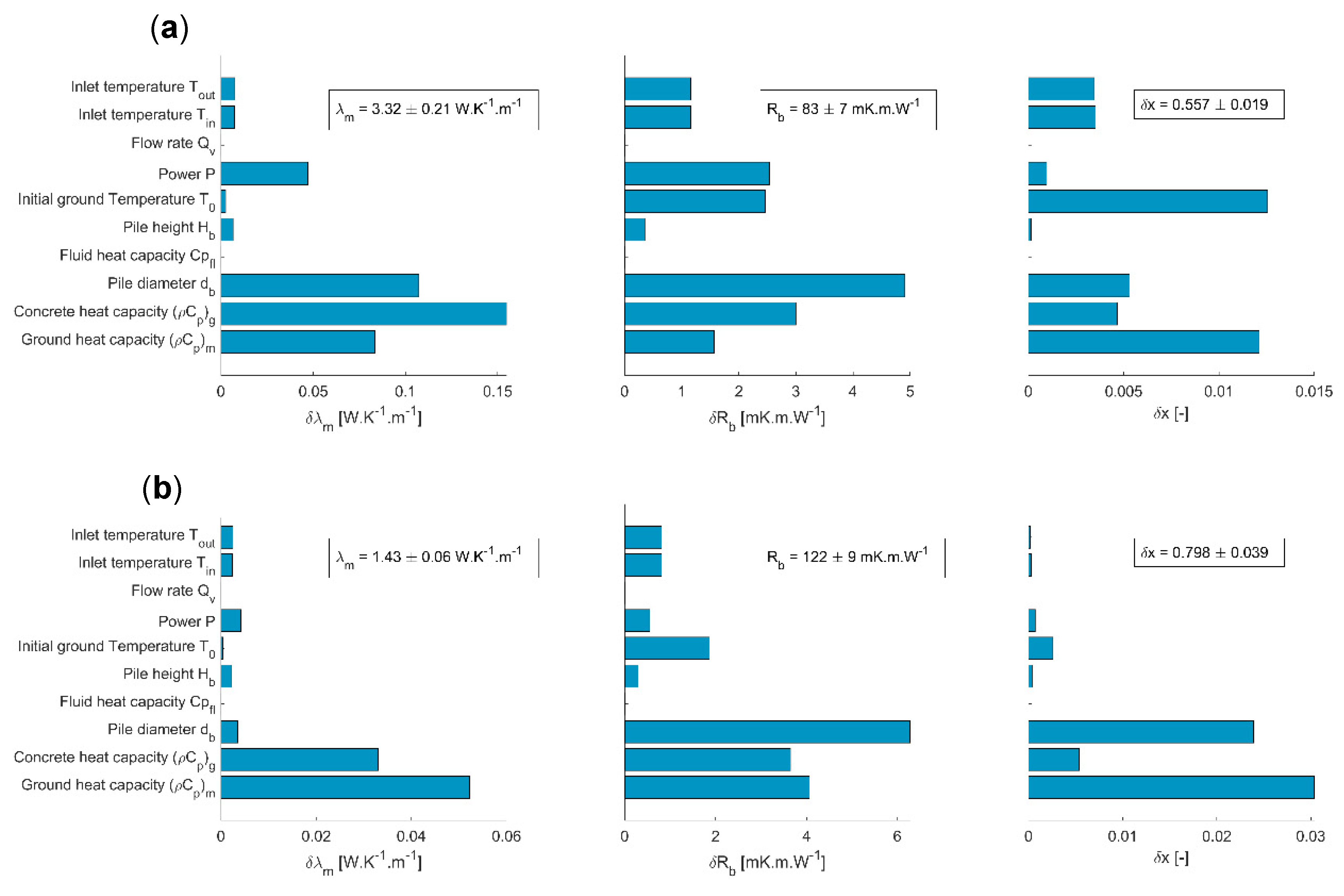
  • According to SIA standards, the volume-specific heat capacities of wet clay and wet sand are, respectively, in the range 2.0–2.8 MJ·K−1·m−3 and 2.2–2.8 MJ·K−1·m−3 [10]. We considered the error on the ground capacity as the half of these intervals, i.e., 0.3 MJ·K−1·m−3 for set B and 0.4 MJ·K−1·m−3 for set C. Typical ranges for concrete heat capacity could not be found in the literature, but given the values reported in previous studies [26,27], an error of 0.2 MJ·K−1·m−3 was chosen.
  • The error for the pile diameter and height were determined according to the UK specification for construction tolerances [28]. In this respect, it should be noted that the dimensions of a constructed pile should not be less than the specified dimensions. A tolerance on these dimensions of up to the lesser of 50 mm or 5% is permissible.
  • For set B, the test was performed with reference to the ASHRAE standard [29]. This states that the accuracy of temperature measurement must be less than 0.3 °C, for power measurements less than 2% and for flow rate measurements less than 5%. These are conservative values, since the test may have been performed with more accurate instruments.
  • For set C, the client specification had tighter accuracy requirements, which can be reasonably applied. They would be error for temperature of 0.1 °C, flow measurement of 0.01 m·s−1 and power to 5W.
For both datasets, the most significant sources of error are related to the heat capacities of the ground and the concrete (refer to Figure 8 which represent the distribution of X i y j Δ y j terms). As expected, temperatures and power play a more significant role for set B, where the standards are less restrictive. Errors on the pile diameter affect the inner parameters Rb and x significantly. The error on the ground thermal conductivity is 0.06 W·K−1·m−1 for set C (about 4%) and 0.20 W·K−1·m−1 for set B (about 6%) reflecting the more restrictive standards for set C. These values are well within the expected bounds for thermal response testing for boreholes, giving confidence to the new approach. For comparison, for a classical TRT on a BHE, Witte reported a typical error of 5% on the ground thermal conductivity [23].

3.2.2. Pile Thermal Capacity

The interest of the RC model on the resistive model is in the transitory phase. Here we arbitrarily define this phase as t* < 2.5, which results in 27 h for set B and 107 h for set C (Equation (2)). Once their inner parameters have been fitted, the classical and RC methods are compared in Figure 6. Given the similar results between the two methods in terms of conductivity prediction, for comparative purposes, the same input parameters are used in Figure 6. Note that both methods also use the normalized duration tmax* of experimental data, so tmax = 103 h for set B (tmax* ≈ 9.9) and tmax = 350 h for set C (tmax* ≈ 8.5). After 1 h of thermal load, the RC model overestimates the temperature of the fluid Tfl by only ≈1.0 °C for set B and ≈1.3 °C for set C. Beyond the transitory phase (t* > 2.5), the two approaches accord well with the measured temperature and both correctly forecast the measured temperature, especially when the t* > 5 criteria is reached. Further, the RC model allows an understanding of the dynamics of heat transfer within the pile (Figure 9). The pile is half-loaded at t* ≈ 0.4 for set B and t* ≈ 0.2 for set C.

4. Discussion and Recommendations

Whatever the interpretation method, the duration tmax for set C must be of the order of 250 h, i.e., about 10 days. This duration is not necessarily compatible with the management of a construction site. Therefore it is clear that the ground thermal conductivity may be obtained from a much shorter TRT carried out on a special purpose BHE as recommended by [17]. Yet this proposed approach retains a drawback, namely that the pile itself has not been characterized to allow appropriate forward simulation for the design process. No information has been obtained about its thermal resistance. While a closed form analytical expression has now been developed to obtain pile thermal resistance [30] this still requires information about concrete thermal conductivity and assumes accuracy of pipe placements compared with design.
Therefore we propose that by using the RC model the combination of a short BHE TRT and an additional short TRT on one of the constructed piles may provide the best solution. One TRT is performed on a BHE having a small radius (e.g., rb = 8 cm) to determine λm within a few days, while simultaneously a TRT is performed on the PHE to obtain the inner parameters for the RC model. This undertaking assumes that the ground is relatively homogeneous and lateral variations of composition and ground properties can be overlooked. This approach is illustrated with respect to datasets B and C. The best-fit values of λm are assumed to have been obtained independently from a BHE TRT. In this case values of 3.24 W/mK and 1.43 W/mK are used, respectively, for sets B and C, based on the results in Section 3. The RC model is then optimized for the pile TRT data with only two rather than three unknowns. The fitted values of x and Rb start to stabilize around tmax ≈ 30–40 h for set B at x ≈ 0.56–0.58 and Rb = 0.080 K·m·W−1 and tmax ≈ 100 h for set C at x ≈ 0.76–0.78 and Rb = 0.121–0.124 K·m·W−1 (Figure 10). For both datasets, the difference, with the value of Rb determined in Section 3, does not exceed 4%.
It is desirable to determine the minimum test duration tmax beyond which the determined values of Rb and x are reliable. Here we use as a criteria the ability of the RC model to forecast the evolution of the fluid temperature at the very end of the data record, from tmin’ to from tmax’. A second RMSE indicator ε’ is build considering tmin’ = 80 h and tmax’ = 100 h for set B, and tmin’ = 300 h and tmax’ = 350 h for set C. For set C, ε’ reaches a minimum around tmax* = 100 h (tmax* = 2.4), which suggests this duration is sufficient to estimate the temperature evolution from 300 to 350 h, as confirmed by the comparison to the recorded temperature (Figure 11).

5. Conclusions

A resistive-capacitive PHE model has been developed to capture the transient energy transfers within a pile. This model has been shown to perform well and in particular:
  • Numerical back-calculation of the model parameters on two thermal response tests yield similar values of ground conductivity and thermal resistance as the well-established infinite line source model.
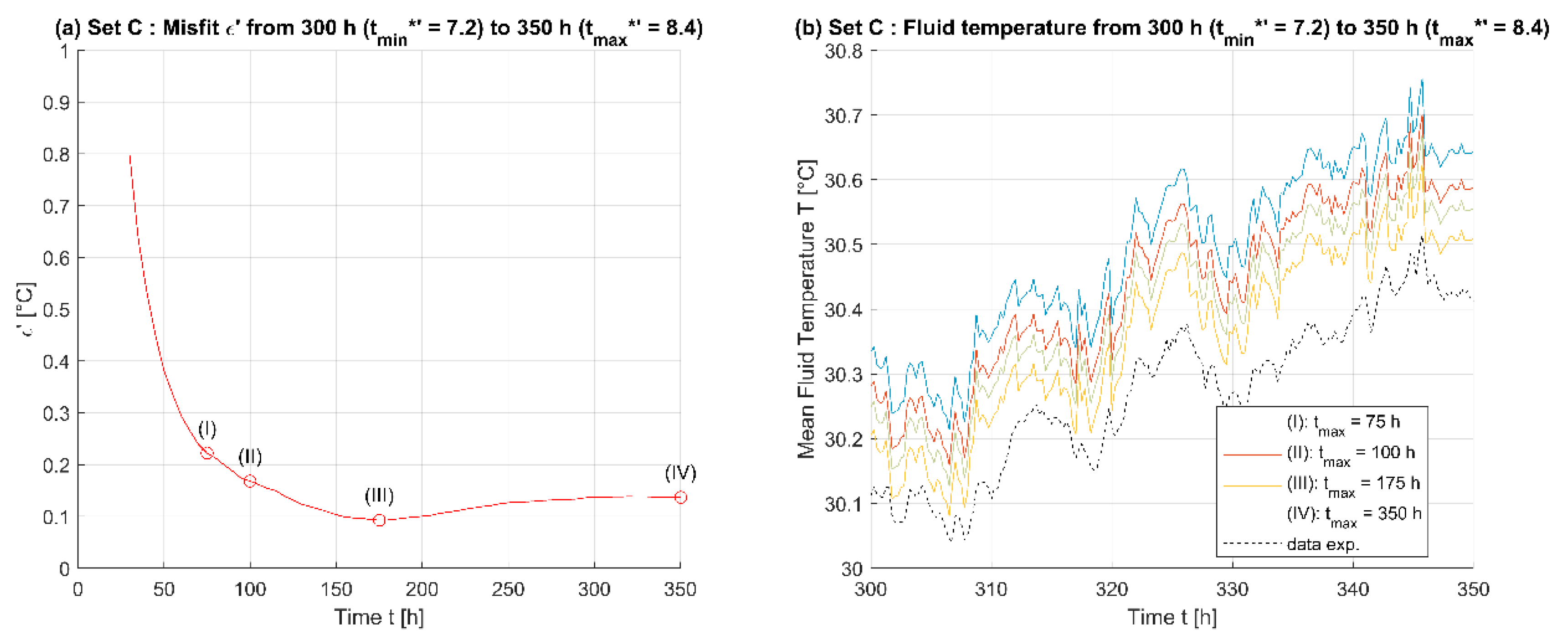
  • Inclusion of temporal superposition with the model allows reliable results to be obtained even when tests are affected by ambient air interference.
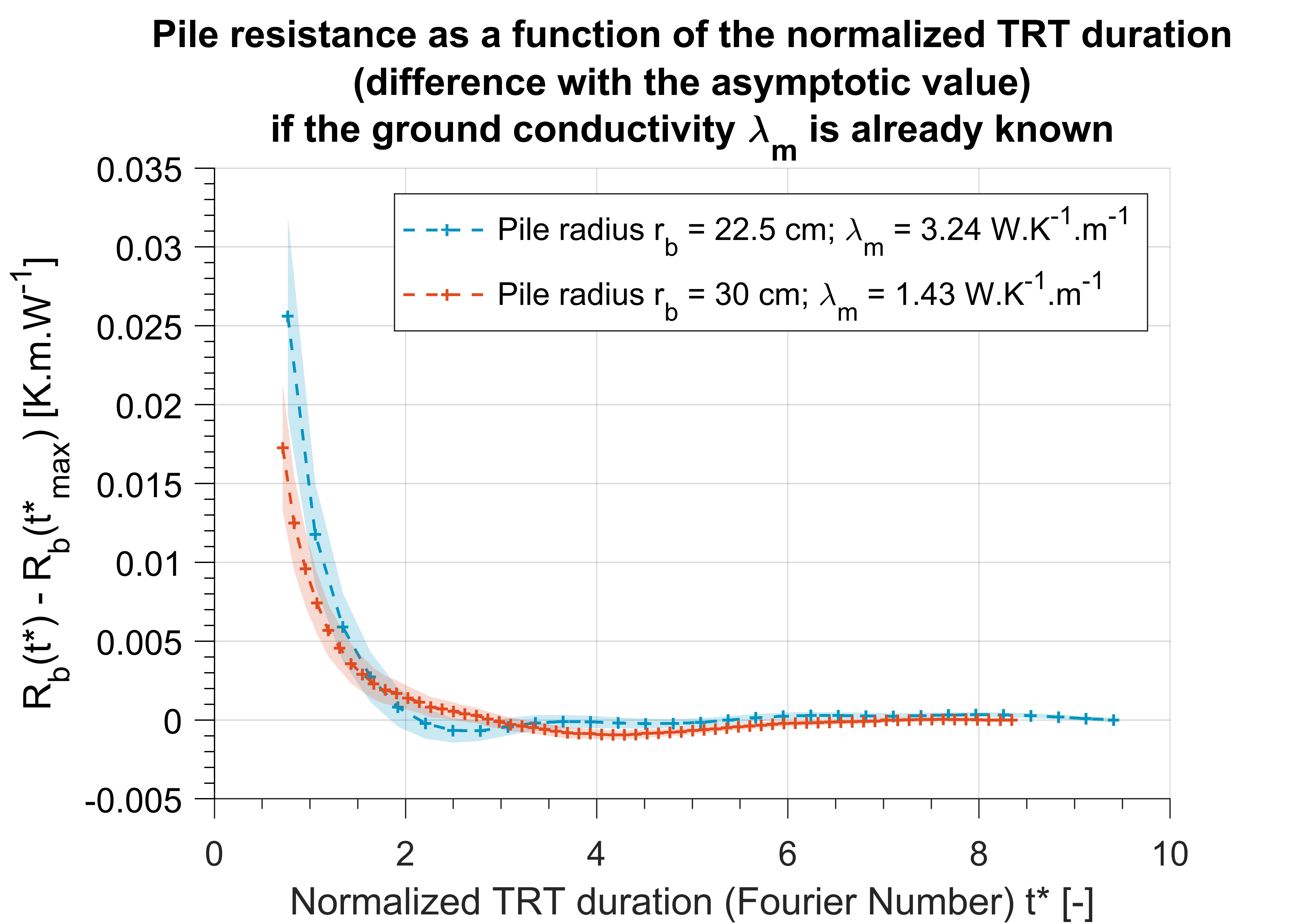
  • The RC model better represents the transient phase of pile warm-up in the early part of the test (approximately up to a Fourier number t* = 1 to 2).
  • The errors associated with the calculation of thermal conductivity are all less than 10% and well within expected ranges for boreholes thermal response tests interpreted with the classic infinite line source.
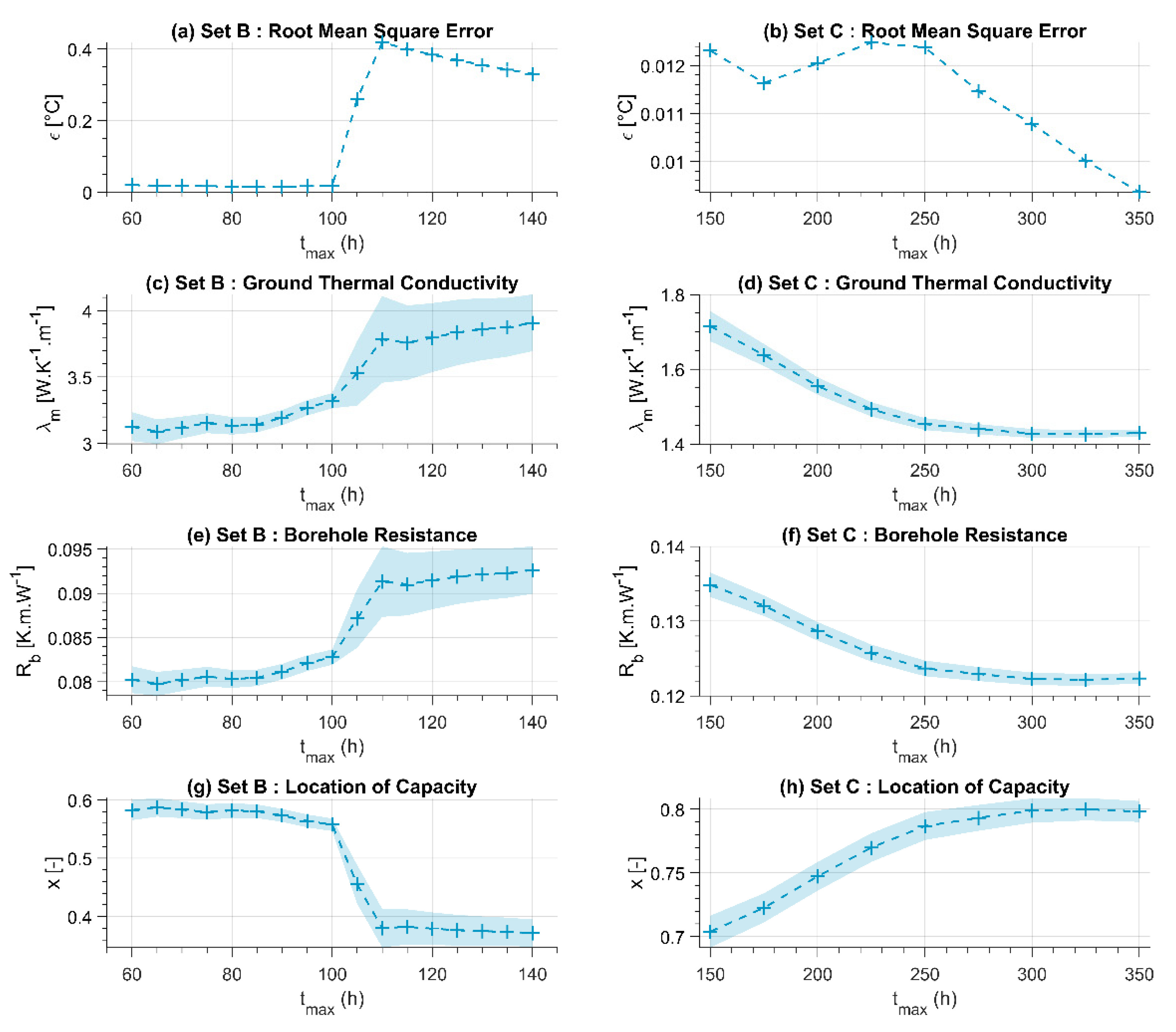
  • Standard back-calculation using the RC model does not allow to significantly reduce the TRT duration below t* = 5.
  • However, if the thermal conductivity can be obtained by another means, the time for the RC model to converge is much reduced meaning that pile resistance can be obtained from a pile TRT in a duration corresponding to a Fourier number t* ≈ 2 to 2.5.
Given these characteristics of the RC model the following novel approach for pile characterization is recommended:
  • Use a borehole at the same site and of the same length as the piles to carry out a BHE TRT to determine the effective soil thermal conductivity using the classical approach.
  • Carry out a short duration pile TRT according to Fourier number t* ≈ 2 to 2.5, or around 100 h for the cases demonstrated in this paper.
  • Interpret the pile TRT using the RC model to determine both the pile thermal resistance and the inner resistances of the RC model, which can then be used in forward simulation for design purposes.

Author Contributions

Conceptualization, C.M.; methodology, C.M.; software, C.M.; validation, C.M.; formal analysis, C.M.; resources, C.M. and F.L.; data curation, C.M. and F.L.; writing—original draft preparation, C.M.; writing—review and editing, C.M. and F.L.; visualization, C.M.; supervision, F.L.; project administration, C.M. and F.L. All authors have read and agreed to the published version of the manuscript.

Funding

The Exploitation of the RC Model for TRT Analysis was funded by the European Network for Shallow Geothermal Energy Applications in Buildings and Infrastructure COST-GABI, under reference “ECOST-STSM-TU1405-280216-071379 STSM”. Additionally, support from the Royal Academy of Engineering in the UK under their Research Fellow scheme is gratefully acknowledged.

Institutional Review Board Statement

Not applicable.

Informed Consent Statement

Not applicable.

Data Availability Statement

Not applicable.

Acknowledgments

Some of the TRT data used in this paper were provided by Crossrail, based on tests conducted by GI Energy. This project would not have been possible without their support.

Conflicts of Interest

The authors declare no conflict of interest.

Nomenclature

Latin Letters
athermal diffusivity [m·s−2]
C capacity of a node [J·K−1·m−1]
m ˙ flow rate [kg·s−1]
rradius [m]
Rthermal resistance [K·m·W−1]
ppower per meter of pile [W·m−1]
Ttemperature [°C]
ttime [s]
t*normalized time (Fourier number)
Greek Letters
εmisfit (root mean square error)
λthermal conductivity [W·K−1·m−1]
[ Λ ] conductance matrix [W·K−1·m−1]
ρCpvolume-specific heat capacity [J·K−1·m−3]
Subscripts
0undisturbed conditions
bborehole wall
cconcrete
flheat-carrier fluid
ininlet
mground
outoutlet
Superscripts
ntime step
*normalized value
Acronyms
BHEBorehole Heat Exchanger
CaRM Computational Capacity Resistance Model
DSTDuct Storage Model
GHEGround Heat Exchangers
GSHPGround-Source Heat Pumps
ICSInfinite Cylinder Source
ILS Infinite Line Source
PHEPile Heat Exchangers
RMSERoot Mean Square Error
SQPSequential Quadratic Programming

References

  1. Laloui, L.; di Donna, A. Energy Geostructures—Innovation in Underground Engineering; Wiley: Hoboken, NJ, USA, 2013. [Google Scholar]
  2. Brandl, H. Energy foundations and other thermo-active ground structures. Géotechnique 2006, 56, 81–122. [Google Scholar] [CrossRef]
  3. Pahud, D.; Hubbach, M. Measured thermal performances of the energy pile system of the dock midfield at Zürich Airport. In Proceedings of the European Geothermal Congress, Unterhaching, Germany, 30 May–1 June 2007. [Google Scholar]
  4. Angelotti, A.; Sterpi, D. On the performance of energy walls by monitoring assessment and numerical modelling: A case in Italy. Environ. Geotech. 2020, 7, 266–273. [Google Scholar] [CrossRef]
  5. Barla, M.; Di Donna, A.; Insana, A. A novel real-scale experimental prototype of energy tunnel. Tunn. Undergr. Space Technol. 2019, 87, 1–14. [Google Scholar] [CrossRef]
  6. Bidarmaghz, A.; Narsilio, G.A.; Johnston, I.W.; Colls, S. The importance of surface air temperature fluctuations on long-term performance of vertical ground heat exchangers. Géoméch. Energy Environ. 2016, 6, 35–44. [Google Scholar] [CrossRef]
  7. Han, C.; Bill, X. Feasibility of geothermal heat exchanger pile-based bridge deck snow melting system: A simulation based analysis. Renew. Energy 2017, 101, 214–224. [Google Scholar] [CrossRef] [Green Version]
  8. Alberdi-Pagola, M.; Poulsen, S.E.; Jensen, R.L.; Madsen, S. A case study of the sizing and optimisation of an energy pile foundation (Rosborg, Denmark). Renew. Energy 2020, 147, 2724–2735. [Google Scholar] [CrossRef]
  9. Gehlin, S. Thermal Response Test—Method, Development and Evaluation. Ph.D. Thesis, Luleå University of Technology, Luleå, Sweden, 2002. [Google Scholar]
  10. SIA. Norme Suisse. Sondes Géothermiques. SIA 384/6; Société Suisse des Ingénieurs et des Architectes: Zurich, Sweden, 2010. [Google Scholar]
  11. Loveridge, F.; Powrie, W.; Nicholson, D. Comparison of two different models for pile thermal response test interpretation. Acta Geotech. 2014, 9, 367–384. [Google Scholar] [CrossRef] [Green Version]
  12. Maragna, C.; Loveridge, F. A resistive-capacitive model of pile heat exchangers with an application to thermal response tests interpretation. Renew. Energy 2019, 138, 891–910. [Google Scholar] [CrossRef]
  13. Gehlin, S.; Hellström, G. Influence on thermal response test by groundwater flow in vertical fractures in hard rock. Renew. Energy 2003, 28, 2221–2238. [Google Scholar] [CrossRef]
  14. Zarrella, A.; Emmi, G.; Zecchin, R.; De Carli, M. An appropriate use of the thermal response test for the design of energy foundation piles with U-tube circuits. Energy Build. 2017, 134, 259–270. [Google Scholar] [CrossRef]
  15. Loveridge, F.; Olgun, C.G.; Brettmann, T.; Powrie, W. The Thermal Behaviour of Three Different Auger Pressure Grouted Piles Used as Heat Exchangers. Geotech. Geol. Eng. 2015, 33, 273–289. [Google Scholar] [CrossRef]
  16. Alberdi-Pagola, M.; Poulsen, S.E.; Loveridge, F.; Madsen, S.; Jensen, R.L. Comparing heat flow models for interpretation of precast quadratic pile heat exchanger thermal response tests. Energy 2018, 145, 721–733. [Google Scholar] [CrossRef]
  17. Jensen-Page, L.; Loveridge, F.; Narsilio, G.A. Thermal Response Testing of Large Diameter Energy Piles. Energies 2019, 12, 2700. [Google Scholar] [CrossRef] [Green Version]
  18. De Carli, M.; Tonon, M.; Zarrella, A.; Zecchin, R. A computational capacity resistance model (CaRM) for vertical ground-coupled heat exchangers. Renew. Energy 2010, 35, 1537–1550. [Google Scholar] [CrossRef]
  19. Brettmann, T.; Amis, T. Thermal Conductivity Evaluation of a Pile Group Using Geothermal Energy Piles. Geotech. Spec. Publ. 2011, 41165, 499–508. [Google Scholar]
  20. Carslaw, H.S.; Jaeger, J.C. Conduction of Heat in Solids; Clarendon Press: Oxford, UK, 1959. [Google Scholar]
  21. Eskilson, P. Thermal Analysis of Heat Extraction Boreholes; University of Lund: Sweden, Lund, 1987. [Google Scholar]
  22. Vieira, A.; Alberdi-Pagola, M.; Christodoulides, P.; Javed, S.; Loveridge, F.; Nguyen, F.; Cecinato, F.; Maranha, J.; Florides, G.; Prodan, I.; et al. Characterisation of ground thermal and thermo-mechanical behaviour for shallow geothermal energy applications. Energies 2017, 10, 2044. [Google Scholar] [CrossRef] [Green Version]
  23. Witte, H.J. Error analysis of thermal response tests. Appl. Energy 2013, 109, 302–311. [Google Scholar] [CrossRef]
  24. Bandos, T.V.; Montero, Á.; de Córdoba, P.F.; Urchueguía, J.F. Improving parameter estimates obtained from thermal response tests: Effect of ambient air temperature variations. Geothermics 2011, 40, 136–143. [Google Scholar] [CrossRef] [Green Version]
  25. Hellström, G. Duct Ground Heat Storage Model. Manual for Computer Code; Department of Mathematical Physics, University of Lund: Lund, Sweden, 1989. [Google Scholar]
  26. Suryatriyastuti, M.; Mroueh, H.; Burlon, S. Numerical analysis of a thermo-active pile under cyclic thermal loads. In Proceedings of the European Geothermal Conference (EGC 2013), Pisa, Italy, 3–7 June 2013. [Google Scholar]
  27. Gashti, E.H.N.; Uotinen, V.-M.; Kujala, K. Numerical modelling of thermal regimes in steel energy pile foundations: A case study. Energy Build. 2014, 69, 165–174. [Google Scholar] [CrossRef]
  28. Institution of Civil Engineers (Ed.) Specification requirements and guidance notes. In ICE Specification for Piling and Embedded Retaining Walls; Thomas Telford Ltd.: London, UK, 2016; pp. 21–216. [Google Scholar]
  29. ASHRAE. RP-1118. Investigation of Methods for Determining Soil and Rock Formation Thermal Properties from Short Term Field Tests; ASHRAE: Peachtree Corners, GA, USA, 2001. [Google Scholar]
  30. Claesson, J.; Javed, S. Explicit Multipole Formula for the Local Thermal Resistance in an Energy Pile—The Line-Source Approximation. Energies 2020, 13, 5445. [Google Scholar] [CrossRef]
Figure 1. Example of a pile heat exchanger following pile trimming and prior to connection to the building base slab and the ground-source heat pump system. In this particular case the heat transfer pipes are centrally located and still retain their protective sleeves, which were used to avoid their damage during trimming.
Energies 14 03375 g001
Figure 2. (a) Purely resistive classical model vs. (b) developed resistive-capacitive model.
Energies 14 03375 g002
Figure 3. Sketch of the piles used in the analysis: set B (left) and set C (right).
Energies 14 03375 g003
Figure 4. Evolution of the pile inlet (in) and outlet (out) temperatures for (a) set B and (b) set C; (c) set B and (d) set C as a function of the logarithmic elapsed time. In subplot (a) the dotted vertical lines enlighten the daily temperature variations.
Energies 14 03375 g004
Figure 5. Classical interpretation of TRT: values of ε, λm and Rb as a function of the duration of the integration tmax: misfit ε for (a) set B, (b) set C; λm for (c) set B, (d) set C, Rb for (e) set B, (f) set C. The stripe represents the 95% confidence interval on the fitted parameter.
Energies 14 03375 g005
Figure 6. Evolution of the experimental fluid temperatures, temperatures from the analytical approaches, TRNSYS DST model and the RC model for (a) set B (from 1 h to 100 h), (b) set C (from 1 h to 350 h).
Energies 14 03375 g006
Figure 7. Interpretation by the RC model: values of ε, λm and Rb and x as a function of the duration of the integration tmax: misfit ε for (a) set B, (b) set C; λm for (c) set B, (d) set C, Rb for (e) set B, (f) set C, x for (g) set B, (h) set C.
Energies 14 03375 g007
Figure 8. Sources of error (terms X i y j Δ y j in Equation (24)) for (a) set B and (b) set C.
Energies 14 03375 g008
Figure 9. Evolution of linear powers computed by the RC model: for (a) set B, (b) set C. pf: power given by the fluid, C d T C d t : transient power in the pile, pb: power at the borehole wall.
Energies 14 03375 g009
Figure 10. Interpretation of TRT with fixed λm: values of ε, Rb, x as a function of the duration of the integration tmax: misfit ε for (a) set B, (b) set C; Rb for (c) set B, (d) set C, x for (e) set B, (f) set C.
Energies 14 03375 g010
Figure 11. Set C: back-calculation of Rb and x with a fixed value of λm. (a) Evolution of the misfit ε’ with the duration of integration tmax. (b) Evolution of the temperatures from tmin’ to tmax’ for several values of tmax.
Energies 14 03375 g011
Table 1. Characteristics of the TRT.
Set BSet C
Depth of pile H [m]18.331.0
Radius of pile rb [m]0.2250.300
Geothermal equipmentDouble-U
(tested as single-U)
Double-U
External diameter of pipes [cm]3.002.50
Thickness of pipes [cm]0.290.23
Distance between two tubes diametrically opposed pipes [m]0.1570.425
Initial temperature of the ground T0 [°C]24.9714.23
Power applied P [kW]2.271.69
Linear power pf = P/H [W·m−1]123.754.6
Volume flow in the pile [m3·h−1]2.461.15
Duration of the heating [h]103.4354.1
Table 2. Considered values for the error on the input parameters.
Input ParameterError Values
Set BSet C
Ground heat capacity [MJ·K−1·m−3]0.40.3
Concrete heat capacity [MJ·K−1·m−3]0.20.2
Pile diameter [m]0.0250.03
Height of the equipped pile [m]0.050.05
Initial ground temperature [K]0.30.1
Fluid heat capacity [J·K−1·kg−1]1.09.5
Power [W]43.75.0
Flow rate [m3·s−1]3.44 × 10−53.29 × 10−6
Inlet temperature [K]0.30.1
Outlet temperature [K]0.30.1
Publisher’s Note: MDPI stays neutral with regard to jurisdictional claims in published maps and institutional affiliations.

