Evaluation of Building Energy Performance with Optimal Control of Movable Shading Device Integrated with PV System

Abstract

Among the envelope components (e.g., walls, roofs, floors, and windows, etc.) affecting the cooling and heating load of buildings, windows are the most thermally vulnerable. Shading devices can minimize the thermal load on windows due to solar radiation and decrease radiation effects. However, the load changes due to convection and conduction should be considered. Therefore, when a shading device is applied to a window, control logic for thermal blocking and heat retention is necessary to prevent the load changes. In addition, by combining the opposite features of photovoltaic (PV) that require solar radiation and the shading device to block solar radiation, energy-saving and production can be achieved simultaneously. Therefore, this study minimized the thermal effects of windows using a movable shading device integrated with PV and evaluated the PV power generation. This study evaluated the effects on window heat transfer by applying artificial intelligence techniques, which have recently attracted attention, to system operation. To achieve this, artificial neural network (ANN)-based control logic was developed, and the control performance of the system was assessed using simulations. In ANN control, the window heat transfer was 86.3% lower in a cooling period and 9.7% lower in a heating period compared with that of a shading device fixed at 45°. Furthermore, the PV system produced 3.0 to 3.1% more electric power under optimal control during the cooling period.

1. Introduction

Industrialization has resulted in the emission of considerable amounts of greenhouse gases. Accordingly, environmental and energy-related issues (e.g., global warming, climate change) have arisen. In this context, the United Nations (UN) enacted a Framework Convention on Climate Change in 1988 to address global warming and climate change. This Framework Convention on Climate Change was signed as a formal agreement having legal-binding power on five occasions from 1997 to 2015 [1].

To respond to climate change, the government of South Korea also enacted the Framework Act on Low Carbon, Green Growth in 2010 [2]. Moreover, the government of South Korea submitted to the UN a greenhouse gas-reduction target of 37% compared to business as usual. One hundred ninety-five countries, which account for more than 90% of greenhouse gas emissions, are making various efforts to respond to a rapidly changing climate. In 2017, the greenhouse gas emissions (615.8 million tons CO_2eq) in the energy sector of South Korea accounted for approximately 86.8% of the total greenhouse gas emissions [3]. To meet the greenhouse gas-reduction target, efficient usage and reduced energy use are needed. The annual total energy demand of South Korea is accounted for mainly by industry (55%), buildings (24%), and transportation (21%) [4]. Among these sectors, energy demand in the building sector is continuously increasing as the residential environment, and standard of living improves. Thus, the energy used by the continuously increasing number of buildings must be reduced. Moreover, zero-energy buildings, building energy efficiency, and green buildings are receiving increasing attention as part of the effort to reduce energy demand by buildings [5].

Among the various factors affecting the building energy use, windows are the most thermally vulnerable, and thus, the fluctuations in building energy use due to heat loss/gain through windows are significant to maintain desired room temperatures. Therefore, suitable shading devices on windows are needed to reduce building energy use [6]. Shading devices are typically classified as internal or external devices. Furthermore, the effect of a shading device on building energy use depends on the shape and type of the device. External shading devices can prevent solar radiation from entering the building. Thus, it can decrease the fluctuations in building energy use more effectively than internal shading devices. External shading devices are typically used to minimize the effects of solar radiation. However, the use of a shading device affects not only heat transfer by radiation but also heat transfer by convection and conduction. Therefore, integrated analyses, including convection, conduction, and radiation heat transfer, can clarify the effect on building energy use.

To this end, in this study, we developed a movable shading device integrated with a photovoltaic (PV) system and applied it to a window, the most vulnerable component. This system combines the most widely-used passive method and renewable energy. Moreover, because it is a relatively simple system, it can be applied regardless of the building size and purpose. The developed system was materialized using a building energy simulation.

2. Previous Evaluations of Energy Performance of Buildings with Shading Devices

Shading devices are typically classified as internal or external devices, and their effect on building energy use depends on their type. Therefore, we conducted a literature review of studies on various shading devices.

Table 1. Literature related to various shading devices.

Reference Number	Year	Objective	Location	Methodology		Calculation Model	Analysis Parameters
				Experiment	Simulation
[7]	2010	Evaluation of building energy performance	Mexico City, Mexico Cairo, Egypt Lisbon, Portugal Madrid, Spain London, UK	×	○	TRNSY type 56	Cooling energy Heating energy
[8]	2013	Evaluation of building energy performance	Palermo, Rome, and Milan, Italy	×	○	EnergyPlus	Cooling energy Heating energy
[9]	2014	Evaluation of building energy performance	Chania and Athens, Greece	○	○	Ecotect, EnergyPlus	Energy production PV power generation
[10]	2014	Evaluation of building energy performance	Seoul, Korea	○	×	Measurement	PV power generation, illuminance Lighting energy
[11]	2015	Evaluation of wall thermal performance	Hefei, China	○	○	Previous algorithm	Air massflow rate Outdoor temperature
[12]	2017	Evaluation of building energy performance	Hong Kong, China	○	○	EnergyPlus	PV power generation
[13]	2017	Evaluation of building energy performance	Seoul, Korea	○	×	Measurement	PV power generation Illuminance
[14]	2018	Evaluation of building energy performance	Seoul, Korea	○	×	Measurement	Cooling energy Heating energy Lighting energy PV power generation, illuminance

shows the previous studies of shading devices.

Palmero-Marrero and Oliveira [7] analyzed the effect of louver-type shading devices attached to the eastern, western, and southern façades of a building on the building energy requirements. The evaluation was conducted in five cities (Mexico City, Cairo, Lisbon, Madrid, and London) at different latitudes using a TRNSYS simulation. The results indicated that in Cairo, Lisbon, and Madrid, the cooling and heating energy demand was lower when the louver-type shading device was installed than when it was not installed (Cairo: 55–60%, Lisbon: 38–50%, Madrid: 3–9%). By contrast, the heating energy demand increased in Mexico and London.

Bellia et al. [8] analyzed the effect of shading device installation on building energy use in Italian climates. The results showed that the building energy use was reduced by 20%, 15% and 8% in Palermo (the hottest climate), Rome (intermediate climate), and Milan (the coldest climate), respectively, when the shading device was installed compared to when it was not installed. In cold winter climates, the heating energy requirements are higher than the cooling energy requirements, and thus the energy savings were lower.

Mandalaki et al. [9] assessed the energy production of PV modules integrated with typical shading devices in an office building in Greece by conducting a simulation using Ecotect and EnergyPlus. The PV energy production measured in Athens and Chania was found to be similar to the simulation results. The difference between the measurement results and simulation results was 9–11%.

Kim et al. [10] evaluated the energy performance of a building with PV blind control. The PV blind slat angle was set according to the season (February, May, June, and August) and time (09:00–18:00). The results showed that when the slat angle of the PV blind was controlled, the PV blind generated 32% more electric power and reduced building energy use by 35%.

Hong et al. [11] evaluated the thermal performance of a Trombe wall using a Venetian blind by conducting a three-dimensional simulation. The results indicated that the heat-collecting efficiency of the Trombe wall with Venetian blind use increased in winter, and the wall prevented overheating in summer.

Zhang et al. [12] assessed the potential benefits of the use of PV shading devices in Hong Kong using simulations based on EnergyPlus. The results indicated that the installation of a PV shading device on a southwestern window reduced energy use by up to 69.16 kWh/m² annually. Moreover, the maximum energy reduction compared to the window with no shading device was 45.7%.

Hong et al. [13] developed an optimal control method to block direct sunlight inflow and produce electric power using PV shading devices on a Venetian blind and roll screen. Under optimal control, the interior illuminance of the Venetian blind was 1.6–1.9 times higher than that of the roll screen. The Venetian blind showed superior performance in the indoor lighting environment. However, the electric power generation of the Venetian blind was 3.96–14.32% that of the roll screen.

Hong et al. [14] analyzed the effect of bidirectional PV blind control on the energy use of a mock-up room. Tests were conducted by manufacturing a reference room and a test room. The results indicated that bidirectional PV blind control was more effective for energy saving than unidirectional PV blind control. The lighting energy was reduced by 4.62–35.50%, and the heating energy decreased by 2.10–11.46%.

As discussed above, numerous studies have evaluated the energy performance of buildings with various shading devices (Table 1), including fixed and flexible shading devices. In a few studies, an optimal control method was combined with a flexible device, and the building energy use was reduced. Shading devices are indispensable for reducing building energy use. Because shading devices are used on windows, it is very important to evaluate the thermal performance of windows when shading devices are applied. Moreover, because the window is the most thermally vulnerable building structure, its effect on building energy use is significant. Therefore, it is necessary to evaluate the thermal performance of a window with a shading device. However, in most previous studies, the window thermal performance did not receive sufficient attention. The previous studies were limited to evaluating the effect of shading devices on building energy simply. Of course, it is important to evaluate the effects of the application of shading devices on building energy, but in the end, these effects are caused by window heat transfer. In particular, heat transfer is one of the important indicators for evaluating the thermal performance of windows. In addition, the window heat transfer is affected by conduction, convection, and radiation depending on time and season. Therefore, this study evaluated the effect of a shading device on window heat transfer. In this study, the shading device was optimally controlled to minimize the changes in the window heat transfer by operating the shading device. This study evaluated was not only the window heat transfer according to the optimal control but also the amount of additional power generated by the attached PV. In addition, this system was differentiated from previous studies and applied automated artificial intelligence control logic rather than manual control or fixed shading device. Furthermore, this study predicted the window heat transfer in advance and controlled the shading device; it could be effectively responded to building energy.

3. Research Process

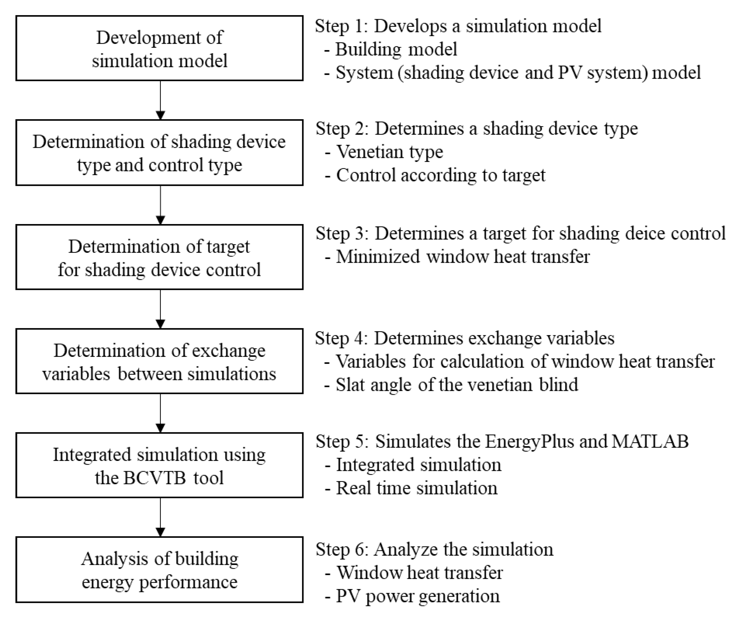
This research was conducted as follows: (1) development of simulation model; (2) determination of shading device type and control type; (3) determination of target for shading device control; (4) determination of exchange variables between simulations; (5) integrated simulation using the BCVTB tool; and (6) analysis of building energy performance (Figure 1).

The first step was to model the building and system. The target building for the simulation is a virtual residential building; it was modeled according to the US residential building standard code of the 2009 International Energy Conservation Code (IECC) [15]. The shading device is installed on a southern window of the target building, and the PV system attached to the shading device (efficiency: 15.89%) was modeled as a polycrystalline silicon panel.

The second step was the determination of the type of shading device and control. An external Venetian shading device was used, and the building energy performance under slat angle control was assessed.

The third step was the determination of the control target for the shading device. The proposed system was operated to minimize the changes in heat transfer at the window, which is the most thermally vulnerable building component.

The fourth step was the determination of the exchange variables between simulations. EnergyPlus [16] and MATLAB [17] were used in this study, and the slat angle was selected as the exchange variable. During the simulation, the slat angle was exchanged in real time to minimize the change in window heat transfer.

The fifth step was the materialization of the integrated simulation. In this study, we connected EnergyPlus and MATLAB using the Building Controls Virtual Test Bed (BCVTB) [18] and materialized an integrated simulation that enabled real-time control.

The sixth step was simulation analysis. This study analyzed the window heat transfer on the basis of the results and evaluated the building energy performance in terms of the electric power generated by the attached PV.

4. Methodology

This study materialized a movable shading device integrated with the PV and assessed the building energy performance after installation and operation. Moreover, this study used a sequence consisting of simulation modeling, optimal control model development, and integrated simulation. The methodology is described below.

4.1. Simulation Tools

Three simulation tools (EnergyPlus (Ver. 8.5), MATLAB (Ver. 2016a), and BCVTB (ver. 1.6.0)) were used to evaluate the energy performance of a building using the developed system.

EnergyPlus is a representative building energy simulation tool developed by the US Department of Energy (DOE). It was developed by combining the advantages of the DOE-2 and BLAST programs, and it enables dynamic heat transfer analysis because it uses a heat balance algorithm recommended by the American Society of Heating, Refrigerating and Air-Conditioning Engineers (ASHRAE). Therefore, EnergyPlus was used to analyze window heat transfer and to model the simulation target building and the system.

MATLAB is a numerical analysis and programming software developed by MathWorks in the US. It uses C and Fortran as programming languages and uses matrix calculations. MATLAB is used for data analysis, algorithm development, numerical analysis, programming, and prediction model development. With increasing interest in artificial intelligence in recent years, it is being used as a software to materialize machine learning, reinforcement learning, and deep learning. In this study, it was used to develop an optimal control model based on artificial intelligence for a movable shading device integrated with the PV.

The BCVTB is a program that can build an integrated simulation by interlocking two or more programs or software packages. Its operation is based on Ptolemy II, and it enables the exchange of variables between interlocked programs. The simulation tools that can typically be interlocked include EnergyPlus, MATLAB, Simulink, Radiance, ESP-r, and TRNSYS. This study conducted the integrated simulation by interlocking EnergyPlus and MATLAB using BCVTB.

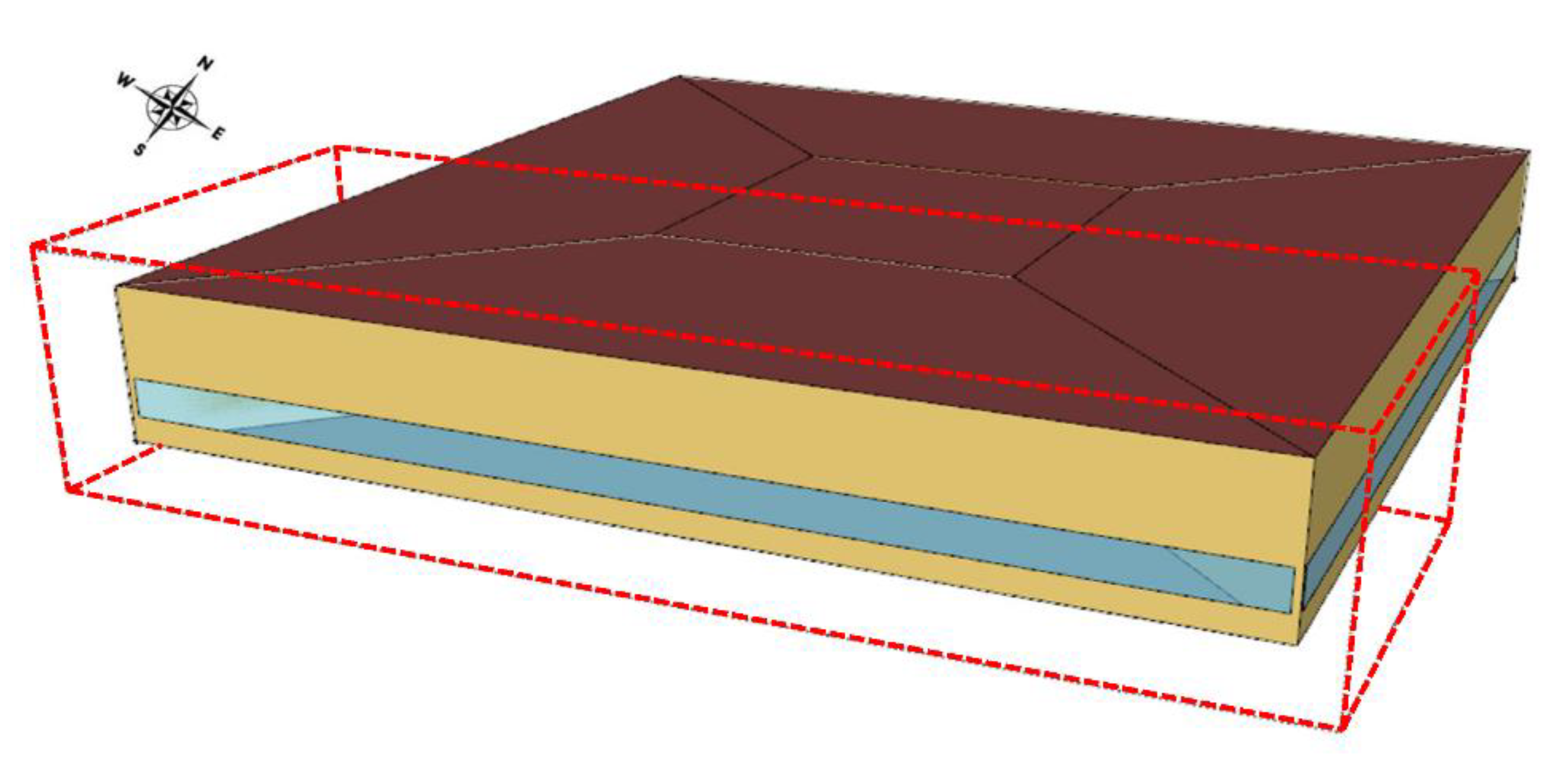
4.2. Model for Building Energy Simulation

This study modeled the target building and system for the simulation. A virtual residential building located in Daejeon was used as the simulation target building. The building had a square shape, which made it possible to analyze the thermal characteristics from all orientations. The building area was set to 232 m² (2500 ft²), the average area of a residential building in the US. The building envelope material properties were selected according to the 2009 IECC design standard for residential buildings in the US. A window-to-wall ratio (WWR) of 24.67% was obtained by converting the window-to-floor ratio of the 2009 IECC code to the WWR. The window was a 6 mm thick single window. Figure 2 shows the simulation target building; the analysis was conducted only on the control volume (i.e., south zone), which is enclosed by a red dotted line.

Table 2. Window input variables.

Parameter	Value
Optical data type	Spectral average
Solar transmittance at normal incidence	0.837
Front side solar reflectance at normal incidence	0.075
Back side solar reflectance at normal incidence	0.075
Visible transmittance at normal incidence	0.898
Front side visible reflectance at normal incidence	0.081
Back side visible reflectance at normal incidence	0.081
Front side infrared hemispherical emissivity	0.840
Back side infrared hemispherical emissivity	0.840
Conductivity	0.900 W/m·K
Thickness	0.006 m

presents the major input variables of the window.

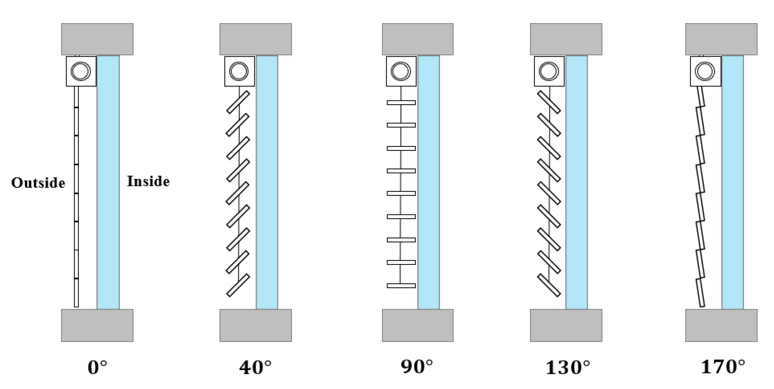
The movable shading device integrated with the PV proposed in this study used the Venetian blind with a controllable slat angle. This system is installed on the external part of a south zone window. The slat angle is controlled to be within 0° and 170° at 10° intervals (because 180° has the same shape as 0°, it was excluded). Figure 3 shows the shape of the movable shading device integrated with the PV with different slat angles, and

Table 3. Shading device input variables.

Parameter	Value
Slat operation	Horizontal
Slat width	0.048 m
Slat separation	0.048 m
Slat thickness	0.002 m
Slat angle	0°–170°
Slat conductivity	0.900 W/m·K
Front side slat beam solar reflectance	0.700
Back side slat beam solar reflectance	0.700
Front side slat diffuse solar reflectance	0.700
Back side slat diffuse solar reflectance	0.700
Slat beam visible transmittance	0.000

lists the major input variables.

Table 4. Electrical characteristics of the PV module.

Parameter	Value
Rated power	310 W
Voltage at Pmax	36.3 V
Current at Pmax	8.54 A
Warranted minimum Pmax	310 W
Short-circuit current (Isc)	8.96 A
Open-circuit current (Voc)	45.4 V
Module efficiency	15.89%
Operating module temperature	−40 °C–+85 °C
Maximum system voltage	1000 V (IEC)
Maximum series fuse rating	15 A
Maximum reverse current	20.25 A
Power tolerance	0–+5 W

shows the performance of the PV module integrated with the movable shading device.

4.3. Development of Optimal Control Model

This study aimed to develop an optimal control model based on artificial intelligence using the neural networks toolbox in MATLAB. The artificial neural network (ANN) was used as the artificial intelligence technique. Because ANN is more responsive to external changes than mathematical control models, its predictions are more accurate. The optimal control model was learned using the Levenberg–Marquart algorithm, which has the advantages of rapid learning and low memory usage by the software [19]. The proposed movable shading device integrated with the PV is controlled to minimize the changes in window heat transfer. Two optimal control models, i.e., a cooling period control model and a heating period control model, were developed. The dataset was constructed using EnergyPlus simulation data. During this process, EnergyPlus simulation used the Daejeon weather data from International Weather Files for Energy Calculations 2.0 [20]. This dataset used August data for the cooling period and January data for the heating period because, in Daejeon, the maximum cooling load and heating load occur in August and January, respectively. Data for every 10 min were used, and 70%, 15%, and 15% of the dataset was used for training, validation, and testing, respectively.

Table 5. Dataset parameters and value ranges.

Parameter	Value
	Cooling Period	Heating Period
Outdoor air temperature (°C)	17.0–36.0	−20.0–10.8
Indoor air temperature (°C)	19.6–26.0	20–25.4
Surface outside face temperature (°C)	18.3–33.4	−1.4–21.3
Surface inside face temperature (°C)	15.8–42.8	−16.9–28.8
Incident solar radiation (W/m2)	0.0–495.2	0.0–896.3
Net window heat transfer (W)	0.0–2582.3	0.1–5295.1
Slat angle (°)	0–170

shows the ranges of values in the dataset.

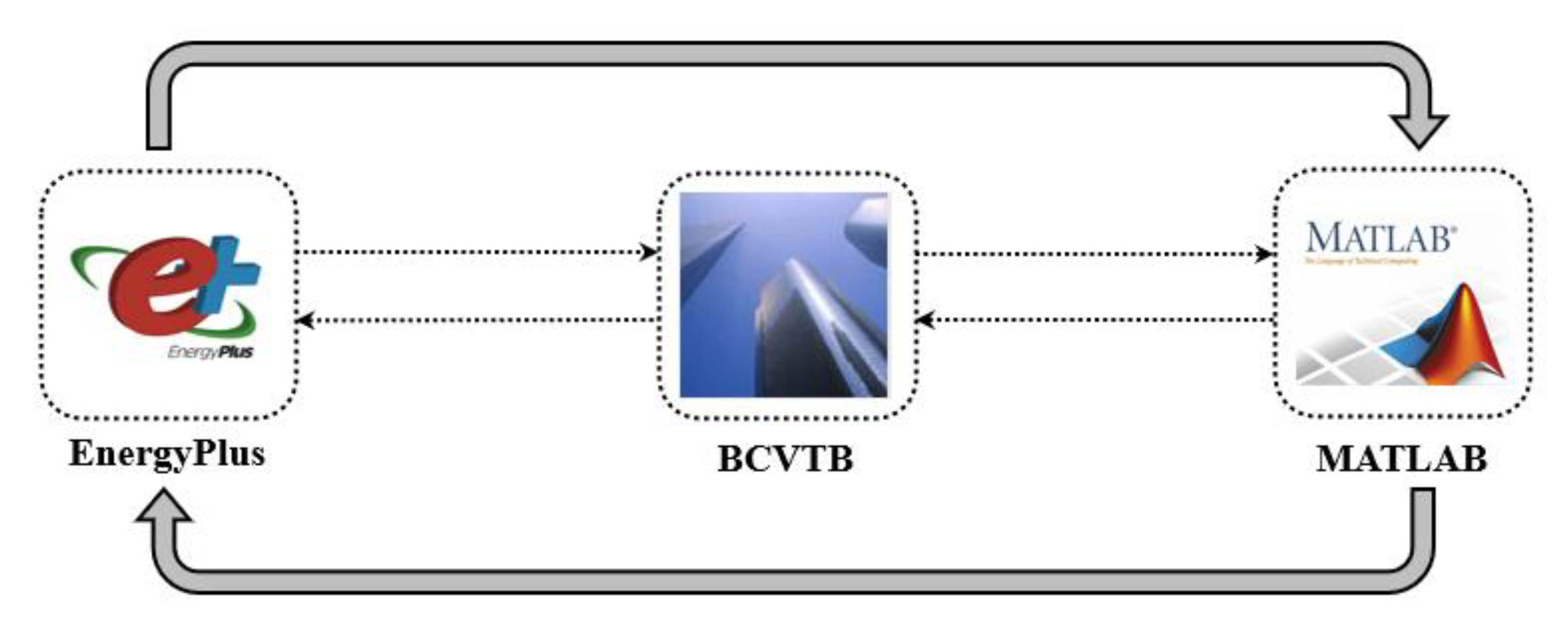
4.4. Integrated Simulation

This study conducted an integrated simulation of the control of the movable shading device integrated with the PV. EnergyPlus and MATLAB were interlocked using BCVTB, and real-time control was enabled by determining the exchange variables between the simulations.

Table 6. Exchange variables between EnergyPlus and MATLAB.

EnergyPlus to MATLAB	MATLAB to EnergyPlus
Outdoor air temperature (°C)	Slat angle (°)
Indoor air temperature (°C)
Surface outside face temperature (°C)
Surface inside face temperature (°C)
Incident solar radiation (W/m2)

presents the exchange variables between EnergyPlus and MATLAB.

The integrated simulation was conducted as follows: (1) EnergyPlus delivers five variables for the window heat transfer calculation to MATLAB. (2) MATLAB predicts the minimum value of the window heat transfer using the variables from EnergyPlus. (3) MATLAB delivers the slat angle at the minimum window heat transfer to EnergyPlus. (4) EnergyPlus again transfers to MATLAB five variables for the next timestep calculated using the slat angle from MATLAB. The integrated simulation was conducted by repeating these steps. Figure 4 shows a simplified conceptual diagram of the integrated simulation.

5. Results of ANN Model

This section explains the development of the ANN-based optimal control model. This model used min–max normalization to apply the input data for learning on the same scale. This study normalized the data to values between 0.1 and 0.9 to prevent the generation of values of 0 and 1 [21], which could adversely affect the calculation of the window heat transfer. The min–max normalization algorithm is shown in Equation (1).

$$X_{new}=\left(\frac{X-\min \left(X\right)}{\max \left(X\right)-\min \left(X\right)}\right)\times 0.8+0.1$$

(1)

where $X_{new}$ is the normalized data, $\mathrm{X}$ is the existing data, $\min \left(X\right)$ is the minimum value of the existing data, and $\max \left(X\right)$ is the maximum value of the existing data.

Furthermore, the optimal control model used the coefficient of variance of the root-mean-squared error (cvRMSE) to evaluate the accuracy of the ANN model and the integrated simulation. Equations (2) and (3) outline the RMSE and cvRMSE calculations.

$$RMSE=\sqrt{\frac{{\displaystyle \sum }{\left(S-M\right)}^2{}_{interval}}{N_{interval}}}$$

(2)

$$cvRMSE=\frac{RMS{E}_{period}}{A_{period}}$$

(3)

where $S$ is the predicted data (MATLAB data), $M$ is the measured data (EnergyPlus data), $N_{interval}$ is the number of measured data points, and $A_{period}$ is the average measurement period. The optimal control model performs a validation process. The model was validated after the accuracy of the ANN model, and integrated simulations were assessed. Finally, we evaluated the building energy performance using the optimal control model and analyzed the corresponding power generation of the PV system.

5.1. Development of ANN Model

This study developed an optimal control model using the dataset. The model was composed of 15 hidden neurons and 1 hidden layer. The learning rate and momentum constant of this model were set to 0.3. Each variable was set based on the work of Moon et al. [22]. The input data consist of outdoor air temperature, indoor air temperature, surface outside face temperature, surface inside face temperature, incident solar radiation, and slat angle, and the output was the net window heat transfer. According to an analysis of the accuracy of the ANN-based optimal control model, the cvRMSE was approximately 9.9% and 9.8% for the cooling period and heating period, respectively.

5.2. Validation of ANN Model

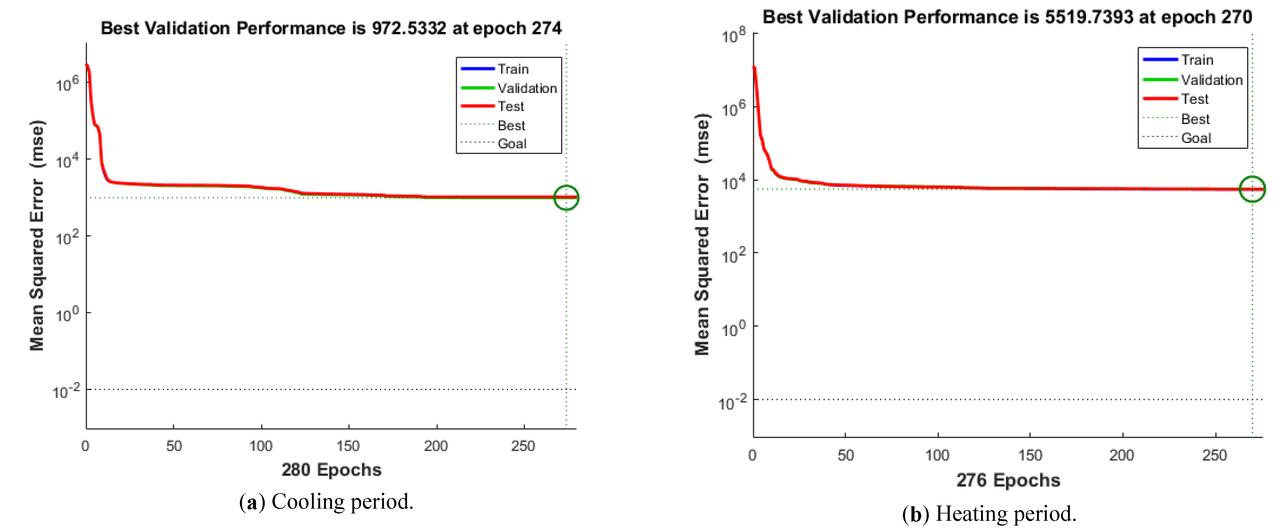
The model was validated to determine its applicability. To evaluate the applicability, the output value and error of the training, validation, and test datasets were identified. Figure 5 presents the mean squared error (MSE). The x-axis (MSE) represents the error, and the y-axis (Epochs) indicates the time point at which the repetitive training was suspended.

According to the error analysis, the model predictions showed the best validation performance after 274 and 270 repetitions for the cooling and heating periods, respectively. Moreover, the error characteristics of the training, validation, and test datasets showed a similar pattern. The results showed that the optimal control model was highly accurate.

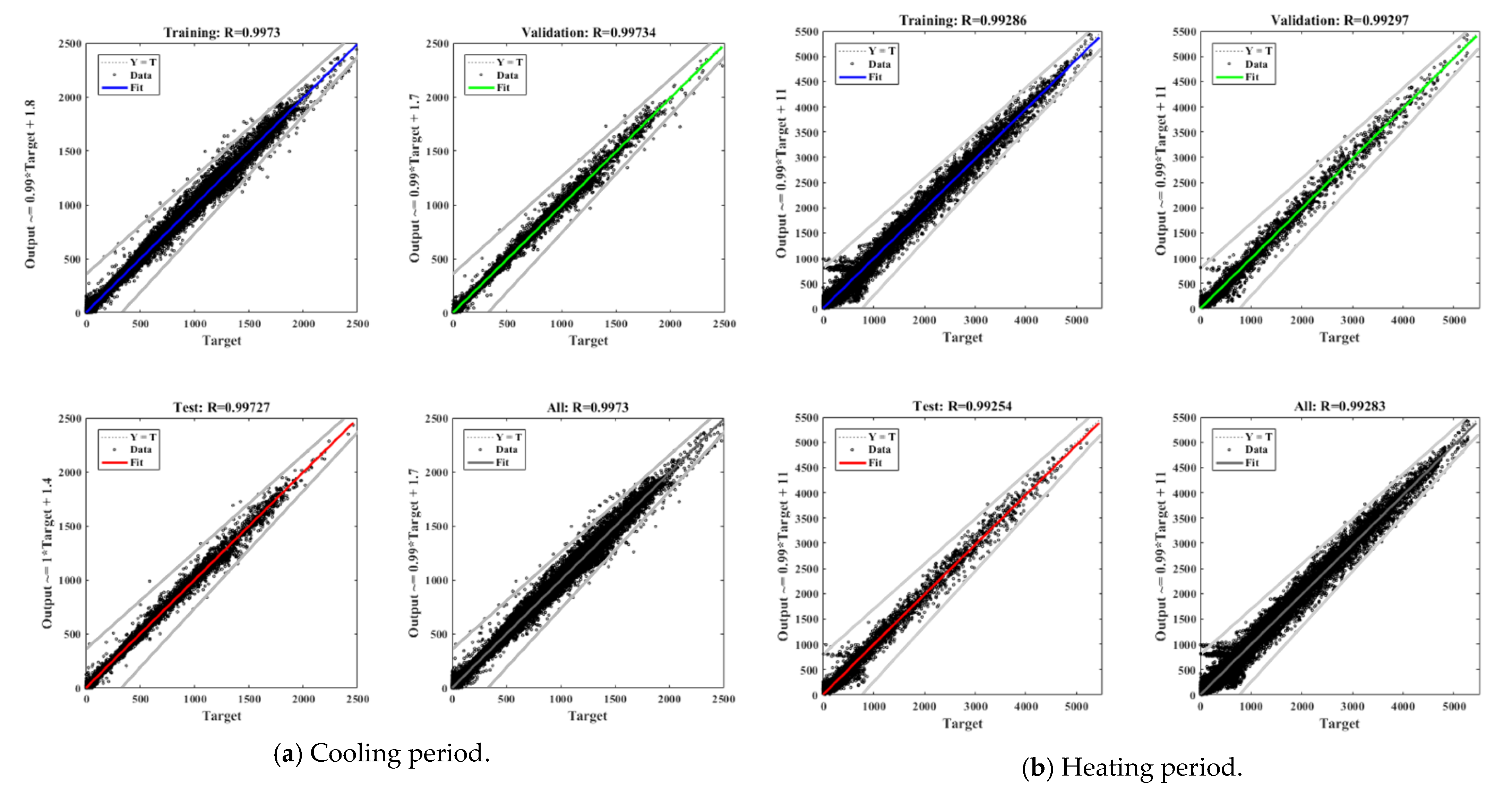
Figure 6 presents the regression analysis of the optimal control model. The target on the x-axis is the dataset, and the output on the y-axis is the ANN output value. In addition, this study evaluates the accuracy between target values and output values. The gray line is 10% of the deviation line.

Most of the data values were distributed within 10% of the deviation line. According to the regression analysis results, the R² values of the training, validation, and test datasets and the total were greater than 0.99. Most of the data values were distributed within 10% of the deviation line. In addition, the mean absolute percentage error (MAPE) values for regression results for the cooling and heating seasons were about 4.89% and 9.40%, respectively. This result suggests that the ANN-based optimal control model could make highly accurate predictions during the operation of the integrated simulation.

6. Results and Discussion

In this section, this study evaluated the building energy performance using ANN-based optimal control of the movable shading device. To this end, the window heat transfer and PV power generation are analyzed. To determine the window heat transfer, the conduction, convection, and radiation were analyzed. Moreover, during the window heat transfer analysis, cases with and without optimal control were considered, and the characteristics in daytime and nighttime were also compared. During this period, the day with the highest outdoor temperature (9–10 August) in the cooling period and the day with the lowest outdoor temperature (23–24 January) in the heating period were selected for the analysis of different times. Daytime and nighttime were defined as times with solar radiation (10:00–17:00) and without solar radiation (00:00–03:00, 20:00–23:00), respectively, and the data for 8 h were analyzed for both cases. 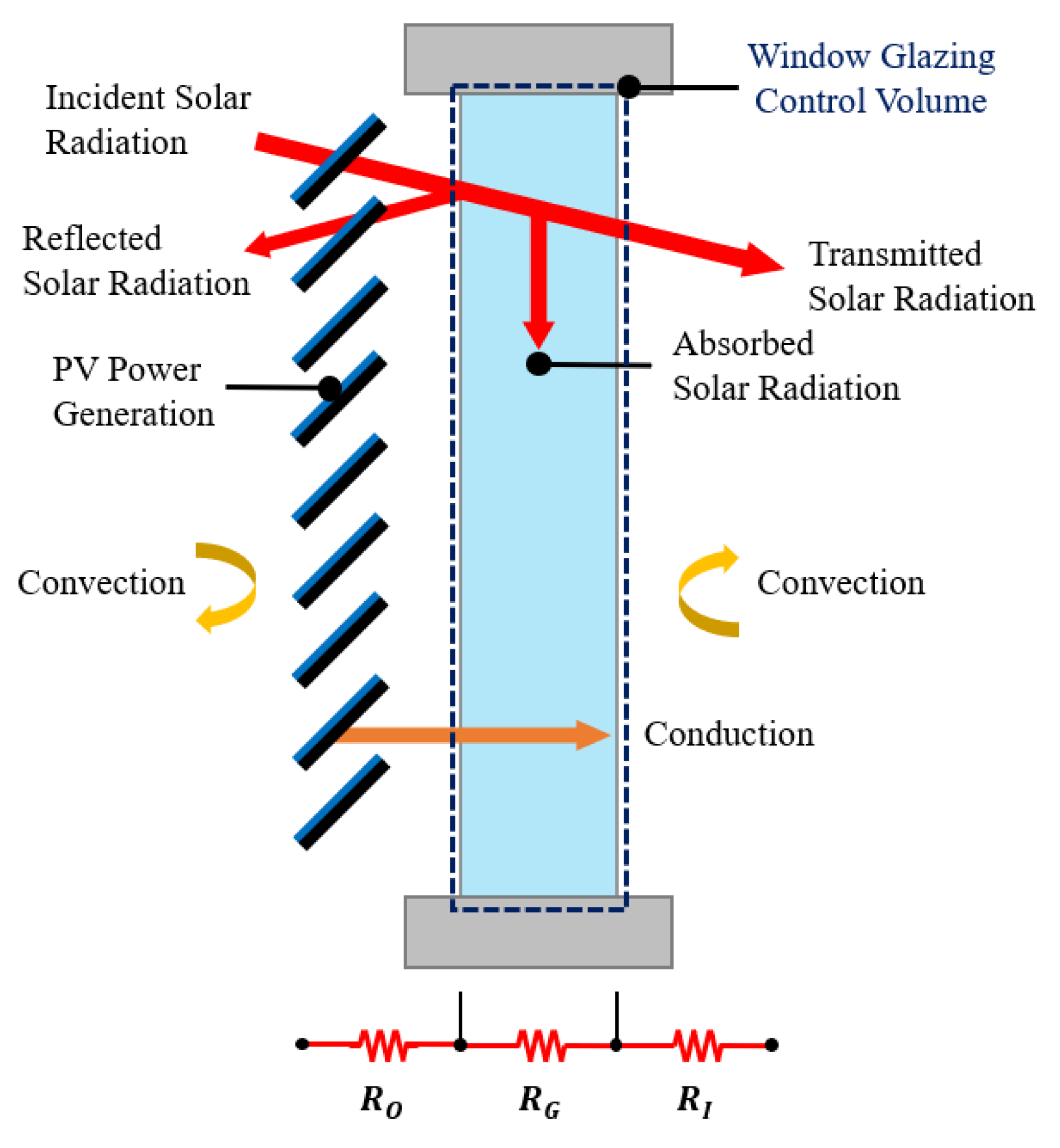Figure 7 shows a simplified diagram of window heat transfer and PV power generation.

6.1. Performance of the Integrated Simulation

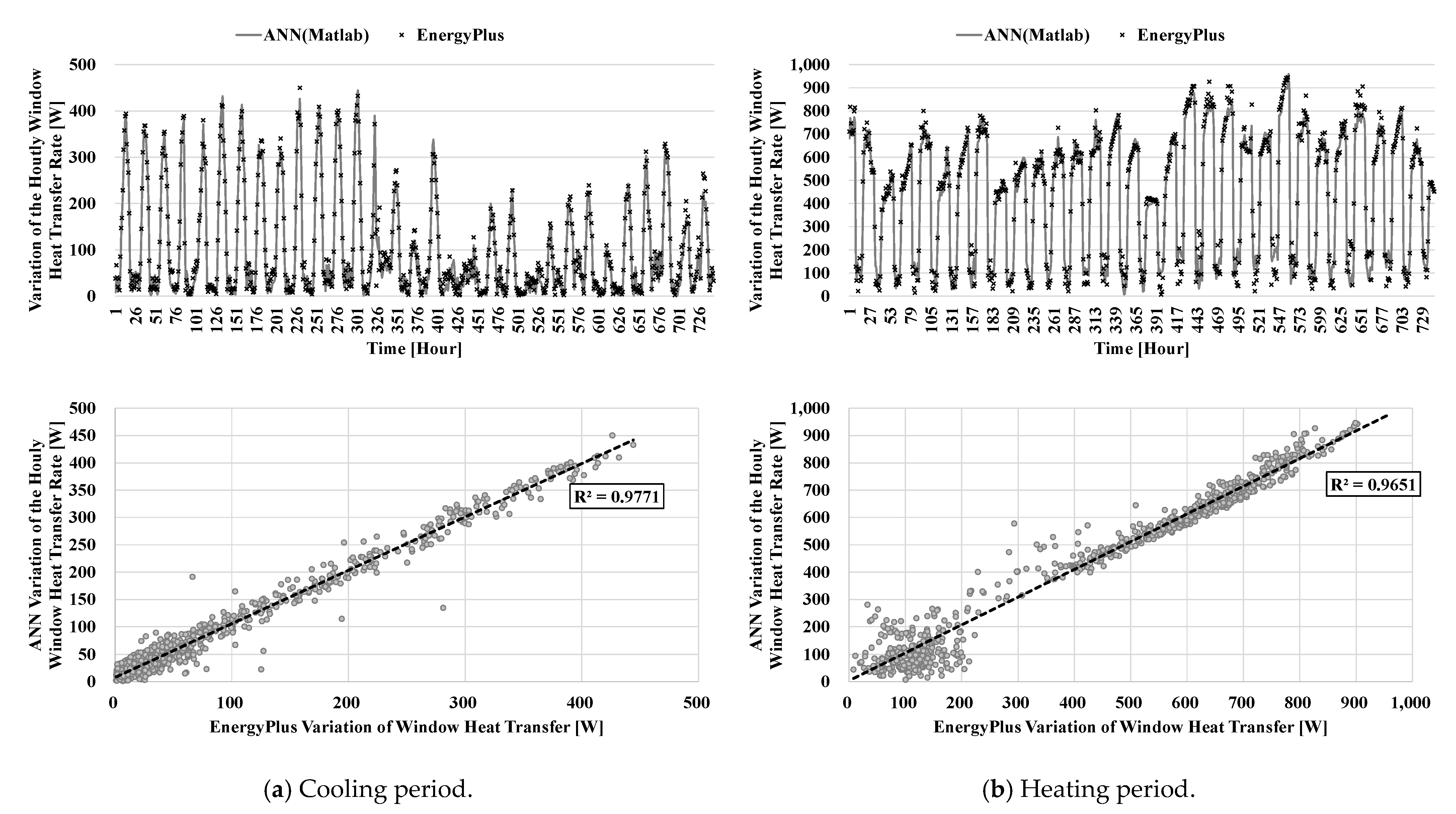
To evaluate the accuracy of the ANN-based optimal control model during the integrated simulation, the simulation results of the ANN (MATLAB) and EnergyPlus were compared. Figure 8 shows the performance evaluation results of the integrated simulation.

According to the performance evaluation of the integrated simulation, the window heat transfer predicted by the ANN and EnergyPlus was similar in the cooling and heating periods. The R² value for the cooling period was 0.977, and that for the heating period was 0.965. Therefore, the optimal control model based on ANN is expected to be highly accurate during integrated simulation operations.

6.2. Analysis of Window Heat Transfer

The goal of this research was optimal control of the movable shading device to minimize the changes in window heat transfer. To this end, this study conducted the integrated simulation and analyzed the window heat transfer. The conduction, convection, and radiation of the window heat transfer were analyzed, and the results without control (slat angle: 45°) and after optimal control using the ANN were compared. Positive (+) values represent heat gain, and negative (−) values represent heat loss.

6.2.1. Cooling Period

This section shows the window heat transfer in the daytime and nighttime in the cooling period with and without optimal control. The indoor temperature, outdoor temperature, inside face temperature, and outside face temperature are considered when the ANN-based optimal control is applied. The inside face temperature and outside face temperature were the internal and external surface temperatures of the window, respectively. 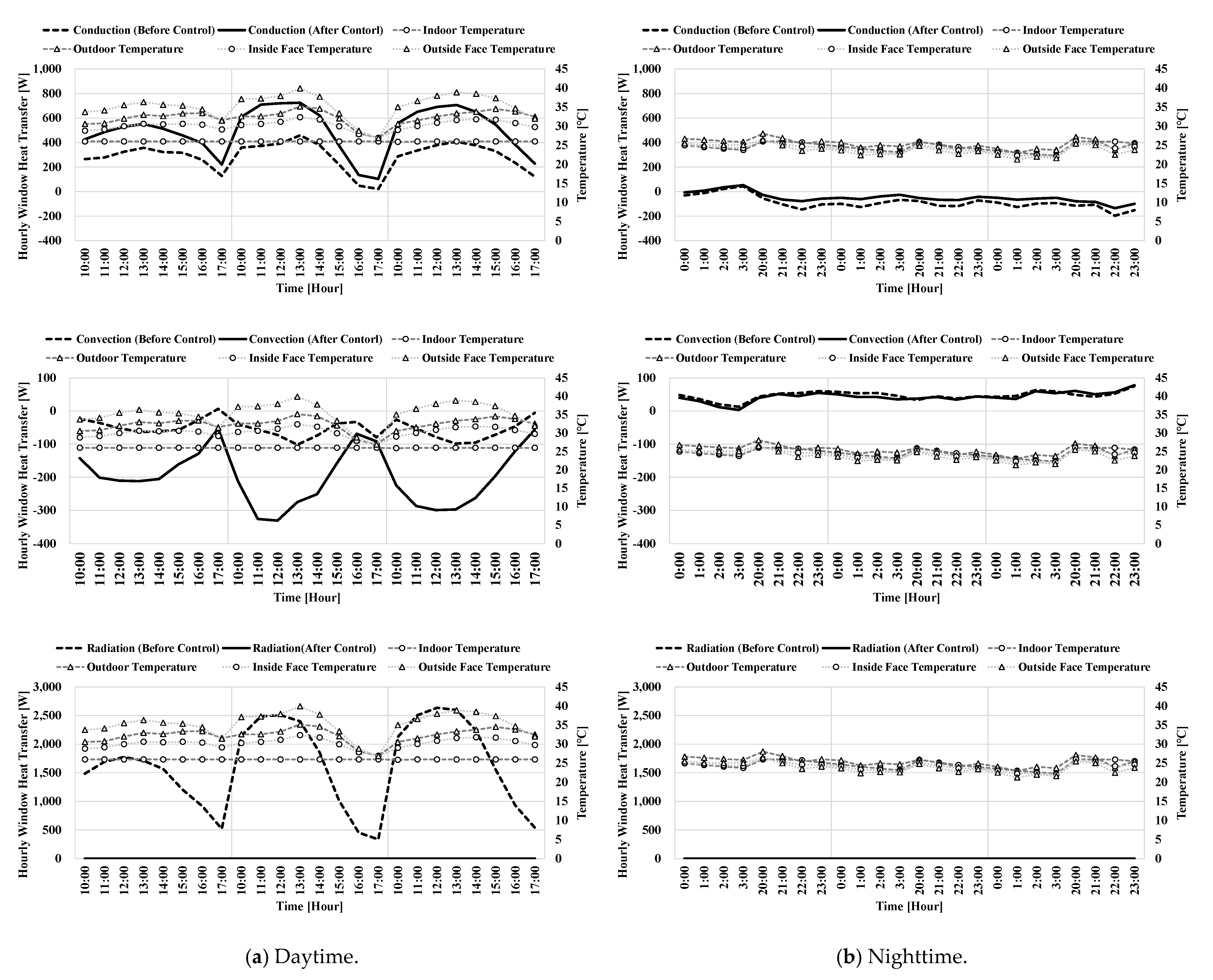Figure 9 presents the hourly window heat transfer in the cooling period.

According to the analysis of the daytime window heat transfer, conduction heat transfer provided a heat gain of approximately 50 to 250 Wh. This result suggests that heat flows from outside to inside because the external surface temperature of the window was higher than its internal surface temperature. Convection heat transfer produced a heat loss of approximately 50 to 350 Wh. The reason was that the external surface temperature of the window was higher than the outdoor temperature, and thus the heat was discharged from inside to outside. By contrast, radiation heat transfer was completely blocked. The results indicated that during the daytime in the cooling period, blocking radiation heat transfer was the key control element for minimizing the change in window heat transfer.

According to the analysis of the nighttime window heat transfer, the differences between conduction and convection heat transfer were minimal; however, as in the daytime pattern, conduction heat transfer resulted in a heat gain, and convection heat transfer resulted in a heat loss. Because there was no solar radiation in the nighttime, no difference in radiation heat transfer was observed.

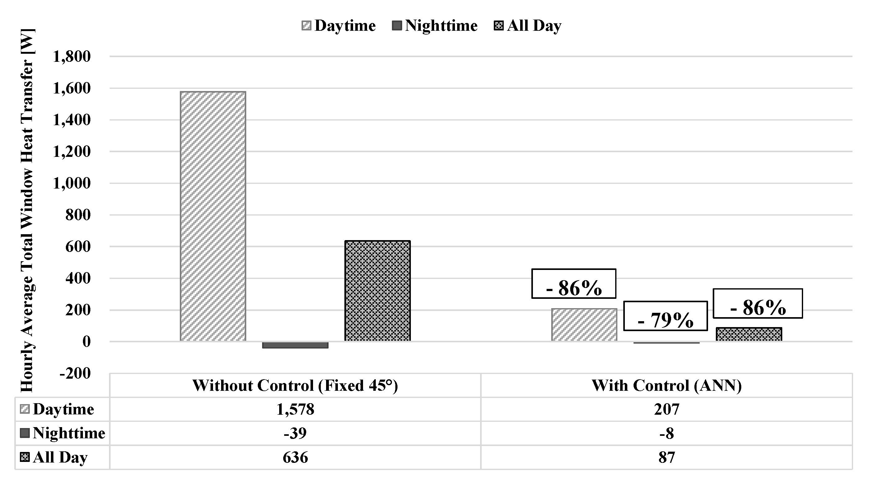
The total window heat transfer with and without optimal control was also analyzed. The hourly average total window heat transfer in the daytime, in the nighttime, and all day were analyzed. Figure 10 presents the hourly average total window heat transfer in the cooling period.

According to the analysis of the hourly average total window heat transfer, the values for the daytime, nighttime, and the entire day decreased by approximately 86%, 79% and 86%, respectively, on average after the optimal control was applied compared to the values without optimal control. The results suggest that if the optimal control model is applied in the cooling period, the total window heat transfer could be expected to decrease.

6.2.2. Heating Period

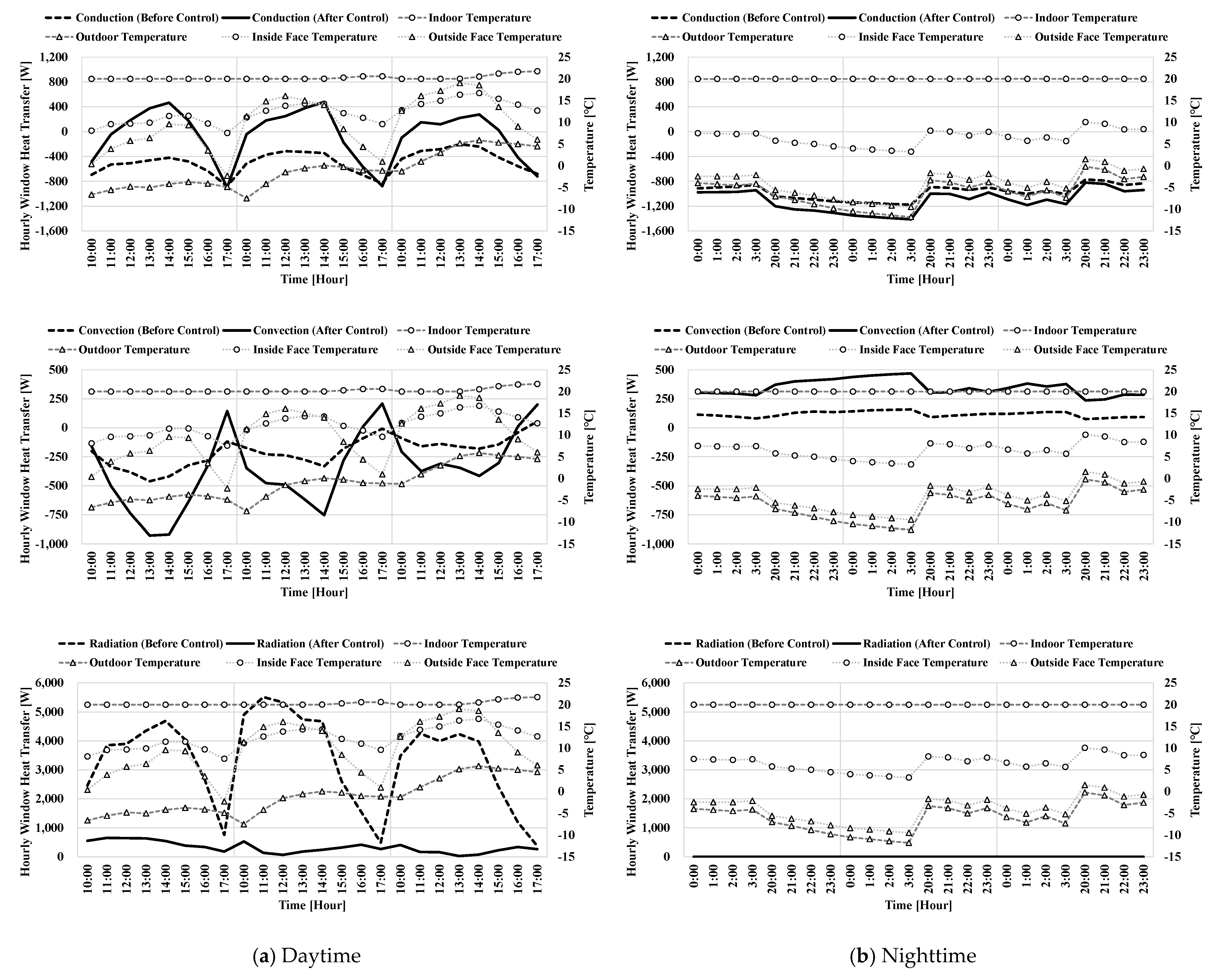
This section presents the window heat transfer results for daytime and nighttime during the heating period. In this section, indoor temperature, outdoor temperature, inside face temperature, and outside face temperature are considered when the ANN-based optimal control is applied, as in Section 6.2.1. Figure 11 shows the hourly window heat transfer results for the heating period.

According to the analysis of the daytime window heat transfer, conduction heat transfer resulted in both heat gain and loss phenomena of approximately 200 to 800 Wh. The reason for this was the changes in the external and internal surface temperatures of the window. Convection heat transfer resulted in a heat loss of approximately 0 to 450 Wh. This result suggests that heat was discharged from inside to outside because the external surface temperature of the window was higher than the outdoor temperature. By contrast, radiation heat transfer decreased from approximately 500 to 4000 Wh. Moreover, unlike the cooling period, in which radiation heat transfer was completely blocked, in this period, radiation heat transfer of approximately 500 Wh was observed. The results indicate that the inflow of solar radiation could help reduce the building heating load during the heating period.

According to the analysis of the nighttime window heat transfer, in contrast to the cooling period, a difference was found between conduction and convection heat transfer. Conduction heat transfer produced a heat loss of approximately 100 to 200 Wh. The reason is heat discharge from inside to outside, which occurs because the window internal surface temperature was higher than the external surface temperature. Convection heat transfer provided a heat gain of approximately 250 Wh, which is different from the predicted result. The reason was that heat loss was expected to occur owing to the difference between the outdoor temperature and window external surface temperature. However, convection heat transfer was significantly affected by the wind speed. Therefore, the wind speed may be higher during nighttime in the heating period. By contrast, there was no solar radiation in the nighttime, and thus the radiation heat transfer did not change.

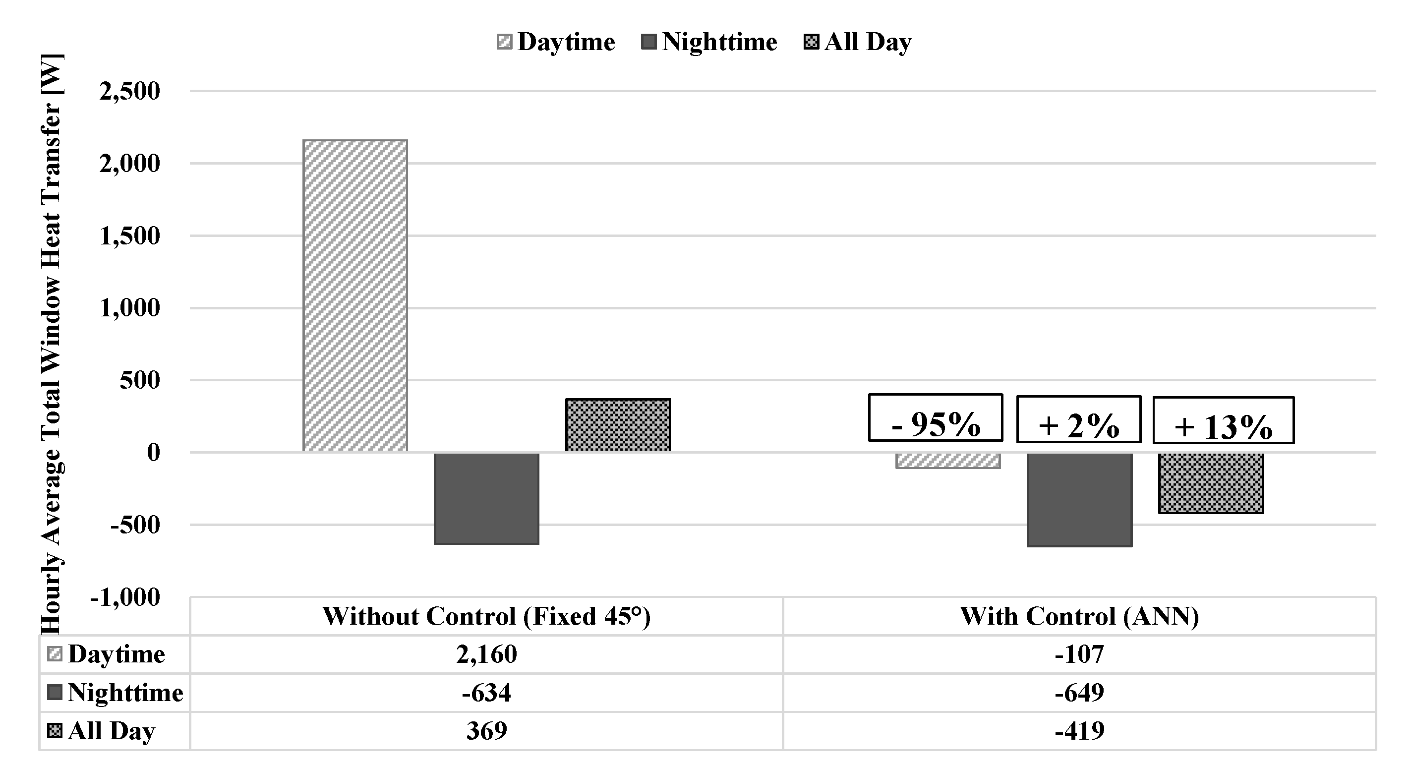
The total window heat transfer with and without optimal control was also analyzed, as in Section 6.2.1. Figure 12 presents the hourly average total window heat transfer results for the heating period.

The hourly average total window heat transfer was decreased by 95% on average in the daytime, whereas it increased by 2% on average in the nighttime when optimal control was applied compared to the values obtained without optimal control. Moreover, the heat transfer for the entire day increased by 13% on average. This result suggests that the effects of conduction and convection on the hourly average total window heat transfer increase in the nighttime and thus affect the total window heat transfer.

6.2.3. Total Window Heat Transfer and Slat Angle

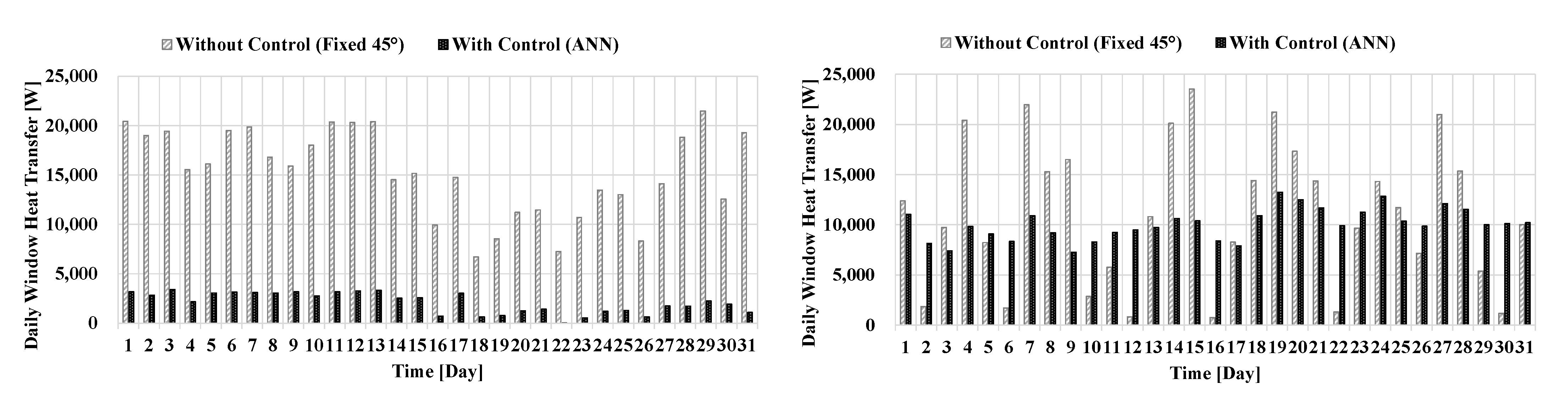
In this section, the total window heat transfer with and without optimal control and the effect of slat angle under optimal control were analyzed. Hourly, peak and monthly analyses of the total window heat transfer were conducted, and the decrease in heat transfer under optimal control was characterized. Increases and decreases in heat transfer were not considered in terms of losses and gains, and only the total window heat transfer was considered. Figure 13 shows the window heat transfer with and without optimal control.

The daily total window heat transfer without optimal control was approximately 15,000 W/day on average during the cooling period. By contrast, it was approximately 11,500 W/day on average during the heating period. Therefore, optimal control was applied to reduce the total window heat transfer. The daily total window heat transfer with optimal control decreased to approximately 2000 W/day on average during the cooling period and to approximately 10,000 W/day on average during the heating period. The optimal control model was expected to decrease window heat transfer by 86% and 13% during the cooling and heating periods, respectively.

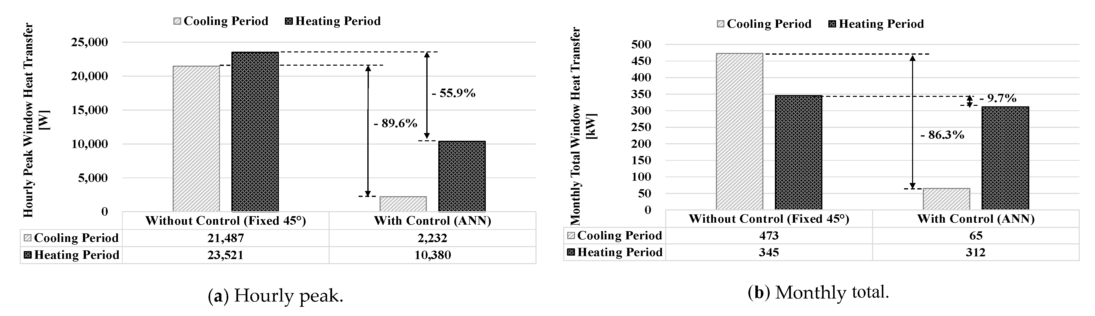
The window peak load and monthly window load were analyzed to identify changes in the load through the window. Figure 14 shows these changes with and without optimal control.

When optimal control was applied, the window peak load decreased by 89.6% and 55.9% during the cooling and heating periods, respectively. Furthermore, the monthly window heat transfer decreased by 86.3% and 9.7% during the cooling and heating periods, respectively. Therefore, if the optimal control model is applied, the building energy load through the window is expected to be reduced, and an active response to the load change is possible.

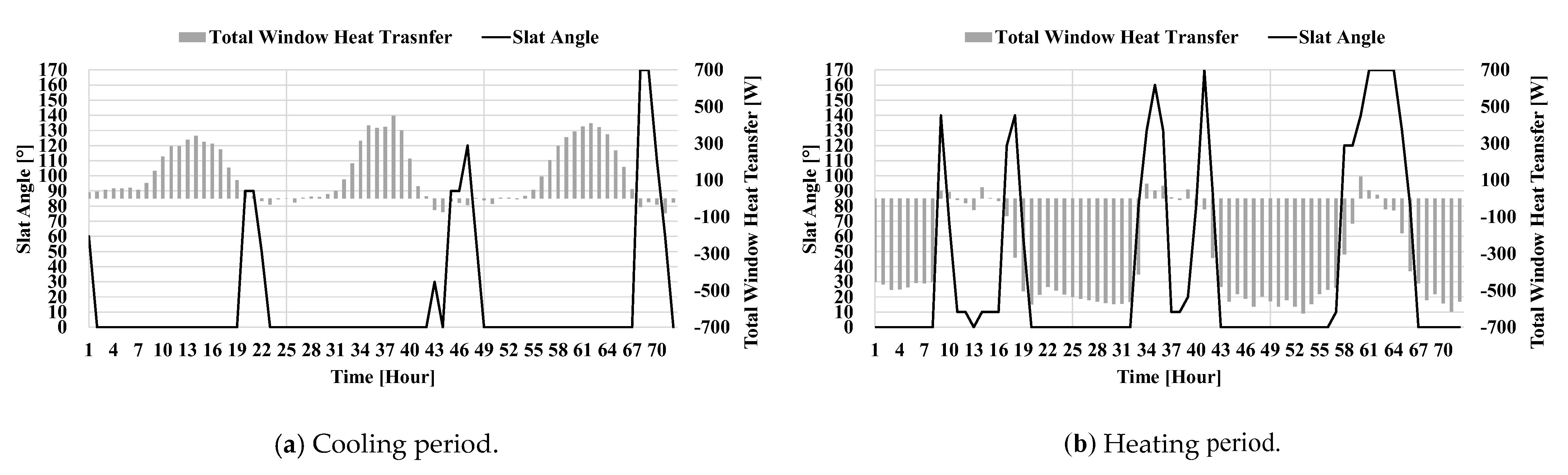
In this study, the slat angle response of the optimal control model was analyzed according to the analysis shown above. Figure 15 presents the changes in slat angle under optimal control.

During the cooling period, the slat angle of the movable shading device was 0° in the daytime and between 90° and 170° in the nighttime. By contrast, during the heating period, it was 120°–170° in the daytime and 0° in the nighttime. The slat angle settings during the cooling and heating periods showed opposite results. During the cooling period, heat gain was blocked in the daytime, and heat transfer occurred in the nighttime. These results would help reduce the building cooling load by heat emission. During the heating period, either heat flowed in, or heat loss was minimized in the daytime, and heat loss was minimized in the nighttime. These results would help reduce the building heating load by retaining heat. These results show that solar radiation was not an absolute factor in determining the slat angle. It was observed that the slat angle was determined based on combined heat transfer amount, including conduction, convection, and radiation.

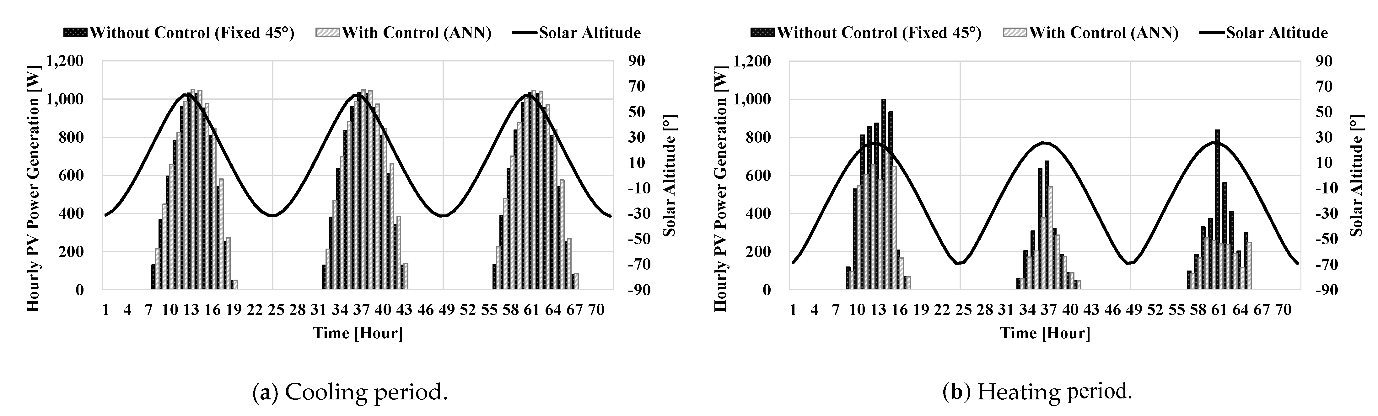
6.3. PV Power Generation

In this section, this study evaluated the PV power generation with and without ANN optimal control of the movable shading device. An energy network was materialized that can remove the load generated by window heat transfer using PV power generation. For this purpose, the PV power generation with and without optimal control was analyzed. Figure 16 shows the hourly PV power generation at various solar altitudes. The reason this study compared the PV power generation at different solar altitudes was that the solar altitude exhibits seasonal variation. In addition, the changes in solar altitude affect the solar radiation that enters at each slat angle and consequentially affects the PV power generation.

According to the analysis, when optimal control was applied, the hourly PV power generation increased approximately 10.8% against the case without control in the cooling period. On the other hand, it decreased about 28.8% in the heating period. Accordingly, during the cooling period, the optimal control model could simultaneously reduce window heat transfer and increase PV power generation. During the heating period, the optimal control model could reduce window heat transfer but could not increase PV power generation. In the future, during the heating period, additional control methods to minimize the loss of the PV power generation is required. Furthermore, the PV power generation was higher during the cooling period than during the heating period. The reasons for this phenomenon appeared to be lower solar altitude in the heating period and less projected slat surface area to intake solar radiation.

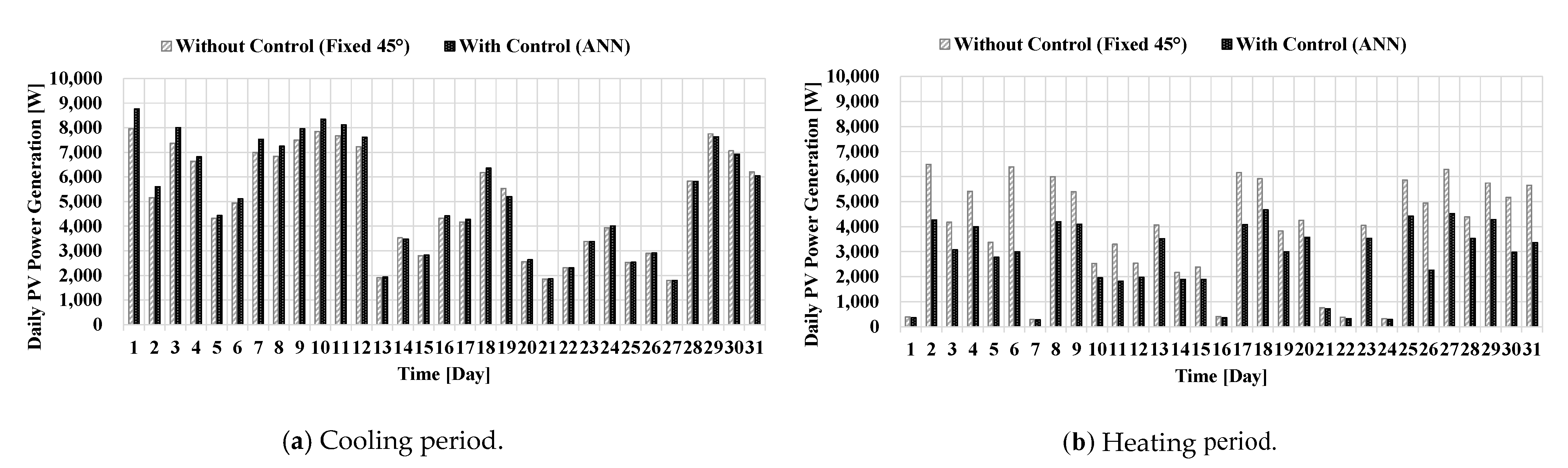
Figure 17 presents the daily PV power generation with and without optimal control of the shading device to minimize window heat transfer.

In the cooling period, the daily PV power generation was up to 8000 W/day without optimal control and up to 8800 W/day with optimal control. On the other hand, in the heating period, the daily PV power generation was up to 6500 W/day without optimal control and up to 4700 W/day with optimal control.

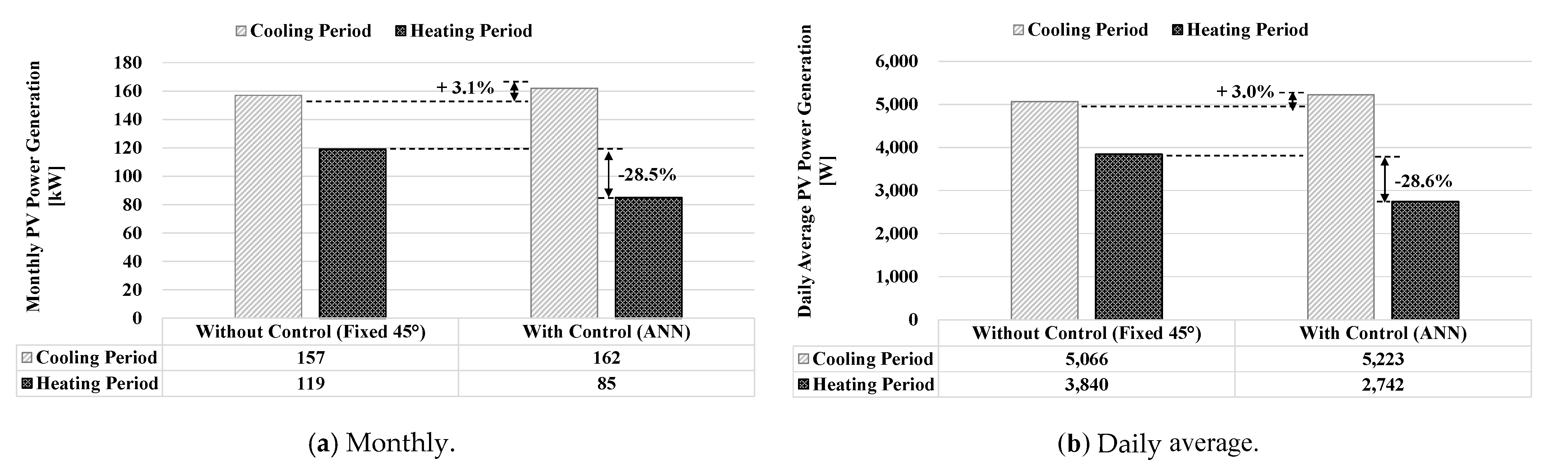
Figure 18 shows the PV power generation with and without optimal control.

The daily average and monthly PV power generation under optimal control increased by 3.0% and 3.1% during the cooling periods and decreased by 28.5% and 28.6% during the heating period. Therefore, in the cooling period, the optimal control model reduces the window heat transfer and results in larger PV power generation; thus, it would be favorable in terms of PV power generation in the cooling period.

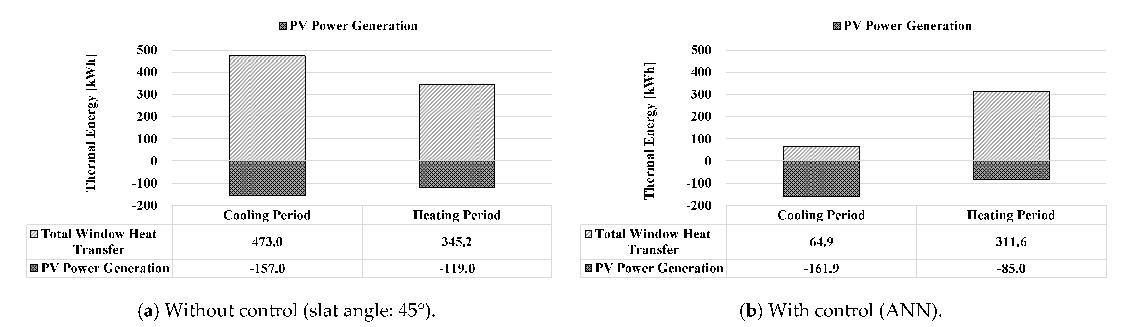
This study materialized the energy network that can remove window thermal energy using PV power generation on the basis of the above analysis results. Figure 19 shows the results of an analysis of the window thermal energy network with and without optimal control. In this figure, PV power generation is indicated by negative (−) numbers to indicate decreased window heat transfer.

The PV power generated without optimal control reduced the window heat transfer by 33.2% and 34.5% in the cooling and heating periods, respectively. By contrast, the PV power generated under optimal control reduced the window heat transfer by 100% and 27.3% during the cooling and heating periods, respectively. Furthermore, in the cooling period, PV power generation produced approximately 97 kWh of additional electric power while reducing window heat transfer. Therefore, the optimal control model is expected to control changes in the building load effectively and actively.

7. Summary and Conclusions

Among various factors affecting fluctuations in building energy use, the window was the most significant. The reason was that windows are the most thermally vulnerable building structures. Therefore, it is essential to reduce energy changes at windows.

This study considered that decreasing window heat transfer would reduce the effects on the building load. To achieve this goal, a shading device was used. Moreover, the energy was produced by attaching a PV device to the shading device, and this energy offsets the energy produced by window heat transfer, which contributes to fluctuations in the building load. The proposed system was applied by developing an optimal control model for active control in response to changes in the external environment, in contrast to existing methods. Optimal control models were developed for the cooling and heating periods. These models used an ANN. To clarify and readability the conclusions, this study summarized them in three parts (accuracy of the ANN model, window heat transfer, and PV power generation). The following conclusions were obtained.

• The ANN-based optimal control model was composed of 15 hidden neurons and 1 hidden layer. The cvRMSE of this model was 9.9% and 9.8% for the cooling and heating periods, respectively. Moreover, R² was greater than 0.99 in all cases. These results suggest that the optimal control model is highly accurate. In an integrated simulation using the ANN-based optimal control model, R² values of the cooling period and heating period control models were 0.977 and 0.965, respectively. Therefore, the developed ANN-based optimal control model was expected to show high accuracy during an integrated simulation.
• Most window heat transfer occurred by radiation heat transfer, followed by conduction and convection heat transfer, in that order, in both the cooling and heating periods. The daytime window heat transfer change was found to be more significant than the nighttime change. Moreover, the ANN-based optimal control model established different heat gain and discharge plans for each component (conduction, convection, and radiation transfer). Finally, reducing the effects of radiation was found to be the key factor in minimizing the window heat transfer. According to an analysis of the total window heat transfer with/without optimal control, the window peak load decreased by 89.6% and 55.9% during the cooling and heating periods, respectively. Furthermore, the monthly window load decreased by 86.3% and 9.7% in the cooling and heating periods, respectively. Therefore, the optimal control model can decrease the building energy through windows.
• An analysis of the slat angle showed that heat gain was blocked in the daytime and heat entered during the nighttime in the cooling period. During the heating period, both the daytime and nighttime heat loss were minimized. Therefore, the optimal control model could help reduce the cooling load in the cooling period and the heating load in the heating period. Based on the analysis associated with the PV power generation with/without optimal control, the power generation increased by 3.0% in the cooling periods under optimal control. Furthermore, an average of 157 W per day and 5 kW per month of additional power were obtained during the cooling period. However, the power generation decreased by 28.5% in the heating periods. In addition, an average of 1 kW per day and 34 kW per month were obtained during the heating period. It could be concluded that, therefore, the optimal control model generated more PV power only during the cooling period.

This study’s results are useful for analyses of window heat transfer and additional power generation of the PV. The optimal control model developed in this study has excellent potential for managing building load changes effectively and actively. However, this model was developed considering only the cooling and heating periods, and it may perform differently in various other periods (e.g., inter-seasonal periods). Therefore, it is necessary to consider additional periods in future work. If optimal control during various periods was considered, this method would become more reliable. In this study, however, the PV power generation decreased during the heating period. Therefore, as one of the future studies, a new control method would be developed to minimize the PV power generation’s loss by the slat angle control.

References

- Lee, C. Results of the 21st Paris Climate Change Conference. In Proceedings of the Report of the Conference of the Parties on Its Twenty-first Session, Paris, France, 30 November–13 December 2015; Korea Research Institute on Climate Change: Seoul, Korea, 2015. [Google Scholar]
- Office for Government Policy Coordination. Frame Act on Low Carbon and Green Growth. Act No. 16133, 31 December 2018. Available online: https://elaw.klri.re.kr/kor_service/lawView.do?hseq=49999&lang=ENG (accessed on 10 December 2020).
- National Greenhouse Gas Inventory Report of Korea; Greenhouse Gas Inventory and Research Center (GIR): Seoul, Korea, 2017.
- Jeong, S.Y.; Baek, N.C.; Yoon, J.H.; Shin, U.C.; Kim, Y.K.; Kang, S.H. The Study on Energy Performance Measurement and Energy Self-sufficiency Analysis of KIER Zero Energy Solar House II. J. Archit. Inst. Korea Plan. Des. 2011, 27, 307–314. [Google Scholar]
- Ministry of Land, Green Buildings Construction Support Act. Act No. 15728, 14 August 2018. Available online: https://elaw.klri.re.kr/kor_service/lawView.do?hseq=50008&lang=ENG (accessed on 10 December 2020).
- Jung, D.E.; Lee, C.; Do, S.L. Analysis of the Window Glazing Heat Transfer of Installation of an External Shading Device. Korean J. Air Cond. Refrig. Eng. 2020, 32, 278–287. [Google Scholar]
- Palmero-Marrero, A.I.; Oliveira, A.C. Effect of Louver Shading Devices on Building Energy Requirements. Appl. Energy 2010, 87, 2040–2049. [Google Scholar] [CrossRef]
- Bellia, L.; Falco, F.D.; Minichiello, F. Effects of Solar Shading Devices on Energy Requirements of Standalone Office Buildings for Italian Climates. Appl. Therm. Eng. 2013, 54, 190–201. [Google Scholar] [CrossRef]
- Mandalaki, M.; Papantoniou, S.; Tsoutsos, T. Assessment of Energy Production from Photovoltaic Modules Integrated in Typical Shading Devices. Sustain. Cities Soc. 2014, 10, 222–231. [Google Scholar] [CrossRef]
- Kim, S.H.; Kim, I.T.; Choi, A.S.; Sung, M.K. Evaluation of Optimized PV Power Generation and Electrical Lighting Energy Savings from the PV Blind-integrated Daylight Responsive Dimming System Using LED Lighting. Sol. Energy 2014, 107, 746–757. [Google Scholar] [CrossRef]
- Hong, X.; He, W.; Hu, Z.; Wang, C.; Ji, J. Three-dimensional Simulation on the Thermal Performance of a Novel Trombe Wall with Venetian Blind Structure. Energy Build. 2015, 89, 32–38. [Google Scholar] [CrossRef]
- Zhang, W.; Lu, L.; Peng, J. Evaluation of Potential Benefits of Solar Photovoltaic Shadings in Hong Kong. Energy 2017, 137, 1152–1158. [Google Scholar] [CrossRef]
- Hong, S.; Kim, I.T.; Choi, A.S. Analysis of Indoor Luminous Environment and Power Generation by Roll Screen and Venetian Blind with PV Modules. Eur. J. Sustain. Dev. 2017, 6, 302–308. [Google Scholar]
- Hong, S.; Choi, A.S.; Sung, M. Impact of Bi-directional PV Blind Control Method on Lighting, Heating and Cooling Energy Consumption in Mock-up Rooms. Energy Build. 2018, 176, 1–16. [Google Scholar] [CrossRef]
- International Energy Conservation Code; International Code Council (ICC) Inc. IECC: Falls Church, VA, USA, 2009.
- EnergyPlus Ver. 8.5. Available online: https://energyplus.net/ (accessed on 10 December 2020).
- MathWorks Ver. 2016. Available online: https://www.mathworks.com/ (accessed on 10 December 2020).
- Building Controls Virtual Test Bed Ver. 1.6.0. Available online: https://simulationresearch.lbl.gov/bcvtb/FrontPage (accessed on 10 December 2020).
- Marquardt, D.W. An Algorithm for Least-squares Estimation of Nonlinear Parameters. J. Soc. Ind. Appl. Math. 1963, 11, 431–441. [Google Scholar] [CrossRef]
- International Weather for Energy Calculations 2.0; American Society of Heating, Refrigerating and Air-Conditioning Engineers (ASHRAE): Peachtree Corners, GA, USA, 2017.
- Yang, I.H.; Yeo, M.S.; Kim, K.W. Application of Artificial Neural Network to Predict the Optimal Start Time for Heating System in Building. Energy Convers. Manag. 2003, 44, 2791–2809. [Google Scholar] [CrossRef]
- Moon, J.W.; Kim, K.; Min, H. ANN-based Prediction and Optimization of Cooling System in Hotel Rooms. Energies 2015, 8, 10775–10795. [Google Scholar] [CrossRef]
Figure 1.
Diagram of the overall research process.
Figure 2.
3D view of a building model.
Figure 3.
Diagram of movable shading device integrated with the photovoltaic (PV) at various slat angles.
Figure 4.
Conceptual diagram of integrated simulation.
Figure 5.
Mean squared error (MSE) analysis of neural network (ANN) optimal control model.
Figure 6.
Regression analysis of ANN optimal control model.
Figure 7.
Diagram of the window heat transfer and PV power generation.
Figure 8.
Comparison of window heat transfer in integrated simulation.
Figure 9.
Hourly window heat transfer during the cooling period.
Figure 10.
Hourly average total window heat transfer during the cooling period.
Figure 11.
Hourly window heat transfer during the heating period.
Figure 12.
Hourly average total window heat transfer during the heating period.
Figure 13.
Total window heat transfer with and without ANN optimal control.
Figure 14.
Reduction in window heat transfer with and without ANN optimal control.
Figure 15.
Variation in slat angle under ANN optimal control.
Figure 16.
PV power generation with and without ANN optimal control.
Figure 17.
Figure 18.
Variation in PV power generation.
Figure 19.
Thermal energy network between window heat transfer and PV power generation.