1. Introduction
In response to increasing competition and regulatory pressure, the food processing and chemical industries are seeking some solutions to limit energy demands. One of the ways is to increase overall processes efficiency and limit the environmental impact of their production. Moreover, competitive conditions force the use of computer simulations at every stage of product design. Process modeling directly influences the effectiveness of the process as well as its expenses [
1,
2,
3]. The scale of products manufactured in large quantities and with low margins significantly increases the importance of effective design and process optimization [
4]. The process design and modelling influence the industrial engineering practice. Moreover, it leads to the continuous improvement of the practical skills of engineers [
5,
6].
During the various stages of process and equipment design, computational packages, known as process simulators, are used to model flowsheet configurations [
7,
8]. Such flowsheet configurations are often highly integrated, to improve efficiency and profitability [
9,
10]. Modeling often refers to the determination of material and energy balances for a designed product, along with the necessary constitutive relations. The simulation includes (numerical) approaches to solving the previously mentioned balance equations [
11]. Optimizations can be used to improve products at various stages. At the conceptual level, the optimal flowchart is selected from a set of possible solutions (usually based on abbreviations/approximate representations of unit operations). On the other hand, the detailed design consists of determining the dimensions of the device and its operating conditions (pressure, temperature, flow rate). The use of computer techniques allowed for the building of a detailed process structure [
12,
13,
14].
In the 1950s, the food and chemical industries’ development of simulation tools for individual unit operations began [
15]. The advantages of that improvement included the decrease in economical spending [
16,
17,
18,
19]. The use of computer techniques has become a daily practice in companies that are able to invest in the purchase and implementation of commercial simulation software. Teams of researchers dealing with process systems engineering have made a significant contribution to the development of large-scale process optimization [
20,
21]. Actually, some of the existing commercial process simulation packages offer very extensive optimization solutions. Computational optimization is often carried out with simplified process models or by considering only parts of the flowsheet [
5]. Despite many solutions existing in the field of optimization, there are many examples that explain the reasons for the discrepancy between research progress, software capabilities, and the implementation of specific solutions in practice [
17,
20]:
No clear conviction whether the application of rigorous optimization techniques is correct, e.g., due to uncertainties related to the system parameters (physical properties).
No evidence that hardware costs can be reduced when practically using optimization results, especially in the early stages of conceptual design.
Problems with the proper definition of the tasks, including the determination of decision variables and existing constraints.
Difficulties in estimating the necessary preparation time and calculations in situations with tight timeframes for project implementation. This is often directly related to the robustness of numerical algorithms and their reliability (highly nonlinear systems, complex systems of equations), for which it is difficult to accept possible preliminary assumptions [
22,
23,
24,
25].
2. Background and Description of the Study Approach
Reliable operation is critical if food processing plants are to meet their production targets. For just-in-time plants, stopping production can result in lost sales and unmet demand, which has a direct impact on profit. These downtimes can affect selected operations in the plant, subsystem operations or single unit operations. One of the factors that may disrupt the production process in a plant and the functioning of its installations is the formation of foam in the pumped liquids.
Foam is a dispersed gaseous phase in a small amount of liquid. The presence of surface-active substances (surfactants) facilitates the formation of foam, by reducing surface tension and increasing viscosity. The foam forming requires an appropriate volume fraction of gas relative to the solution of surfactants for each system, e.g., the dispersed systems (suspensions, emulsions). In this case, the foam is characterized by high complexity, as described in detail by Tsay et al. [
25]. As an effect of intensive mechanical, chemical, and thermal processes, foam adversely affects the course of technological processes by randomly changing the physicochemical properties of the pumped liquid. The most important negative impacts related to the formation of foam in liquids include:
Disturbances to the proper operation of conventional pumps, resulting from the variability of liquid inflow (reduction in mass flow) to the rotors.
Mass fluctuation of the liquid flowing into equipment on the process line, causing difficulties in maintaining the required process parameters.
Unstable flow in pipelines leading to measurement errors for flow rate, liquid density, and pressure, resulting in incorrect input data for automatic process control.
Such problems require steps to limit or eliminate the formation of foam. Physical and chemical methods of foam destruction are commonly applied. Chemical methods include the use of anti-foaming agents, which may also act as inhibitors, depending on the stage of the process. Physical methods of foam breaking include mechanical transmission of stress via contact with the blade of the breaking element. Another physical method of foam destruction is ultrasound, which has been discussed extensively [
26,
27,
28,
29,
30].
Chemical methods of defoaming, although widespread, have drawbacks. Most importantly, they may affect the course of reactions in the liquid and cause contamination, which is in some cases unacceptable [
29]. The chemicals used must meet a number of requirements like safety [
30]. Many anti-foaming agents are added to products intended for human consumption. Sometimes substances used to regulate the formation of foam must be removed during the treatment process, as in the production of baking yeast [
31]. The chemical elimination of foam has been discussed by P.R. Garret [
32,
33] as well as Exerowa et al. [
34].
Although manufacturers state that chemical anti-foaming agents pose no risk to health and preserve all the valuable sensory and nutritional properties of food, there is an increasing preference for physical methods of foam elimination. This is especially true among small food producers, who can then present their products as healthy and natural. However, physical methods also have several drawbacks. Frequently, large devices are used with relatively low performance parameters and high energy usage. Moreover, the foam produced during production processes is removed, but the tendency of the liquids to form foam is not eliminated.
In this study, computer simulations and bench tests of a pump with a special design were conducted that allows for the transport of dispersive foaming liquids and simultaneous separation of the liquid and gaseous phases. The liquid phase can be used in further technological processes, whereas the gaseous phase is removed from the hydraulic system. Due to the lack of mathematical models for performing pump calculations, it was decided to use process modelling techniques based on CFD (Computer Fluid Dynamics) tools. The results of simulations were compared with the bench tests on the pump prototype, enabling validation of the numerical model.
3. Materials and Methods
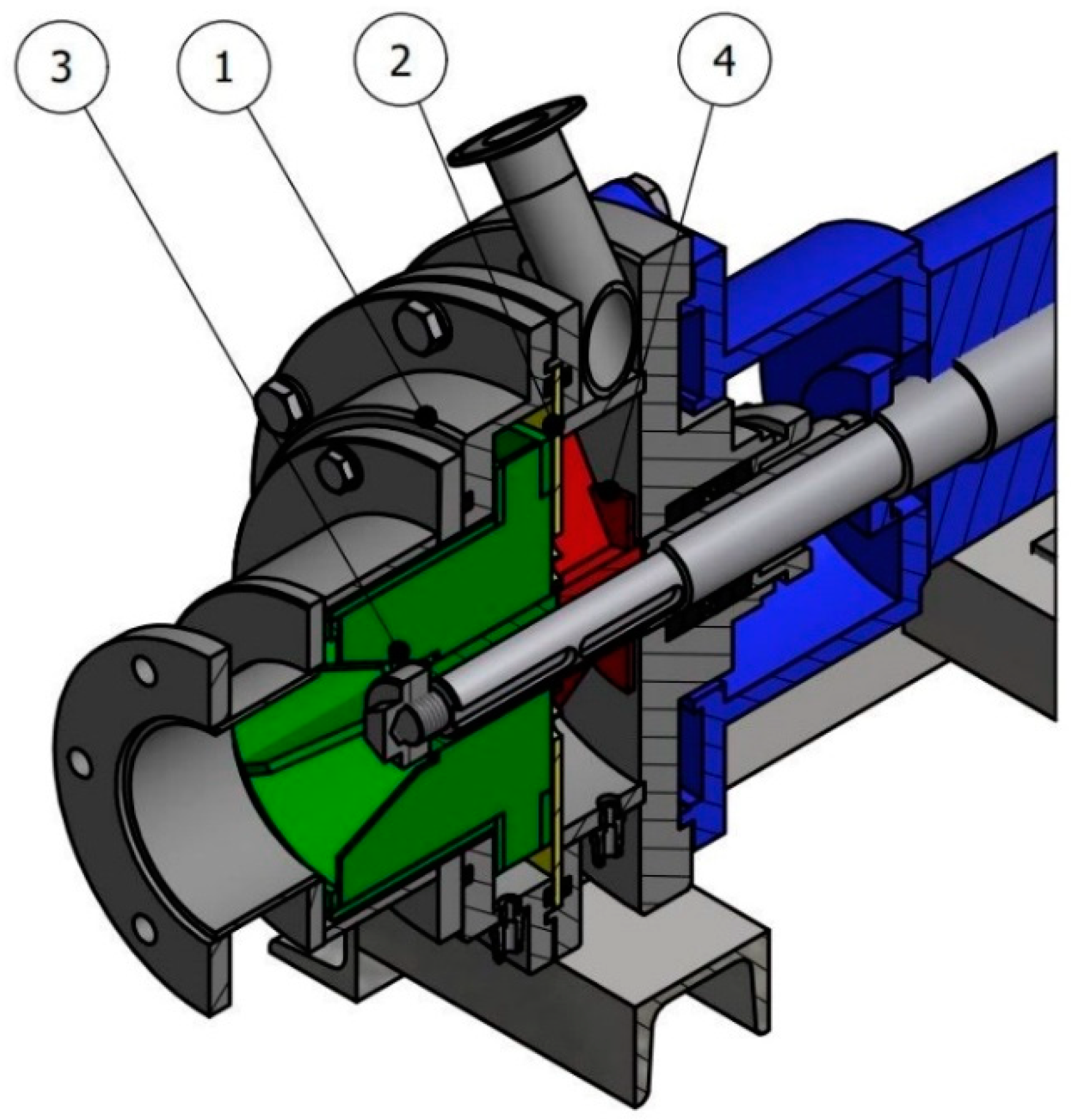
Figure 1 shows a diagram of the skimming pump. It consists of a chamber (1) divided by a partition with holes (2) and two rotors mounted on a common shaft. The first rotor separates the foam and pumps the liquid (3). The second rotor (4), in a two- or three-stage destruction process, mechanically breaks up the foam and removes air and liquid residues. The pump consists of two sections placed in a single casing. These sections are separated by a disc perforated with holes. Each of the sections has a rotor. The rotors are attached to a common shaft. The first rotor separates the phases and pumps the liquid. The second rotor mechanically breaks up the foam and removes the air and liquid residues. The applied solution enables the pumping of liquids with high gaseous phase content. In conventional centrifugal pumps, the gaseous phase content must not exceed 4% [
27]. Otherwise, gas accumulates near the axis of the impeller and liquid flow ceases. In the proposed solution, it is possible to pump both uniform and unstable liquids with a gaseous phase content of up to several tens of per cent.
Figure 2 shows a 3D (axionometric) visualization of the designed pump. The rotating impeller (3) introduces a mixture of liquid and foam into the rotation. The hydrodynamic pressure on the outlet pipe creates a liquid ring in the impeller (3). Foam bubbles accumulate near the rotor axis and are partially broken up by the rotating impeller. The foam-free liquid escapes through the outlet pipe to the plant. The gas released and the remaining foam pass through the opening in the baffle (2) and enter the second chamber. The second rotor (4) breaks up the remaining foam and the gas is removed through the second pump outlet. The remaining liquid from the broken foam is also removed through this outlet.
The prototype used for bench tests was characterized by the following parameters:
The assumed parameters refer to a two-phase liquid/gas medium. The nominal pump speed was n = 1400 min−1. The potential users of the pump include primarily small producers of natural foods, including drinks, fruit and vegetable juices, and ecological dairy products.
3.1. Research Stand
A test stand was designed and constructed to verify the results of the numerical analyses.
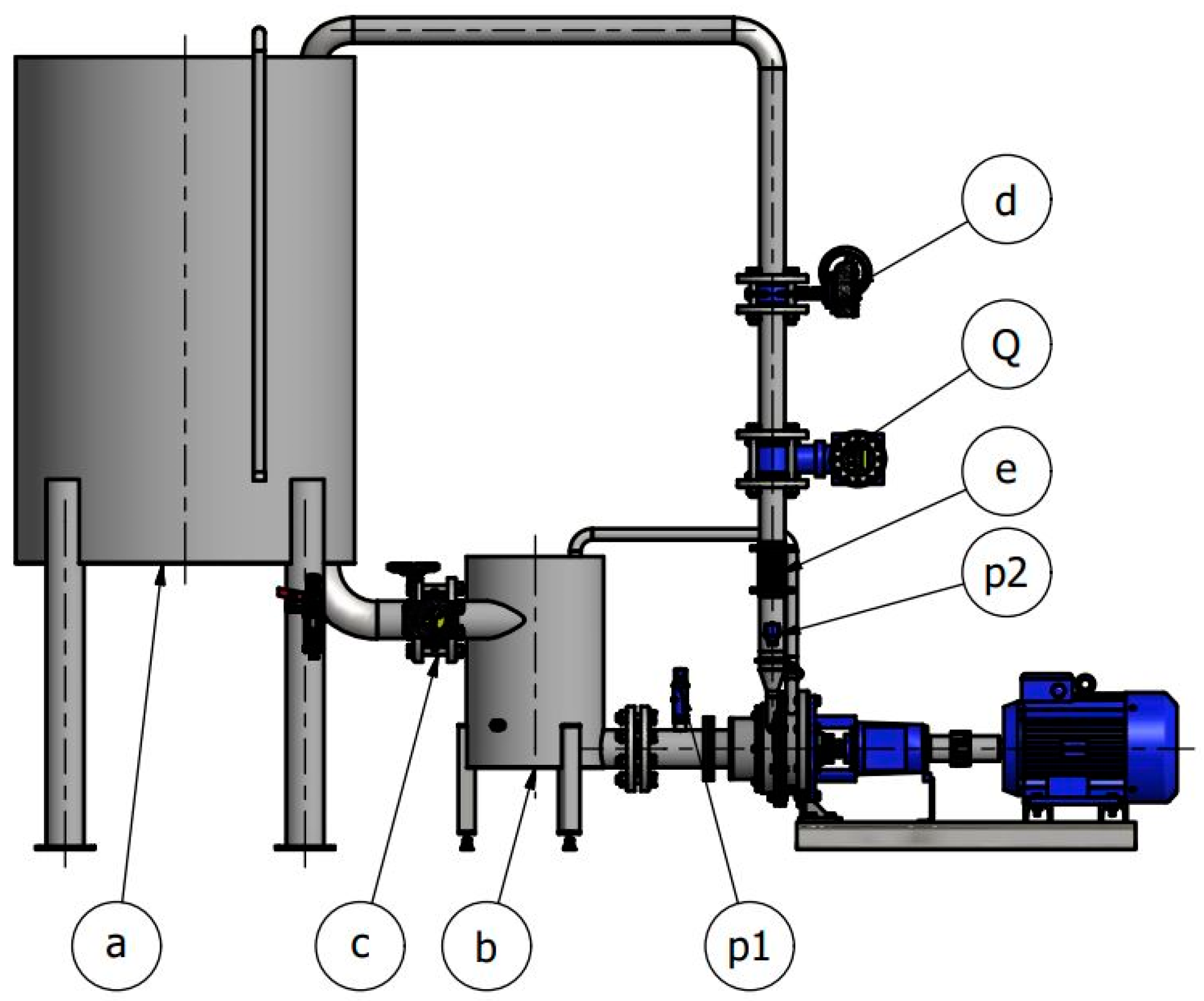
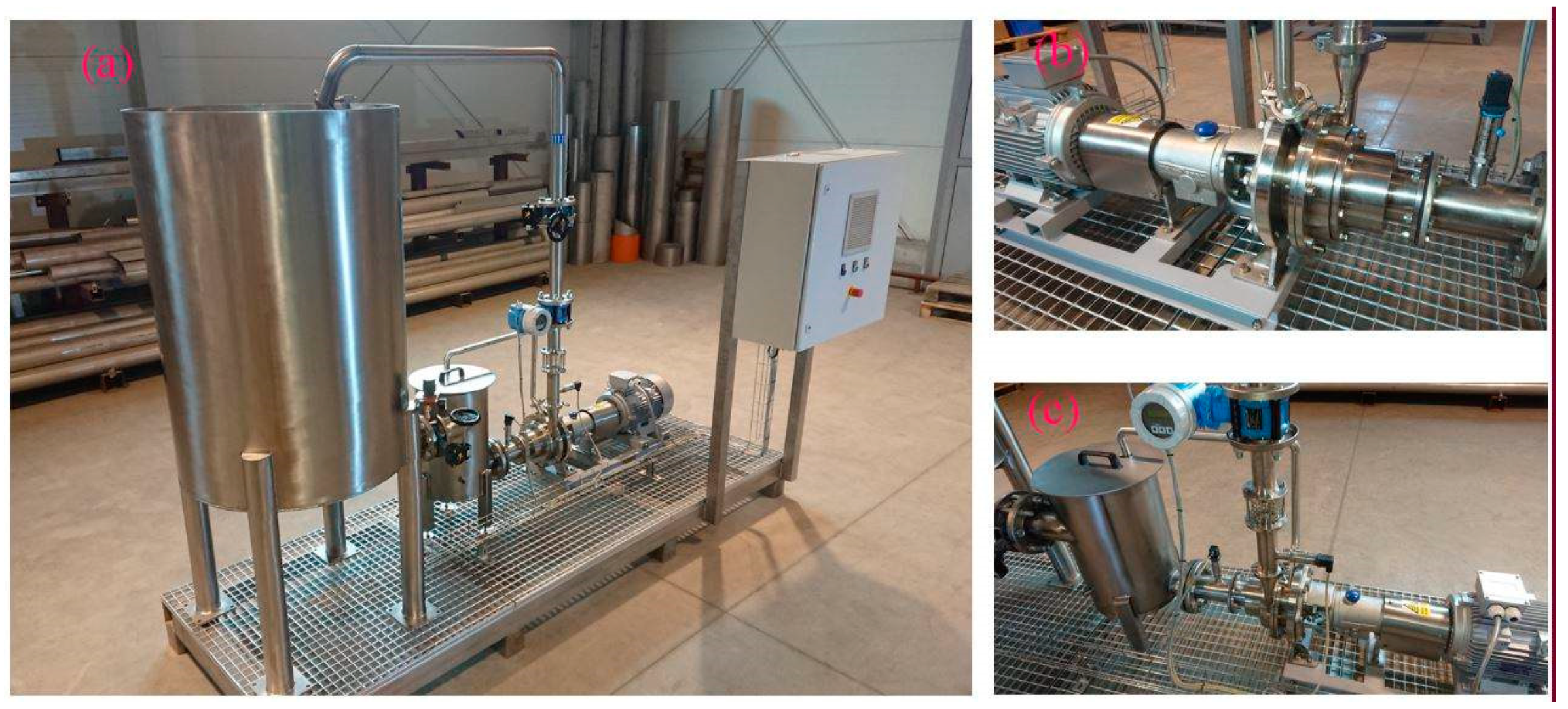
Figure 3 shows a schematic diagram of the test stand, and
Figure 4 shows photos of the test stand. The test stand consisted of a main tank for the pumped liquid (a) and an intermediate tank (b) with a nominal pipeline diameter (d
n) equals 50 mm (c) control damper installed between the tanks. The discharge side of a pump had a 50 mm pipeline, which returns the liquid to the main tank. It also has a 50 mm control throttle (d) and sight glass (e). A d
n = 25 mm pipeline discharges air and residual liquid into the intermediate tank.
Endress Hauser pressure gauges were used for bench measurements. A pressure sensor (p1) type PMP21 with a measuring range of 1–10 bar was mounted at the pump inlet. A pressure sensor (p2) type PMP21 with a measuring range of 0–10 bar was mounted on the discharge pipeline. In addition, the stand was equipped with a flow meter () Promag10D (2” with a measurement range of 2.1–60 m3/h). It was possible to measure the demand for electric power on the stand. An N = 11.0 kW pump motor was used, controlled by an inverter.
3.2. Computational Fluid Dynamics Model Assumptions
Computational fluid dynamics (CFD) flow simulations were performed in Ansys Fluent Software, in which turbulence flow analysis processes are described using turbulence models based on RANS (Reynolds Averaged Navier-Stoeks Equations). This group includes the Spalart Alimaras single equation model and two or more equation models: Standard k-ε, RNG k-ε, Realizable k-ε, Standard k-ω, SST k-ω, or the Reynolds stress model. Mathematical descriptions of these models can be found in [
35,
36,
37,
38,
39]. The k-e Realizable turbulence model (from the group of k-ε models) is suitable for flows with a low degree of turbulence and local flow disturbances, such as tearing off the wall layer of the fluid. This model is often used to test the flow of pumps and shows the highest compliance with the results of bench tests [
40,
41]. It is also efficient in terms of calculation [
42].
A numerical model of the geometry of the tested unit was made for the simulation. A model prepared in an * stp file and converted from Autodesk Inventor was used as the base. The model was discredited in Ansyss Meshing. An unstructured polyhedral grid of over 4.6 million elements was generated. The grid was introduced into the Ansys Fluent slower in order to combine the advantages of a hexahedral grid (i.e., high accuracy of results) with those of a tetrahedral grid (e.g., high generation speed). The main advantage of a polyhedral grid is that each element has many adjacent elements, so the gradients of the variables can be better approximated than with tetrahedral meshes [
43,
44]. In addition, polyhedral grids are able to generate fewer elements than tetrahedral grids, which reduces the time required for calculations and lowers hardware requirements. A model with 4.6 million nodes was used for the simulation. The simulations were made on the largest mesh allowed by the hardware capabilities (amount of RAM). The tests were carried out on the following meshes: 500,000, 4,000,000 and 6,000,000. For the last two meshes, the difference in mass flow and average pressures did not exceed 2%. The 4,600,000 mesh was used.
In the first stage of the analysis, a single-phase liquid (water) was assumed as the medium. In the second stage, a two-phase mixture (water with air) was assumed as the medium. Both phases were non-compressible, with densities of ρ1 = 998.2 kg/m3 and ρ2 = 1.22 kg/m3, respectively, and remained in thermal equilibrium. The roughness of the hydraulic system was omitted from the calculation model. The simulations were conducted until the moment of flow stabilization and mass stream equalization, or until there were no further periodic changes in flow.
3.3. Computational Fluid Dynamics Simulations and Rotor Bench Tests
The following procedure was adopted to make the prototype. The geometrical dimensions of the main rotor (3) were initially decided and CFD simulations were made for those dimensions. In the next step, a prototype of the pump was made and bench tests were carried out. The results enabled the numerical model to be adjusted to correspond with the real working conditions. Simulations were then performed for the whole pump, consisting of the impellers, (3) and (4), and the chamber baffle (2).
The first simulations were conducted under the assumptions that the working medium/medium was water, that the pump operated without an impeller (4), and that the baffle plate (2) had no gas phase outlets. The simulations were performed under three process conditions, defined by the model input parameters: pump inlet pressure (p1) and outlet pressure (p2). The result of the calculations was the liquid flow (
).
Table 1 shows data from each of the simulation series (process conditions) for pump inlet and output pressure, as well as liquid flow, volume flow, and mass flow of the pumped liquid (water).
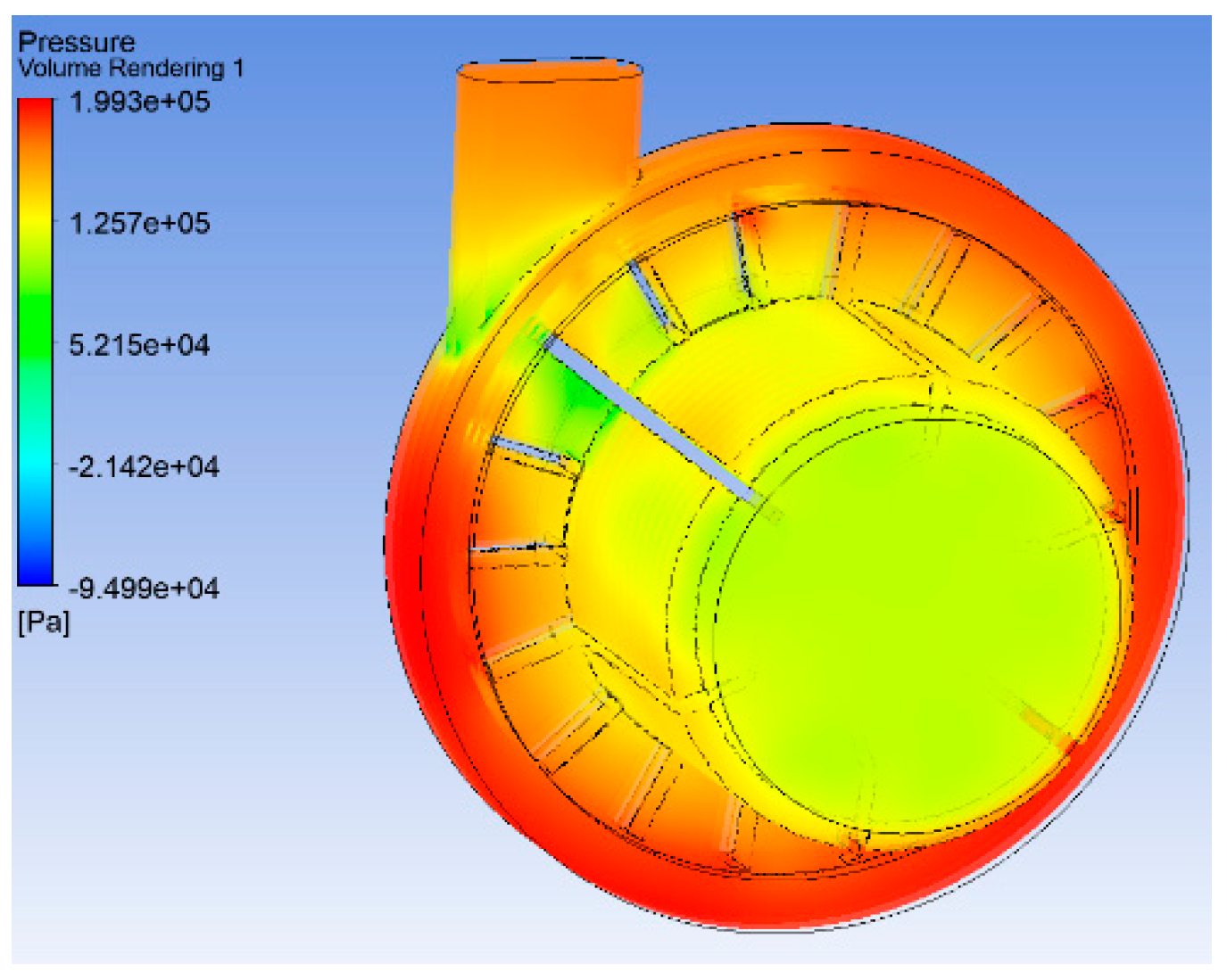
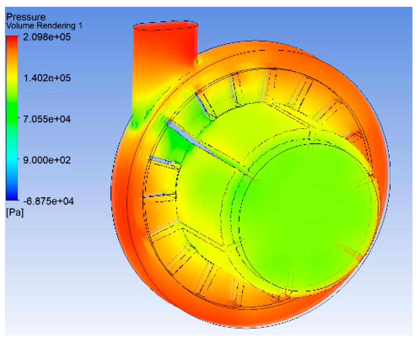
Figure 5,
Figure 6 and
Figure 7 show the pressure distribution of the liquid pumped by the rotor, according to the simulations.
Figure 5 shows the simulation for working point 4, as shown in
Table 1.
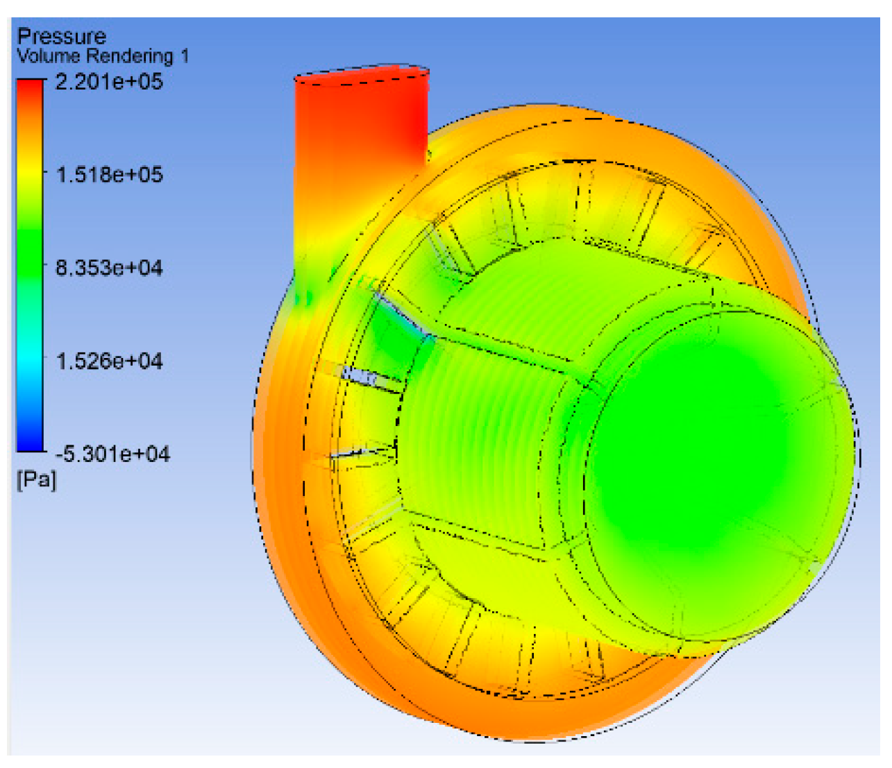
Figure 6 shows the simulation of operating point 5 and
Figure 7 shows the simulation for operating point 6 (as shown in
Table 1).
When the simulations were complete, positional tests were performed with the following assumptions: free liquid inlet to the pump from the main tank (control throttle “c” opening 100%); outlet pressure control by means of control damper “d”. The maximum pressure (
Figure 7) was small, approx. 1.2 bar (2.201 × 10
5 Pa) and it would have a low impact on the durability and sealing of the pump housing.
Figure 8 shows the rotor operation characteristics according to bench measurements. The data obtained during the simulation are also plotted in the graph.
As can be seen in
Figure 8, points of the simulation (red) coincide with the curve determined during the bench tests (black). For the first work point, the liquid volume flow rate is about 14% lower than that obtained in the bench tests. The numerical model was, therefore, found to reflect the actual rotor sufficiently to be used as the basis for further work. The relatively high flows without the rotor breaking the foam for pure liquid (water) suggested that when pumping a two-phase water/air mixture the pump would achieve the assumed capacities.
However, the lifting pressures obtained in bench tests were lower than expected. The pressures had to be adjusted downwards to obtain the appropriate mass flux (as in the tests), because during the simulation higher pressure was obtained at the inlet compared to the pressure during the bench tests. Therefore, the pressure was reduced by 0.1 bar. Using the criterion of similarity between the operating parameters of geometrically similar pumps (at the same rotational speed H1/H2 = (d1/d2)2 [
4,
24]), the rotor was, therefore, simulated again (3). The structural dimensions of the pump casing were not changed. The rotor diameter was increased by 10 mm (up to 180 mm). The internal blades of the rotor were extended by 10 mm (up to 35 mm). Simulations were performed for the new rotor geometry, corresponding to the process conditions of work point 2—i.e., p
2 = 1.0 bar and liquid volume flow
= 23.9 m
3/h.
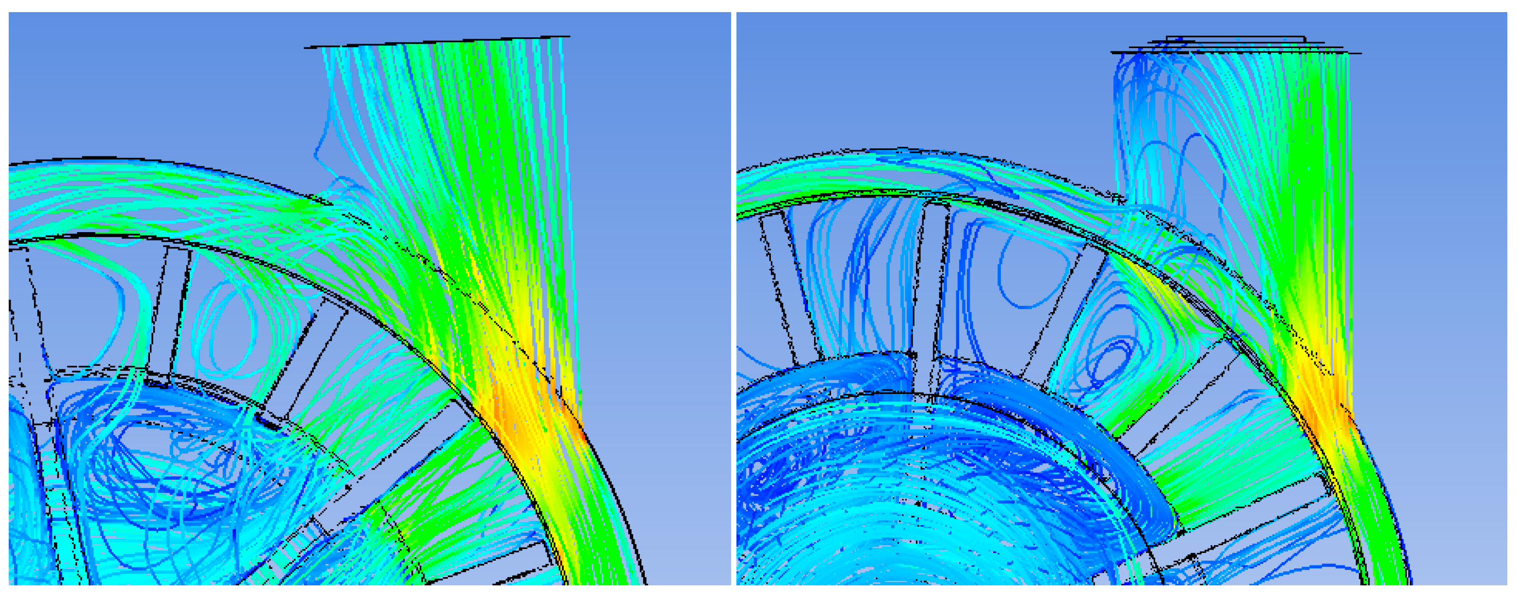
The simulations revealed that changing the rotor geometry had a negative impact on pump performance. Decreasing the distance between the wall of the pump chamber and the external diameter of the impeller caused disturbances in the liquid flow near the pump outlet port, as a result of which some of the liquid was driven back into the area of the impeller. This reduced the liquid output at the pump outlet (
Figure 9).
3.4. Computational Fluid Dynamics Simulations and Pump Bench Tests
Further tests were conducted to determine the operating parameters of the pump including all structural elements—i.e., pumping rotor, baffle plate, and breaking rotor. The calculation model assumed the presence of a water ring enabling the release of low-dispersion liquids into the discharge pipe and air flow into the foam chamber. The research was conducted in two stages. In the first stage, bench tests were performed; the second stage comprised verification of the CFD simulations. This sequence of tests was adopted due to the particularity of the device, in which flow and pressure do not clearly determine the operational performance of the pump. The purpose of the pump is to obtain liquid with the lowest possible share of gaseous phase in the discharge pipeline. Moreover, several tens of simulations would have been necessary to determine the potential characteristic work points (input parameters for numerical tests). Due to the limited possibilities for performing such large numbers of simulations, the reverse sequence of tests was adopted—i.e., bench tests were carried out which, on the basis of qualitative analysis of the degree of liquid dispersion at the pump outlet, enabled the identification of three distinct working points (low, intermediate, and high liquid dispersion at the outlet). The CFD simulations were then performed for the designated work points, providing graphical distributions of liquid flow through the impeller (3). This enabled the optimization of the flow, mainly thanks to visualization of the liquid ring created inside the rotor. Visualization allowed us to measure the ring thickness, the image of the two-phase mixture stream, and the distribution of individual liquid/gas phases in the entire rotor volume.
3.5. Bench Tests
The following assumptions were made for the positional conditions:
Clean water medium.
Free flow of liquid to the pump from the intermediate tank to the pump.
The water does not fill the entire section of the inlet stub.
The inflow is uneven.
Air enters the pump chamber.
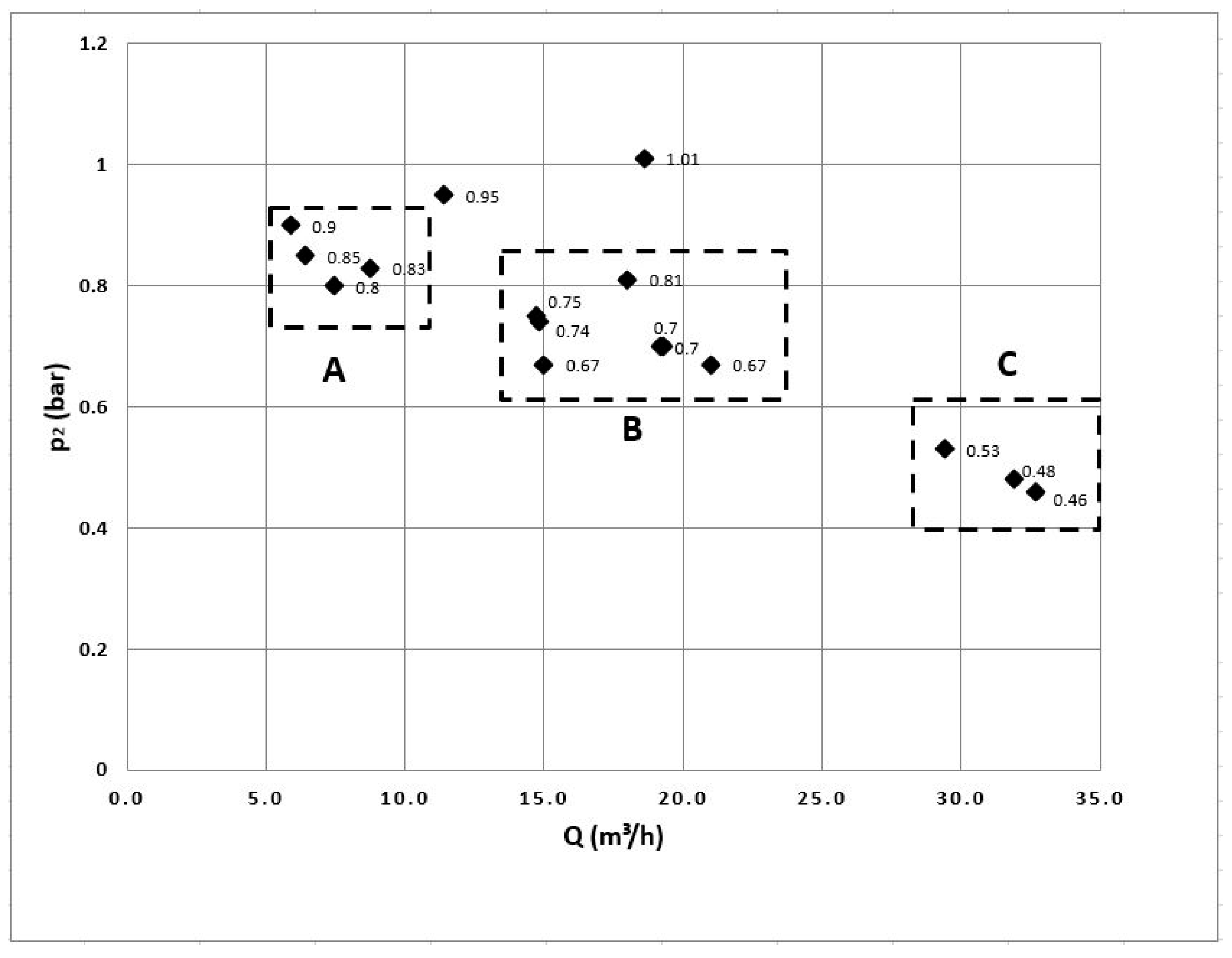
The supply of water was regulated by a throttle (c) in front of the intermediate tank, whereas the back pressure on the discharge pipeline was regulated by a throttle (d) behind the pump (
Figure 3). The results of the bench tests are presented in
Figure 10, where the working points p
2 = f(
). are shown by marking the degree of dispersion in each area.
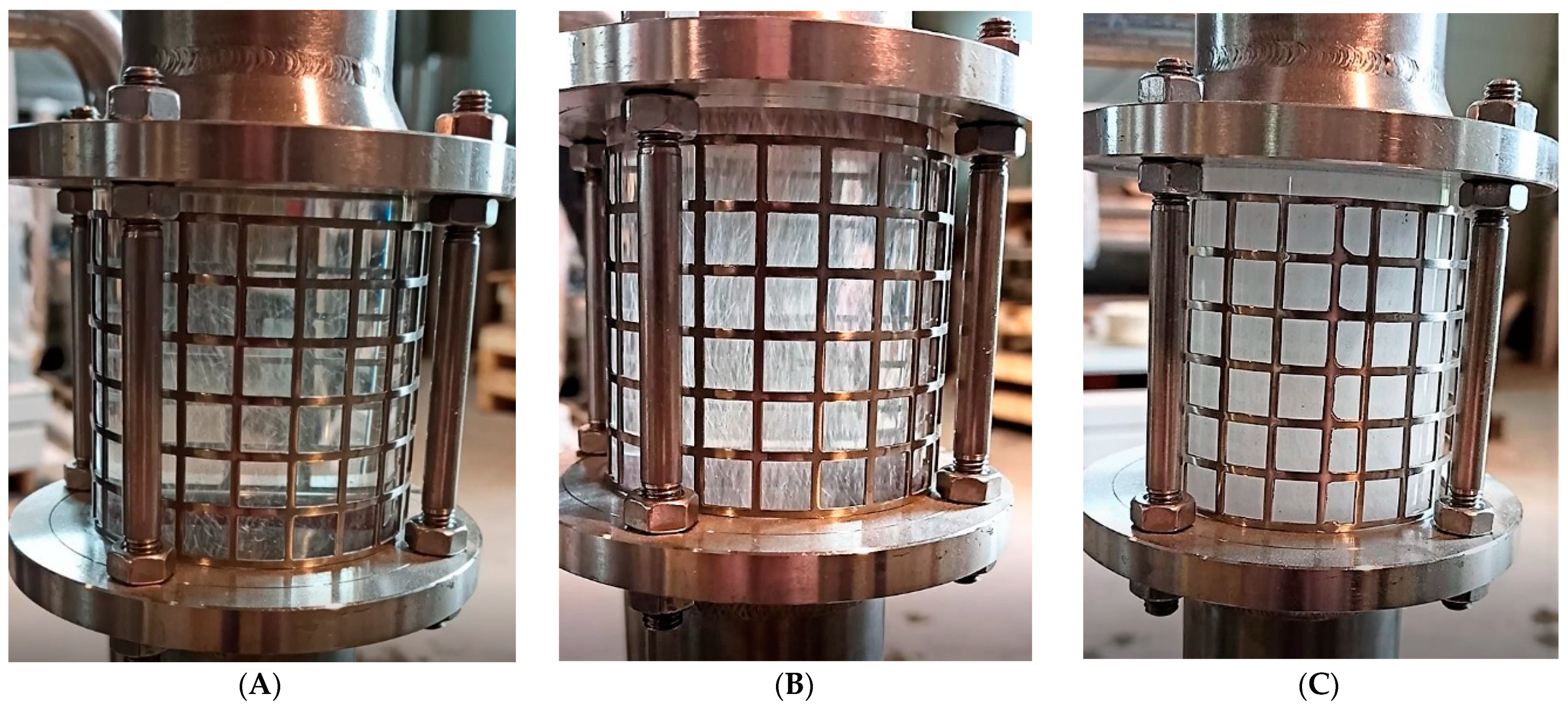
Figure 11 shows pictures of the liquid flow in the discharge pipeline for three selected parameters of the pump operation: (A)—low dispersion; (B)—intermediate dispersion; (C)—high dispersion.
As can be seen in
Figure 11, for each of the tested flows the two-phase mixture at the outlet from the stub pipe of the tested pump has a bubble structure, in which small gas bubbles are dispersed at a speed close to that of the liquid flowing upwards. The degree of dispersion of the liquid also varies, depending on the outlet back pressure of the pump. For low back pressure (p
2 = 0.4–0.6 bar), no water ring is formed in the impeller (3). This causes the outlet liquid to have a high degree of dispersion, whereas for back pressures in the range of p
2 = 0.8–0.9 bar the liquid has a low degree of dispersion.
4. Results and Discussion
Validation simulations were performed for three cases of liquid flow and dispersion (A, B, C), shown in
Figure 11, resulting from the assumed outlet pressure and liquid flow at the pump outlet. A 70/30 water/air mixture was assumed as the medium. The assumed inflow to the pump was similar to that in the bench tests, i.e., incomplete inlet cross-section (obscuration about 65%). Three series of simulations corresponding to three degrees of liquid dispersion were performed: SYM 1—low step, where p
2 = 0.85 bar and
= 7.1 m
3/h (average pressure and average mass flow of area A as shown in
Figure 12); SYM 2—intermediate step, where p
2 = 0.72 bar and
= 16.8 m
3/h (average pressure and average mass flow of area B as shown in
Figure 12); SYM 3—high step, where p
2 = 0.46 bar and
= 32.7 m
3/h. During the simulation for SYM 1 and SYM 2 it was necessary to correct pressure p
2: for SYM 1 from 0.85 bar to 0.75 bar and for SYM 2 from 0.79 bar to 0.70 bar.
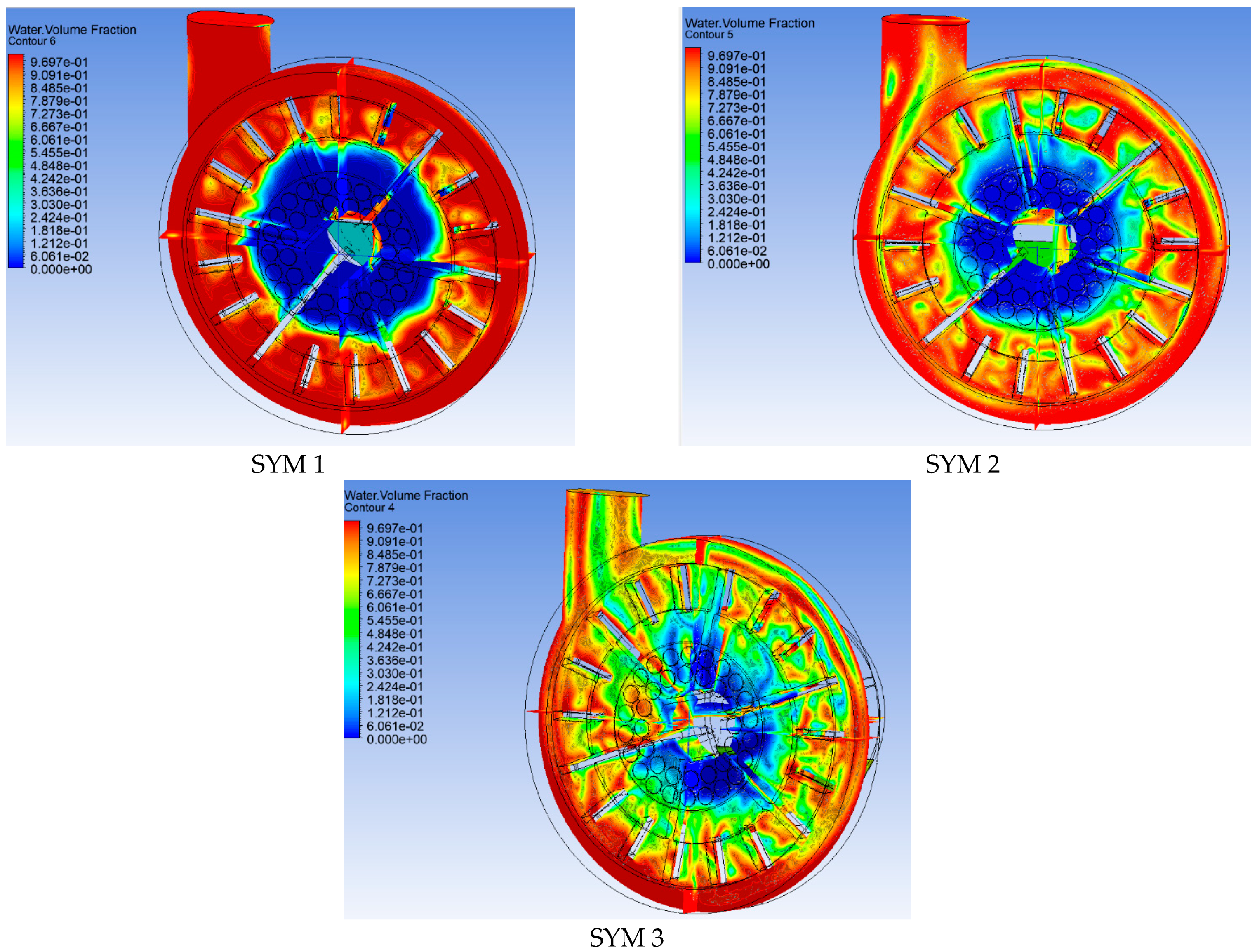
The results are collected in
Figure 12, which shows the water/air phase patterns from the view of the disc separating the pump chamber.
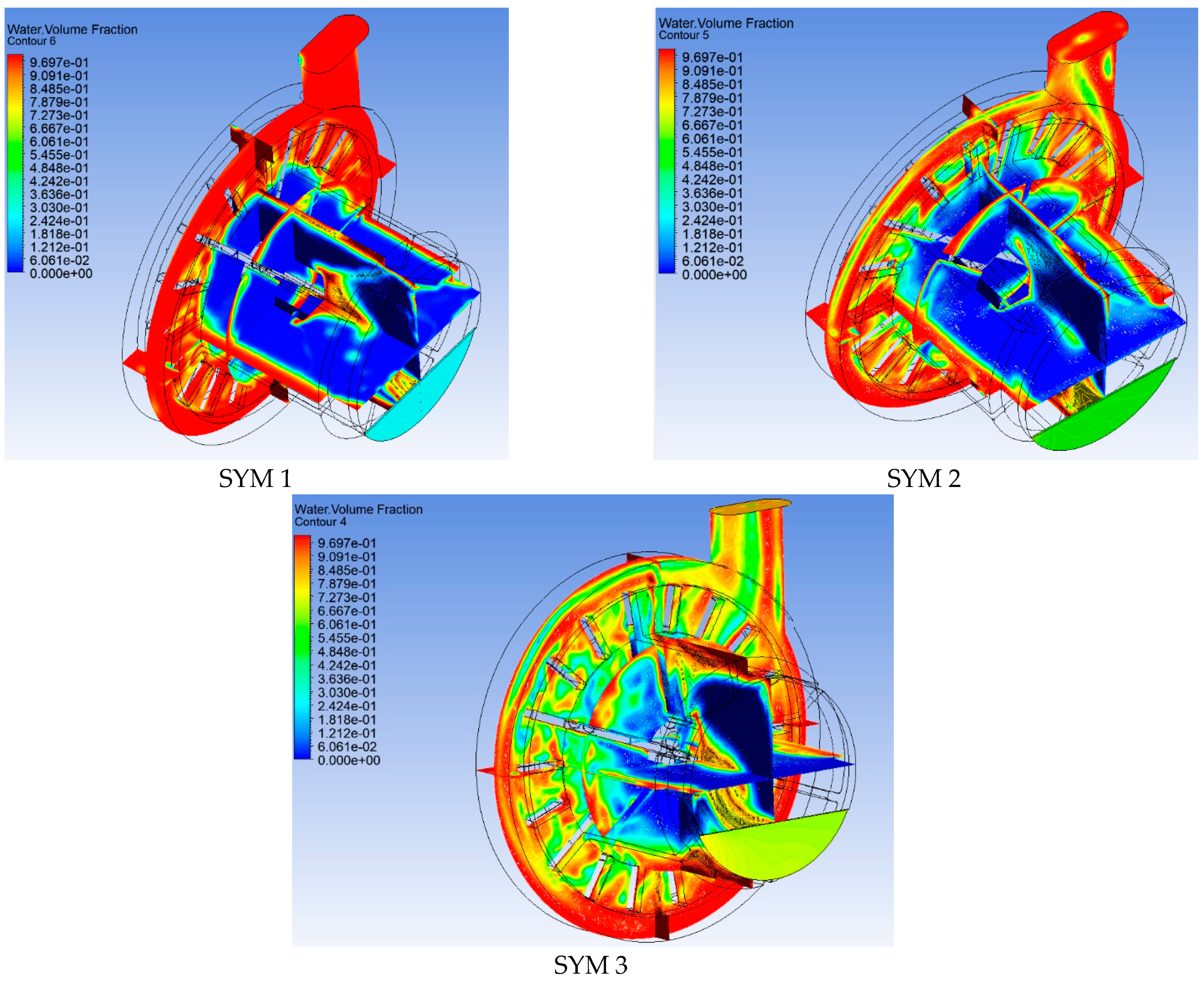
Figure 13 shows the phase patterns in the water ring and low-pressure zone. The zones of phase changes are marked with colors: red is 100% liquid, blue is 100% air.
A graphical representation of the amount of liquid and the backpressure affecting the degree of liquid dispersion was obtained on the basis of CFD analysis. Low flows and higher pressures ensure that a water ring forms on the outer diameters of the impeller and thus air accumulates near the pump axis, resulting in a high degree of phase separation. For SYM 1, almost 100% gaseous-free (air) liquid phase outflow was achieved at the pump outlet. Simulations show the influence of the geometry of the pump chamber dividing partition on the low-pressure zone (SYM 3). In the test case of a disc with two rows of holes, a large low-pressure zone is noticeable, and thus the thickness of the water ring is small. The thickness of the ring can be increased by raising the back pressure on the discharge, but then some of the liquid enters the foam breaking chamber, disturbing the process of pumping the liquid.
The results obtained during the simulation of the flows in the pump were compared with the results obtained during the experiments carried out on the test stand. The following power requirements were measured for the tested pump:
- (a).
For water pumping tests without a foam breaking impeller, the values were from N = 1.3 kW for = 15 m3/h to N = 2.5 kW for = 40.2 m3/h.
- (b).
For pumping a liquid-foam mixture, respectively from N = 1.1kW for area A (
Figure 10) to N = 1.6 kW for area C (
Figure 10).
The volumetric flow has been ranged from 6.0–9.0 m3/h (work area A) for the liquid-foam mixture (at the pump inlet) and foam-free liquid at the outlet port.
Due to the fact that the proposed solution has been innovative, and the issue of foam destruction was a complex problem that depended on various criteria. There were no comparative studies that allowed us to compare our results to other mechanical methods of foam separation and elimination. The use of mechanical foam separation allowed us to remove the chemical compounds responsible for the foam destruction. The mechanical method does not change the physicochemical properties of the liquid, and, therefore, the liquid’s tendency towards foam does not decrease.
5. Summary
This paper has presented simulation and bench test results for a special type of centrifugal pump, which enabled the transport of dispersive foaming liquids and simultaneous separation of the liquid phase. The results demonstrated a high correlation between the numerical model and the prototype of an innovative pump. The difference in flow through the pump of liquids with and without foam was demonstrated. The direct influence of the structure of the rotor and the foam destructor (number of holes) on the degree of liquid dispersion was also demonstrated. The number of holes determined the rate of liquid dispersion as well as the composition of the water ring in the rotor front within the low-pressure zone. The presented numerical model could be used as the basis for constructing other types of pumps, as well as for the optimization of the presented design.
Author Contributions
Conceptualization, T.P.O. and P.T.; methodology, E.S. and T.P.O.; software A.S., P.T.; validation, E.S., K.Ł. and T.P.O.; formal analysis, T.P.O. and E.S.; investigation, P.T. and A.S.; resources, A.O.; data curation, T.P.O.; writing—original draft preparation, T.P.O. and P.T.; writing—review and editing, E.S.; visualization, A.S.; supervision, T.P.O.; project administration, T.P.O. and E.S.; All authors have read and agreed to the published version of the manuscript.
Funding
This research was funded by the “Industrial Doctorate” project implemented at the Faculty of Biotechnology and Food Sciences of the Technical University of Lodz, contract No. 40/DW/2017/01/1, financed in the years 2017–2021 by Ministry of Science and Education.
Institutional Review Board Statement
Not applicable.
Informed Consent Statement
Not applicable.
Data Availability Statement
The data presented in this study are available on request from the corresponding author. The data are not publicly available due to the internal founding research of co-authors in their affiliation places.
Conflicts of Interest
The authors declare no conflict of interest.
Nomenclature
| volumetric flow rate, m3/h |
| mass flow, kg/s |
| p1 | inlet pressure, bar |
| p2 | outlet pressure, bar |
| ρ1 | water density, kg/m3 |
| ρ2 | air density, kg/m3 |
| N | electrical power, kW |
| n | rotation speed, min−1 |
References
- Pattison, R.C.; Baldea, M. Equation-oriented flowsheet simulation and optimization using pseudo-transient models. AlChE J. 2014, 60, 4104–4123. [Google Scholar] [CrossRef]
- Cui, T.; Ou, Y. Modeling of Scramjet Combustors Based on Model Migration and Process Similarity. Energies 2019, 12, 2516. [Google Scholar] [CrossRef]
- Dzikuć, M.; Kuryło, P.; Dudziak, R.; Szufa, S.; Dzikuć, M.; Godzisz, K. Selected Aspects of Combustion Optimization of Coal in Power Plants. Energies 2020, 13, 2208. [Google Scholar] [CrossRef]
- Seider, W.D.; Widagdo, S.; Seader, J.D.; Lewin, D.R. Perspectives on chemical product and process design. Comput. Chem. Eng. 2009, 33, 930–935. [Google Scholar] [CrossRef]
- Turton, R.; Bailie, R.C.; Whiting, W.B.; Shaeiwitz, J.A. Analysis, Synthesis and Design of Chemical Processes; Prentice Hall: Upper Saddle River, NJ, USA, 2008. [Google Scholar]
- Ławińska, K.; Szufa, S.; Obraniak, A.; Olejnik, T.; Siuda, R.; Kwiatek, J.; Ogrodowczyk, D. Disc Granulation Process of Carbonation Lime Mud as a Method of Post-Production Waste Management. Energies 2020, 13, 3419. [Google Scholar] [CrossRef]
- Motard, R.L.; Shacham, M.; Rosen, E.M. Steady state chemical process simulation. AlChE J. 1975, 21, 417–436. [Google Scholar] [CrossRef]
- Modrzewski, R.; Wodziński, P. Screens for segregation of mineral waste. Physicochem. Probl. 2011, 47, 267–274. [Google Scholar]
- Seider, W.D.; Seader, J.D.; Lewin, D.R.; Widagdo, S. Product & Design Principles: Synthesis, Analysis, and Evaluation, 4th ed.; John Wiley & Sons: Hoboken, NJ, USA, 2009; pp. 163–176. [Google Scholar]
- Olejnik, T.P. Milling kinetics of chosen rock materials under dry conditions considering strength and statistical properties of bed. Physicochem. Probl. 2011, 46, 145–154. [Google Scholar]
- Budych-Gorzna, M.; Szatkowska, B.; Jaroszynski, L.; Paulsrud, B.; Jankowska, E.; Jaroszynski, T.; Oleskowicz-Popiel, P. Towards an Energy Self-Sufficient Resource Recovery Facility by Improving Energy and Economic Balance of a Municipal WWTP with Chemically Enhanced Primary Treatment. Energies 2021, 14, 1445. [Google Scholar] [CrossRef]
- Akbaş, H.; Özdemir, G. An Integrated Prediction and Optimization Model of a Thermal Energy Production System in a Factory Producing Furniture Components. Energies 2020, 13, 5999. [Google Scholar] [CrossRef]
- Kyu Park, D.; Lee, Y. Numerical Simulations on the Application of a Closed-Loop Lake Water Heat Pump System in the Lake Soyang, Korea. Energies 2020, 13, 762. [Google Scholar] [CrossRef]
- Meshalkin, V.; Bobkov, V.; Dli, M.; Dovi, V. Optimization of Energy and Resource Efficiency in a Multistage Drying Process of Phosphate Pellets. Energies 2019, 12, 3376. [Google Scholar] [CrossRef]
- Sargent, R.W.H. Applications of an electronic digital computer in the design of low temperature plant. Trans. Instit. Chem. Eng. 1958, 36, 201–214. [Google Scholar]
- Grossmann, I.E.; Sargent, R.W.H. Optimum design of heat exchanger networks. Comput. Chem. Eng. 1978, 2, 1–7. [Google Scholar] [CrossRef]
- Moin, P.; Kim, J. Numerical investigation of turbulent channel flow. J. Fluid Mech. 1982, 118, 341–377. [Google Scholar] [CrossRef]
- Sargent, R.W.H. Forecasts and trends in systems engineering. Chem. Eng. 1972, 262, 226–230. [Google Scholar]
- Kryszak, D.; Bartoszewicz, A.; Szufa, S.; Piersa, P.; Obraniak, A.; Olejnik, T.P. Modeling of Transport of Loose Products with the Use of the Non-Grid Method of Discrete Elements (DEM). Processes 2020, 8, 1489. [Google Scholar] [CrossRef]
- Biegler, L.T. Nonlinear Programming: Concepts, Algorithms, and Applications to Chemical Processes; SIAM: Philadelphia, PA, USA, 2010. [Google Scholar]
- Dowling, A.W.; Biegler, L.T. A framework for efficient large scale equation-oriented flowsheet optimization. Comput. Chem. Eng. 2015, 72, 3–20. [Google Scholar] [CrossRef]
- Edgar, T.F.; Himmelblau, D.M.; Lasdon, L.S. Optimization of Chemical Processes; McGraw-Hill: New York, NY, USA, 2001. [Google Scholar]
- Grossmann, I.E.; Apap, R.M.; Calfa, B.A.; Garcia-Herreros, P.; Zhang, Q. Recent advances in mathematical programming techniques for the optimization of process systems under uncertainty. Comput. Chem. Eng. 2016, 91, 3–14. [Google Scholar] [CrossRef]
- Shacham, M.; Macchieto, S.; Stutzman, L.F.; Babcock, P. Equation oriented approach to process flowsheeting. Comput. Chem. Eng. 1982, 6, 79–95. [Google Scholar] [CrossRef]
- Tsay, C.; Pattison, R.C.; Baldea, M. A pseudo-transient optimization framework for periodic processes: Pressure swing adsorption and simulated moving bed chromatography. AlChE J. 2017. [Google Scholar] [CrossRef]
- Exerowa, D.; Kruglyakov, P.M. Foam and Foam Films: Theory, Experiment, Application; Elsevier: Amsterdam, The Netherlands, 1998; pp. 22–30. [Google Scholar]
- Winterburn, J. Sound Methods of Breaking Foam. Fourth Year Project Report-Engineering Science, Finals Part II; Pembroke College: Cambridge, UK, 2007. [Google Scholar]
- Garrett, P.R. Defoaming: Antifoams and mechanical methods. Curr. Opin. Colloid Interface Sci. 2015, 20, 81–91. [Google Scholar] [CrossRef]
- Rodríguez, G.; Riera, E.; Gallego-Juárez, J.A.; Acosta, V.M.; Pinto, A.; Martínez, I.; Blanco, A. Experimental study of defoaming by air-borne power ultrasonic technology. Phys. Procedia 2010, 3, 135–139. [Google Scholar] [CrossRef]
- Janczar-Smuga, M.; Pietkiewicz, J.J.; Bogacz-Radomska, L. Problems with foam occurrence in the beet processing by the sugar production biotechnology. Res. Pap. Wrocław Univ. Econ. 2008, 30, 139–141. [Google Scholar]
- Erasmus, A. Bursting the Bubbles. Potato Processing. Available online: https://www.potatobusiness.com/process/bursting-the-bubbles/ (accessed on 22 January 2021).
- Gélinas, P. Aeration and Foam Control in Baker’s Yeast Production: Mapping Patents. Compr. Rev. Food Sci. Food Saf. 2016, 15. [Google Scholar] [CrossRef] [PubMed]
- Garrett, P.R. Defoaming: Theory and Industrial Applications; CRC Press/Taylor and Francis Group: Boca Raton, FL, USA, 1992; pp. 221–268. [Google Scholar]
- Exerowa, D.; Gochev, G.; Platikanov, D.; Liggieri, L.; Miller, R. Foam Films and Foams: Fundamentals and Applications; CRC Press: Boca Raton, FL, USA, 2018; pp. 77–98. [Google Scholar]
- Karakashev, S.I.; Grozdanova, M.V. Foams and antifoams. Adv. Colloid Interface Sci. 2012, 176–177, 1–17. [Google Scholar] [CrossRef] [PubMed]
- Sulzer. AHLSTAR End Suction Single Stage Centrifugal Pumps. Personal communication, 2020. [Google Scholar]
- Davidson, L. Fluid Mechanics, Turbulent Flow and Turbulence Modelling; Chalmers University of Technology: Göteborg, Sweden, 2020; pp. 81–90. [Google Scholar]
- Wilcox, D.C. Turbulence Modeling for CFD, 3rd ed.; DCW Industries: La Canada, CA, USA, 2006; ISBN 1928729088. [Google Scholar]
- ANSYS Inc. ANSYS Fluent Theory Guide; Release 15.0; ANSYS Inc.: Canonsburg, PA, USA, 2013; pp. 51–57. [Google Scholar]
- Xian-hua, L.; Shu-jia, Z.; Bao-lin, Z.; Qing-bo, H. The study of the k-ε turbulence model for numerical simulation of centrifugal pump. In Proceedings of the 7th International Conference on Computer-Aided Industrial Design and Conceptual Design, Hangzhou, China, 17–19 November 2006. [Google Scholar]
- Mendoza-Escamilla, V.X.; Alonzo-García, A.; Mollinedo, H.R.; González-Neria, I.; Yáñez-Varela, J.A.; Martinez-Delgadillo, S.A. Assessment of k–ε models using tetrahedral grids to describe the turbulent flow field of a PBT impeller and validation through the PIV technique. Chin. J. Chem. Eng. 2018, 26, 942–956. [Google Scholar] [CrossRef]
- Shashi Kumar, S.; Prakash, K.A. An RNG based k-epsilon turbulence model using the realizable eddy viscosity formulation. In Proceedings of the 14th European Turbulence Conference, Lyon, France, 1–4 September 2013. [Google Scholar]
- Sosnowski, M.; Krzywański, J.; Gnatowska, R. Polyhedral meshing as an innovative approach to computational domain discretization of a cyclone in a fluidized bed CLC unit. Energy Fuels 2016 EPJ Web Conf. 2018, 180, 02096. [Google Scholar] [CrossRef]
- Stępniewski, M. Pumps; WNT: Warszawa, Poland, 1978; pp. 195–197. [Google Scholar]
Figure 1.
Schematic diagram of the skimming pump: 1—casing; 2—baffle plate; 3—liquid pumping rotor; 4—foam breaking rotor.
Figure 1.
Schematic diagram of the skimming pump: 1—casing; 2—baffle plate; 3—liquid pumping rotor; 4—foam breaking rotor.
Figure 2.
Axionometric drawing of the tested pump: 1—casing; 2—baffle plate; 3—liquid pumping rotor; 4—foam breaking rotor.
Figure 2.
Axionometric drawing of the tested pump: 1—casing; 2—baffle plate; 3—liquid pumping rotor; 4—foam breaking rotor.
Figure 3.
Components of the test stand: a—main tank; b—intermediate tank; c, d—control throttle; e—pipe sight glass; p1, p2—pressure sensors; —flow meter.
Figure 3.
Components of the test stand: a—main tank; b—intermediate tank; c, d—control throttle; e—pipe sight glass; p1, p2—pressure sensors; —flow meter.
Figure 4.
View of the test stand; (a)—general vie of the stand, (b)—pump section, (c)—measuring devices.
Figure 4.
View of the test stand; (a)—general vie of the stand, (b)—pump section, (c)—measuring devices.
Figure 5.
Pressure schedules of the pumped liquid for simulation 4.
Figure 5.
Pressure schedules of the pumped liquid for simulation 4.
Figure 6.
Pressure schedules of the pumped liquid for simulation 5.
Figure 6.
Pressure schedules of the pumped liquid for simulation 5.
Figure 7.
Pressure schedules of the pumped liquid for simulation 6.
Figure 7.
Pressure schedules of the pumped liquid for simulation 6.
Figure 8.
Diagram of changes in lifting height p2 as a function of pump volume flow in the impeller bench test.
Figure 8.
Diagram of changes in lifting height p2 as a function of pump volume flow in the impeller bench test.
Figure 9.
Liquid jet profiles in the area of the pump outlet port for both impeller designs: primary impeller (left), impeller with larger diameter (right).
Figure 9.
Liquid jet profiles in the area of the pump outlet port for both impeller designs: primary impeller (left), impeller with larger diameter (right).
Figure 10.
Results of the pump station tests. Working points p2 = f() show the degree of dispersion in areas A, B, and C.
Figure 10.
Results of the pump station tests. Working points p2 = f() show the degree of dispersion in areas A, B, and C.
Figure 11.
Liquid images for three two-phase flow conditions. (A)—low dispersion; (B)—intermediate dispersion; (C)—high dispersion.
Figure 11.
Liquid images for three two-phase flow conditions. (A)—low dispersion; (B)—intermediate dispersion; (C)—high dispersion.
Figure 12.
View from the separating disc of the pump chamber; (SYM 1), (SYM 2), (SYM 3).
Figure 12.
View from the separating disc of the pump chamber; (SYM 1), (SYM 2), (SYM 3).
Figure 13.
View from the rotor front with low pressure zone and water ring; (SYM 1), (SYM 2), (SYM 3).
Figure 13.
View from the rotor front with low pressure zone and water ring; (SYM 1), (SYM 2), (SYM 3).
Table 1.
List of parameters used in the calculation model.
Table 1.
List of parameters used in the calculation model.
| Simulation/Working Point |
|---|
| Parameter | 1 | 2 | 3 | 4 | 5 | 6 |
|---|
| p1, bar | 0.1 | 0.1 | 0.1 | 0.1 | 0.1 | 0.1 |
| p2, bar | 0.7 | 0.8 | 0.9 | 1.0 | 1.1 | 1.2 |
| , m3/h | 30.8 | 29.4 | 26.7 | 23.9 | 18.6 | 15.3 |
| , kg/s | 8.55 | 8.16 | 7.41 | 6.63 | 5.15 | 4.25 |
| Publisher’s Note: MDPI stays neutral with regard to jurisdictional claims in published maps and institutional affiliations. |
© 2021 by the authors. Licensee MDPI, Basel, Switzerland. This article is an open access article distributed under the terms and conditions of the Creative Commons Attribution (CC BY) license (http://creativecommons.org/licenses/by/4.0/).


 ,
, 


