
Measurement of Static Frequency Characteristics of Home Appliances in Smart Grid Systems

 , ,
, ,  , , , and
Abstract
1. Introduction
Literature Review
2. Measurement and Data Analysis
- General categorization:
- ○
- resistive loads (R);
- ○
- motoric loads (M);
- ○
- loads with electronic ballast (EB);
- ○
- loads with magnetic ballast (MB).
- Light sources:
- ○
- light sources with magnetic ballast (LM);
- ○
- light sources with electronic ballast (LE);
- ○
- resistive light sources (LR).
2.1. Measurement
2.2. Data Analysis
3. Measurement Results
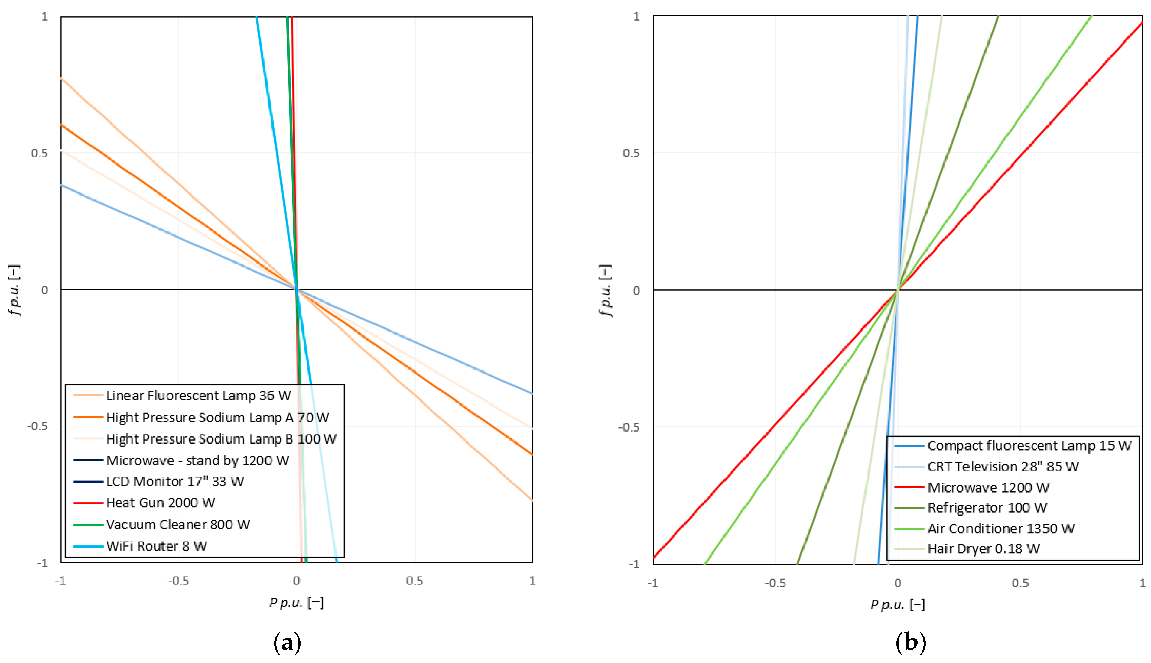
- positive: KP > 0.01;
- negative: KP < −0.01;
- no effect (negligible): −0.01 ≤ KP ≤ 0.01.
Discussion on Measurement Results
- Measurement methodology:
- ○
- frequency range (minimum proposed range between 47.5 and 51.5 Hz due to requirements on generating modules [45]);
- ○
- equipment stabilization (e.g., thermal, …).
- Defined operating conditions of the device:
- ○
- stand-by mode;
- ○
- no-load;
- ○
- load level (average, max, …).
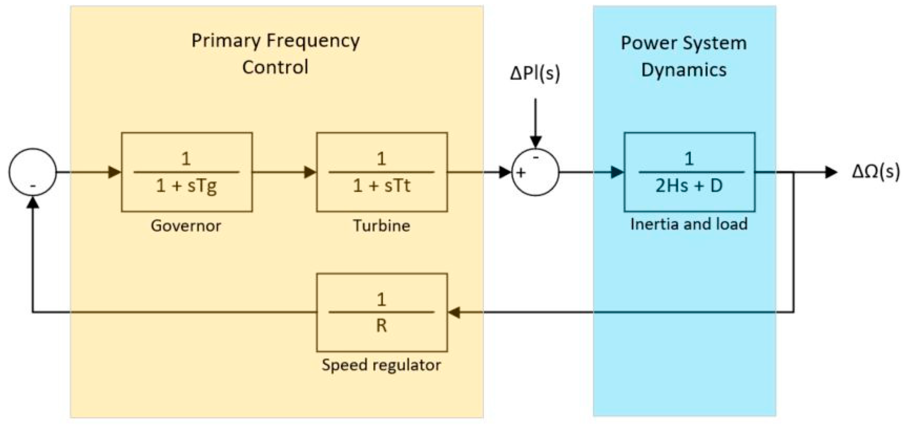
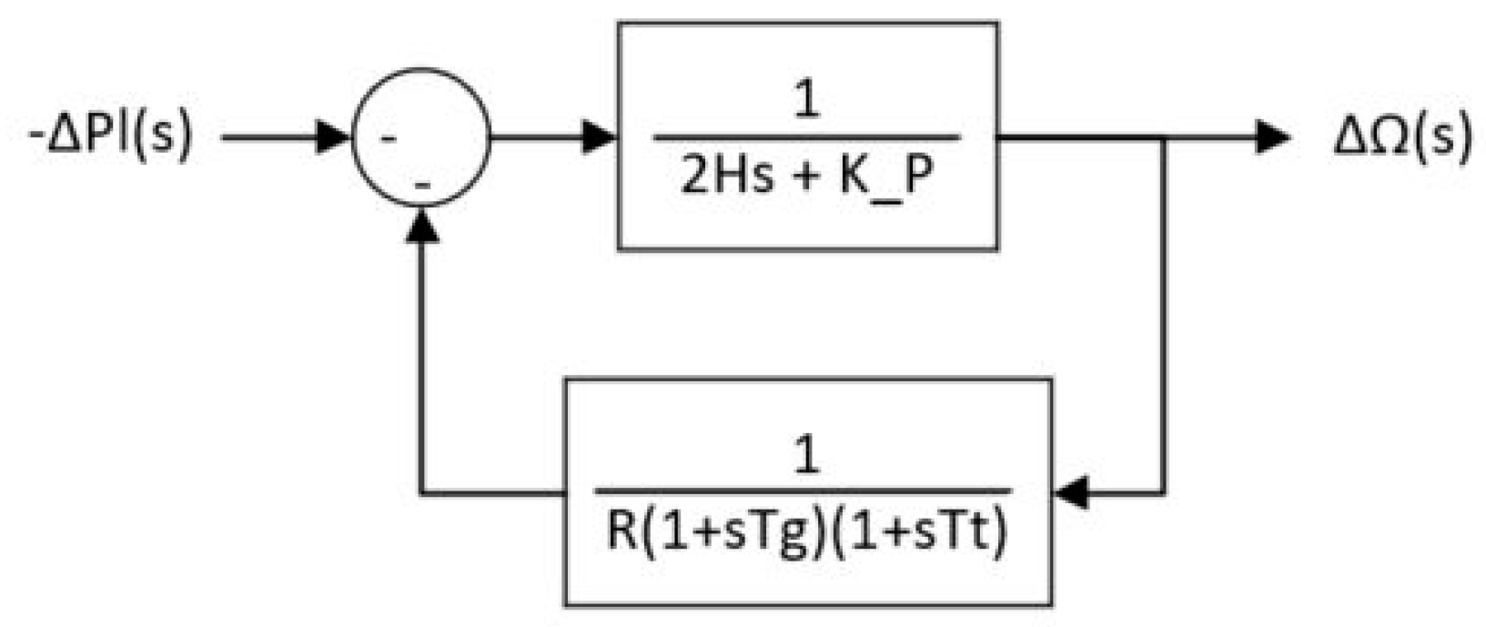
4. Impact of Measured Loads on Frequency Control in Island Operation
- turbine time constant (Tt) = 0.5 s;
- governor time constant (Tg) = 0.2 s;
- governor speed regulator (droop characteristic) (R) = 5%;
- inertia time constant (H) = 5 s;
- damping constant (D) (or KP for load—measured device);
- power load change (ΔPl) = −10% (generation outage).
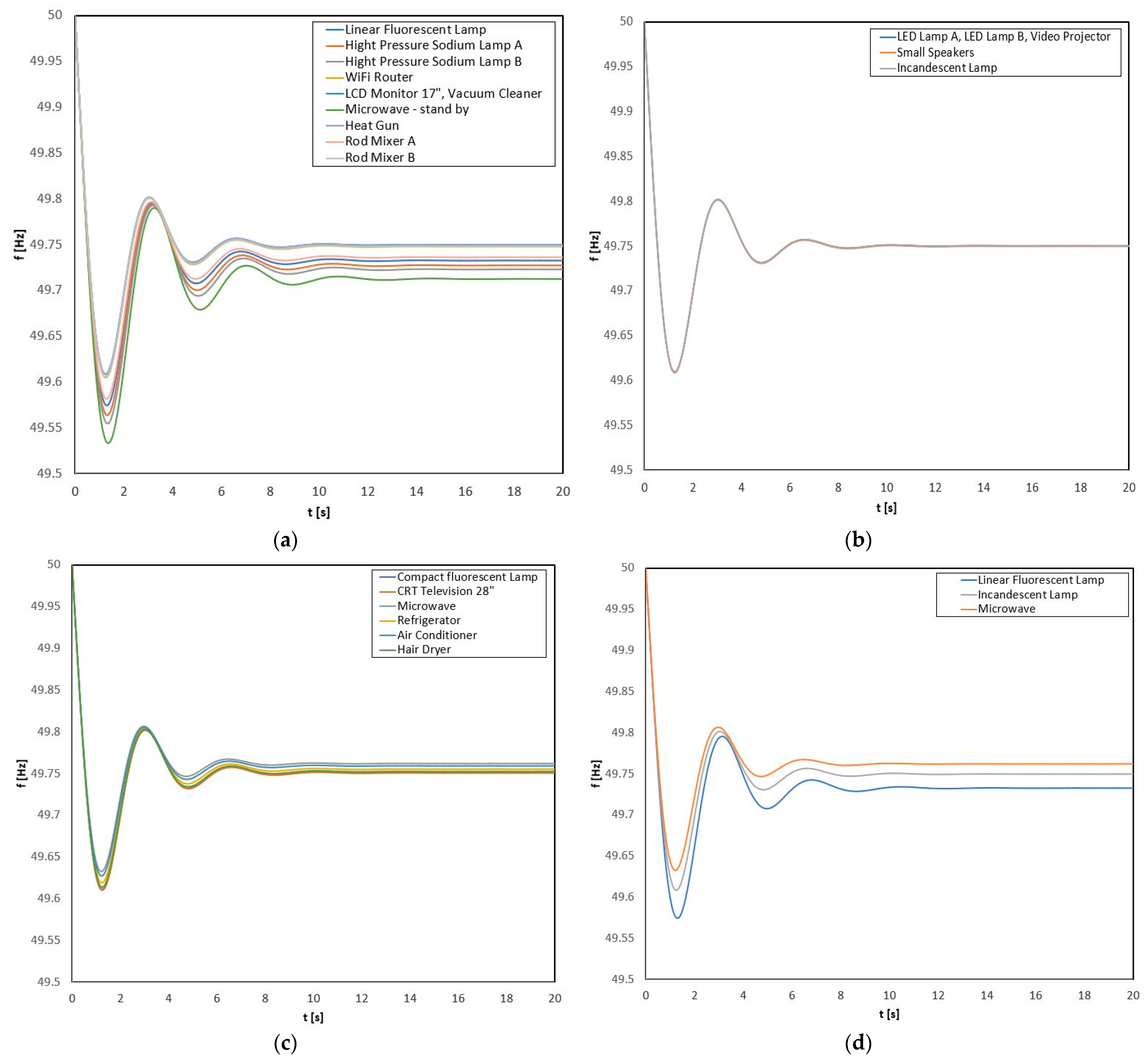
4.1. Discussion on Simulation Results
- maximum (dynamic) frequency deviation (Δfmax);
- quasi-stationary deviation (Δf).
4.2. Concerning Further Smart Grid Possibilities
5. Conclusions
- identification and organization of more data of household appliances in more detail and, if possible, creation of common data groups so that that load group composition may be estimated more easily and reliably;
- measurement of static load characteristics of a wider group of the same type of devices (improvement of current statistics and addition of new types of loads);
- measurement of static characteristics of three-phase devices (a wider group of devices);
- analysis of the frequency response in island operation concerning a larger number of devices with different frequency sensitivity coefficients;
- focusing on devices with reactive power consumption—the operating impedance is frequency-dependent.
Author Contributions
Funding
Institutional Review Board Statement
Informed Consent Statement
Data Availability Statement
Acknowledgments
Conflicts of Interest
References
- Hoballah, A. Power System Stability Assessment and Enhancement Using Computational Intelligence; Universität Duisburg-Essen: Duisburg, Germany, 2011. [Google Scholar]
- Machowski, J.; Lubosny, Z.; Bialek, J.W.; Bumby, J.R. Power System Dynamics: Stability and Control; John Wiley & Sons: Hoboken, NJ, USA, 2020; ISBN 978-1-119-52634-6. [Google Scholar]
- Kundur, P. Power System Stability and Control; McGraw-Hill: New York, NY, USA, 1994; ISBN 978-0-07-063515-9. [Google Scholar]
- Shenkman, A.L. Transient Analysis of Electric Power Circuits Handbook; Springer Science & Business Media: New York, NY, USA, 2006; ISBN 978-0-387-28799-7. [Google Scholar]
- Load Representation for Dynamic Performance Analysis (of Power Systems). IEEE Trans. Power Syst. 1993, 8, 472–482. [CrossRef]
- Concordia, C.; Ihara, S. Load Representation in Power System Stability Studies. IEEE Trans. Power Appar. Syst. 1982, PAS-101, 969–977. [Google Scholar] [CrossRef]
- O’Sullivan, J.; Power, M.; Flynn, M.; O’Malley, M. Modelling of Frequency Control in an Island System. In Proceedings of the IEEE Power Engineering Society 1999 Winter Meeting (Cat. No.99CH36233), New York, NY, USA, 31 January–4 February 1999; Volume 1, pp. 574–579. [Google Scholar]
- Omara, H. A Methodology for Determining the Load Frequency Sensitivity. Ph.D. Thesis, The University of Manchester, Manchester, UK, 2012. [Google Scholar]
- Azizan, A.R.B. Simulation of Dynamic Load Effect on Power System; Universiti Tun Hussein Onn Malaysia: Parit Raja, Malaysia, 2013. [Google Scholar]
- Abhyankar, S.; Balasubramaniam, K.; Cui, B. Load Model Parameter Estimation by Transmission-Distribution Co-Simulation. In Proceedings of the Power Systems Computation Conference (PSCC), Dublin, Ireland, 11–15 June 2018; pp. 1–7. [Google Scholar]
- Bevrani, H.; Shafiee, Q.; Golpira, H.; Taczi, I.; Hartmann, B.; Vokony, I.; Lak, M.; Aragon, E.; Johnson, A.; Russell, B.; et al. Smart Grid and Stability of Power Systems; IEEE Smart Grid Recource Center: New York, NY, USA, 2019. [Google Scholar]
- Sabbir, K.G.; Kashem, M.A.; Negnevitsky, M. Response Analysis of Large Induction Motors at Different Voltages and Frequencies. In Proceedings of the Australasian Universities Power Engineering Conference (AUPEC 2006), Melbourne, Australia, 10–13 December 2006. [Google Scholar]
- Chen, Q.; Jiang, M.; Ju, P.; Shan, X.; Wang, B.; Wang, Y.; Yu, F.; Xu, L.; Qin, C. Frequency Characteristic of New-Type Load Considering Power Electronics Technology. In Proceedings of the IEEE 7th Annual International Conference on CYBER Technology in Automation, Control, and Intelligent Systems (CYBER), Honolulu HI, USA, 31 July–4 August 2017; pp. 730–734. [Google Scholar]
- Davidson, J.; Ringwood, J.V. Mathematical Modelling of Mooring Systems for Wave Energy Converters—A Review. Energies 2017, 10, 666. [Google Scholar] [CrossRef]
- Lindén, K.; Segerqvist, I. Modelling of Load Devices and Studying Load/System Characteristics; School of Electrical and Computer Engineering, Chalmers University of Technology: Göteborg, Sweden, 1993. [Google Scholar]
- Yamashita, K.; Djokic, S.; Matevosyan, J.; Resende, F.O.; Korunovic, L.M.; Dong, Z.Y.; Milanovic, J.V. Modelling and Aggregation of Loads in Flexible Power Networks—Scope and Status of the Work of CIGRE WG C4.605. IFAC Proc. Vol. 2012, 45, 405–410. [Google Scholar] [CrossRef]
- Wang, Q.; Zhao, B.; Tang, Y.; Liu, L.-P. Modeling of Load Frequency Characteristics in the Load Model for Power System Digital Simulation. In Proceedings of the IEEE 7th Annual International Conference on CYBER Technology in Automation, Control, and Intelligent Systems (CYBER), Honolulu, HI, USA, 31 July–4 August 2017; pp. 538–542. [Google Scholar]
- Changchun, C.; Yuqing, J.; Yiping, Y.; Ping, J. Load Modeling with Considering Frequency Characteristic. In Proceedings of the International Conference on Sustainable Power Generation and Supply (SUPERGEN 2012), Hangzhou, China, 8–9 September 2012; pp. 1–6. [Google Scholar]
- Yamashita, K.; Asada, M.; Yoshimura, K. A Development of Dynamic Load Model Parameter Derivation Method. In Proceedings of the IEEE Power Energy Society General Meeting, Calgary, AB, Canada, 26–30 July 2009; pp. 1–8. [Google Scholar]
- Lian, H.; Di, X.; Shen, Z.; Feng, M. Detailed Power Distribution Network Planning Based on the Description of Load Characteristics. In Proceedings of the China International Conference on Electricity Distribution (CICED), Shenzhen, China, 23–26 September 2014; pp. 1759–1762. [Google Scholar]
- Diao, Y.; Liu, K.; Hu, L.; Jia, D.; Dong, W. Classification of Massive User Load Characteristics in Distribution Network Based on Agglomerative Hierarchical Algorithm. In Proceedings of the International Conference on Cyber-Enabled Distributed Computing and Knowledge Discovery (CyberC), Chengdu, China, 13–15 October 2016; pp. 169–172. [Google Scholar]
- Chen, C.; Su, C.; Teng, J. Determination of Load Characteristics for Electrical Load Analysis in Shipboard Microgrids. In Proceedings of the IEEE/IAS 55th Industrial and Commercial Power Systems Technical Conference (I CPS), Calgary, AB, Canada, 5–8 May 2019; pp. 1–9. [Google Scholar]
- IEC Smart Grid Standardization Roadmap. Available online: https://www.iec.ch/smartgrid/downloads/sg3_roadmap.pdf (accessed on 9 July 2020).
- Zhang, Q.; Guo, Q.; Yu, Y. Research on the Load Characteristics of Inverter and Constant Speed Air Conditioner and the Influence on Distribution Network. In Proceedings of the China International Conference on Electricity Distribution (CICED), Xi’an, China, 10–13 August 2016; pp. 1–4. [Google Scholar]
- Gong, C.; Zhang, B.; Ding, Y.; Ma, L.; Zhao, Y.; Li, X. Operating Characteristics and Influence on Power Grid with Distributed Electric Heating Considering Load Transfer. In Proceedings of the 2nd IEEE Conference on Energy Internet and Energy System Integration (EI2), Beijing, China, 20–22 October 2018; pp. 1–4. [Google Scholar]
- Hou, P.; Wang, J.; Xu, Y.; Huang, K.; Li, J. Research on the Dynamic Characteristics of Microgrid with Pulsed Nonlinear Load. In Proceedings of the IEEE 8th International Power Electronics and Motion Control Conference (IPEMC-ECCE Asia), Hefei, China, 22–25 May 2016; pp. 1732–1736. [Google Scholar]
- Yang, Y.; Liu, G.; Yang, Z.; Fan, S. A Study of Load Characteristic of the Building Heating and Cooling System in Smart Distribution Grid. In Proceedings of the China International Conference on Electricity Distribution (CICED), Shenzhen, China, 23–26 September 2014; pp. 928–932. [Google Scholar]
- Huang, H.; Li, F. Sensitivity Analysis of Load-Damping Characteristic in Power System Frequency Regulation. IEEE Trans. Power Syst. 2013, 28, 1324–1335. [Google Scholar] [CrossRef]
- Liao, S.; Xu, J.; Sun, Y.; Gao, W.; Ma, X.-Y.; Zhou, M.; Qu, Y.; Li, X.; Gu, J.; Dong, J. Load-Damping Characteristic Control Method in an Isolated Power System With Industrial Voltage-Sensitive Load. IEEE Trans. Power Syst. 2016. [CrossRef]
- Obaid, Z.A.; Cipcigan, L.M.; Abrahim, L.; Muhssin, M.T. Frequency Control of Future Power Systems: Reviewing and Evaluating Challenges and New Control Methods. J. Mod. Power Syst. Clean Energy 2019, 7, 9–25. [Google Scholar] [CrossRef]
- Popa, G.N.; Iagăr, A.; Diniș, C.M. Considerations on Current and Voltage Unbalance of Nonlinear Loads in Residential and Educational Sectors. Energies 2021, 14, 102. [Google Scholar] [CrossRef]
- Saeed Uz Zaman, M.; Irfan, M.; Ahmad, M.; Mazzara, M.; Kim, C.-H. Modeling the Impact of Modified Inertia Coefficient (H) Due to ESS in Power System Frequency Response Analysis. Energies 2020, 13, 902. [Google Scholar] [CrossRef]
- Järventausta, P.; Repo, S.; Rautiainen, A.; Partanen, J. Smart Grid Power System Control in Distributed Generation Environment. IFAC Proc. Vol. 2009, 42, 10–19. [Google Scholar] [CrossRef]
- Steinhart, C.J.; Gratza, M.; Kerber, G.; Finkel, M.; Witzmann, R. Determination of Load-Frequency Dependence in Island Power Supply. CIRED—Open Access Proc. J. 2017, 2017, 1031–1034. [Google Scholar] [CrossRef][Green Version]
- Ulbig, A.; Borsche, T.S.; Andersson, G. Impact of Low Rotational Inertia on Power System Stability and Operation. IFAC Proc. Vol. 2014, 47, 7290–7297. [Google Scholar] [CrossRef]
- Ye, L.; Baohui, Z.; Tingyue, T.; Zhe, G. Influence of Load Characteristics on System Dynamics and Load-Shedding Control Effects in Power Grid. In Proceedings of the 27th Chinese Control and Decision Conference (2015 CCDC), Qingdao, China, 22–25 May 2015; pp. 5160–5163. [Google Scholar]
- Bracinik, P.; Latkova, M.; Altus, J. Retrofit of Distributed Generation vs. Frequency Control in Smart Grids at Overfrequency. Electr. Eng. 2017, 99, 1403–1415. [Google Scholar] [CrossRef]
- Kanálik, M.; Margitová, A.; Dolník, B.; Medved’, D.; Pavlík, M.; Zbojovský, J. Analysis of Low-Frequency Oscillations of Electrical Quantities during a Real Black-Start Test in Slovakia. Int. J. Electr. Power Energy Syst. 2021, 124, 106370. [Google Scholar] [CrossRef]
- Vengatesh, R.P.; Rajan, S.E.; Sivaprakash, A. An Intelligent Approach for Dynamic Load Frequency Control with Hybrid Energy Storage System. Aust. J. Electr. Electron. Eng. 2019, 16, 266–275. [Google Scholar] [CrossRef]
- Vrana, M.; Drapela, J.; Topolanek, D.; Vycital, V.; Jurik, M.; Blahusek, R.; Kurfirt, M. Battery Storage and Charging Systems Power Control Supporting Voltage in Charging Mode. In Proceedings of the 19th International Conference on Harmonics and Quality of Power (ichqp), Dubai, United Arab Emirates, 6–7 July 2020; IEEE: New York, NY, USA, 2020; ISBN 978-1-72813-697-4. [Google Scholar]
- Ni, F.; Deng, C.; Wang, C.; Liu, Z. Research of Load Characteristics of Fast Charge for EVs. In Proceedings of the IEEE Conference and Expo Transportation Electrification Asia-Pacific (ITEC Asia-Pacific), Beijing, China, 31 August—3 September 2014; pp. 1–3. [Google Scholar]
- Liu, M.; Zou, W.; Yang, M.; Huang, R.; Wei, S.; Yu, M. Analysis on Load Characteristics of Distributed Photovoltaic Access to EVs Industry. In Proceedings of the IEEE Sustainable Power and Energy Conference (iSPEC), Beijing, China, 20–24 November 2019; pp. 2547–2550. [Google Scholar]
- Fan, L.; Jing, P.; Fubo, L.; Fuchao, L.; Xia, H.; Gang, Z. Research on Load Characteristic Modeling and Optimization Control Method Based on Demand Response. In Proceedings of the IEEE 4th Information Technology and Mechatronics Engineering Conference (ITOEC), Chongqing, China, 14–16 December 2018; pp. 1412–1416. [Google Scholar]
- Li, D.; Chen, M.; Gao, C.; He, S.; Zhang, H. Research on the New Index System of Load Characteristic Based on Demand Response. In Proceedings of the IEEE 7th Annual International Conference on CYBER Technology in Automation, Control, and Intelligent Systems (CYBER), Honolulu, HI, USA, 31 July–4 August 2017; pp. 933–937. [Google Scholar]
- Commission Regulation (EU) 2016/631 of 14 April 2016 Establishing a Network Code on Requirements for Grid Connection of Generators (Text with EEA Relevance). Off. J. Eur. Union 2016, 112, 67.


| Device | Nominal Power [W] | Reference | Remark and Operation Modes |
|---|---|---|---|
| Linear Fluorescent Lamp | 36.0 | Ballast: Helvar 36 A-T, Capacitor: 4.5 µF ± 10% Lamp: Osram Dulux L 36 W/840 | Magnetic Ballast |
| High-Pressure Sodium Lamp A | 70.0 | Ballast: Helvar NK 70 LUP, Capacitor: 12 µF ± 10% Lamp: Osram VIALOX NAV(SON)-T 70 W 4Y | Magnetic Ballast |
| High-Pressure Sodium Lamp B | 100.0 | Ballast: Helvar NK 100 LUP, Capacitor: 12 µF ± 10% Lamp: Osram VIALOX NAV-T 100 W Super 4Y | Magnetic Ballast |
| Compact fluorescent Lamp | 15.0 | GM Electronic, Spiral 15 W | Electronic Ballast |
| LED Lamp A | 50.0 | Driver: Optotronic OT FIT 75/220–240/550 D LT2 LED: Acemi 0167 | Nondimmable |
| openLED Lamp B | 55.0 | Cityled, CL 17–55 W B | Nondimmable |
| Wi-Fi Router | 8.0 | MSI, RG54G3 | No PC Connected |
| LCD Monitor 17” | 33.0 | Philips 170B5 | White Screen |
| CRT Television 28” | 85.0 | Philips, 28PT4475/58 | White Noise screen |
| Video Projector | 300.0 | Benq, MP670 | (Metal Halide Lamp) White Screen |
| Small Speakers | 1.5 | Genius, SP-Q06 | White Noise Sound |
| Incandescent Lamp | 25.0 | Tesla, 741 | Resistive light sources |
| Microwave | 1200.0 | Daewoo, KOG-370AA | Microwave 800 W; Grill 1050 W (operated at maximum microwave); stand by |
| Heat Gun | 2000.0 | Parkside, PHLG 2000 E4 | – |
| Vacuum Cleaner | 800.0 | Sencor, SVC 730RD | – |
| Refrigerator | 100.0 | Calex, C275.1/6829 | Operated After Long Downtime |
| Air Conditioner | 1350.0 | Comfee, MPD1–12CRN1 | – |
| Rod Mixer A | 600.0 | Silvercrest, SSM 300 A1 | No Load |
| Rod Mixer B | 300.0 | Bosch, MSM 66150 | No Load |
| Hair Dryer | 1400.0 | ETA, 432090000 | – |
| Device | General Categorization | Light Source Category |
|---|---|---|
| Linear Fluorescent Lamp | MB | LM |
| High-Pressure Sodium Lamp A | MB | LM |
| High-Pressure Sodium Lamp B | MB | LM |
| Compact fluorescent Lamp | EB | LE |
| LED Lamp A | EB | LE |
| LED Lamp B | EB | LE |
| Wi-Fi Router | EB | – |
| LCD Monitor 17” | EB | – |
| CRT Television 28” | EB | – |
| Video Projector | EB | – |
| Small Speakers | EB | – |
| Microwave—stand by | EB | – |
| Incandescent Lamp | R | LR |
| Microwave | R | – |
| Heat Gun | R | – |
| Vacuum Cleaner | M | – |
| Refrigerator | M | – |
| Air Conditioner | M | – |
| Rod Mixer A | M | – |
| Rod Mixer B | M | – |
| Hair Dryer | M | – |
| Value | Maximum Error |
|---|---|
| Voltage | 0.0100% |
| Current | 0.0100% |
| Active Power | 0.0200% |
| Reactive Power | 0.0200% |
| Apparent Power | 0.0200% |
| Angle | 0.0020° |
| Frequency | 0.0001 Hz |
| Distortion | 0.0050% |
| Device | Measured Active Power [W] | KP [-] | RMSD [%] | Measured THDi [-] | KTHDi [-] | RMSD [%] | Reg. Effect |
|---|---|---|---|---|---|---|---|
| Linear Fluorescent Lamp | 43.81 | −1.29 | 0.26 | 22.19 | 0.09 | 0.48 | Neg |
| High-Pressure Sodium Lamp A | 87.49 | −1.65 | 1.02 | 7.06 | −1.46 | 2.87 | Neg |
| High-Pressure Sodium Lamp B | 107.60 | −1.96 | 1.42 | 17.31 | 0.00 | 1.35 | Neg |
| Compact Fluorescent Lamp | 13.52 | 0.08 | 0.73 | 75.27 | 0.17 | 0.15 | Pos |
| LED Lamp A | 49.50 | 0.00 | 0.08 | 14.3 | −0.10 | 0.50 | no |
| LED Lamp B | 56.00 | 0.00 | 0.11 | 5.81 | 0.68 | 1.44 | no |
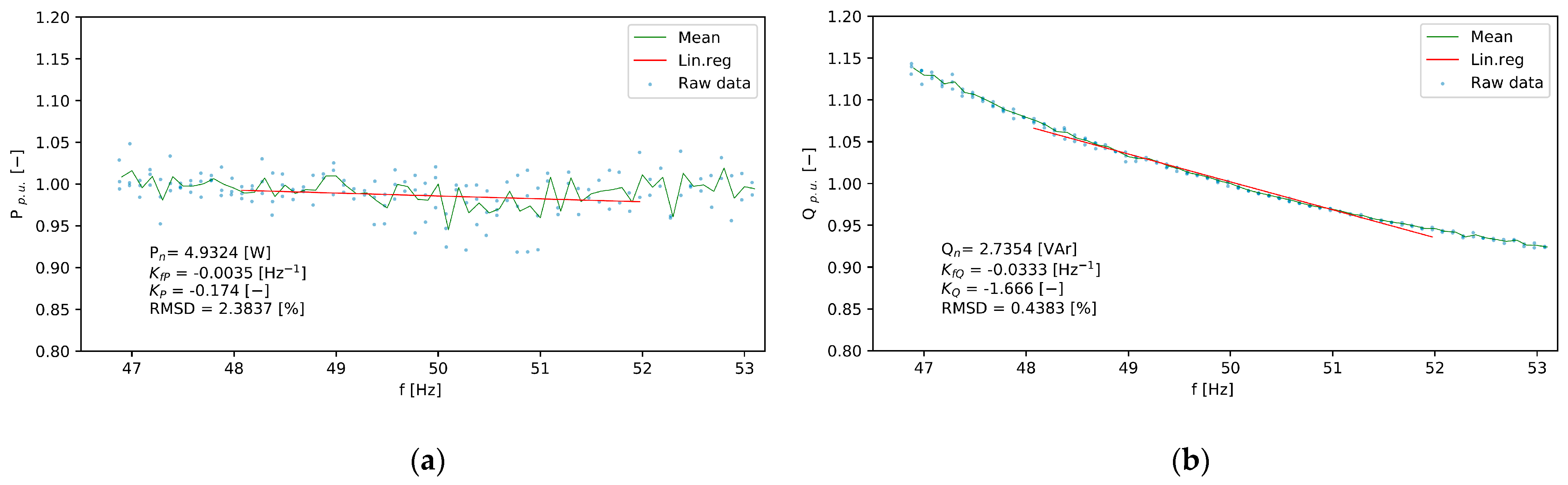
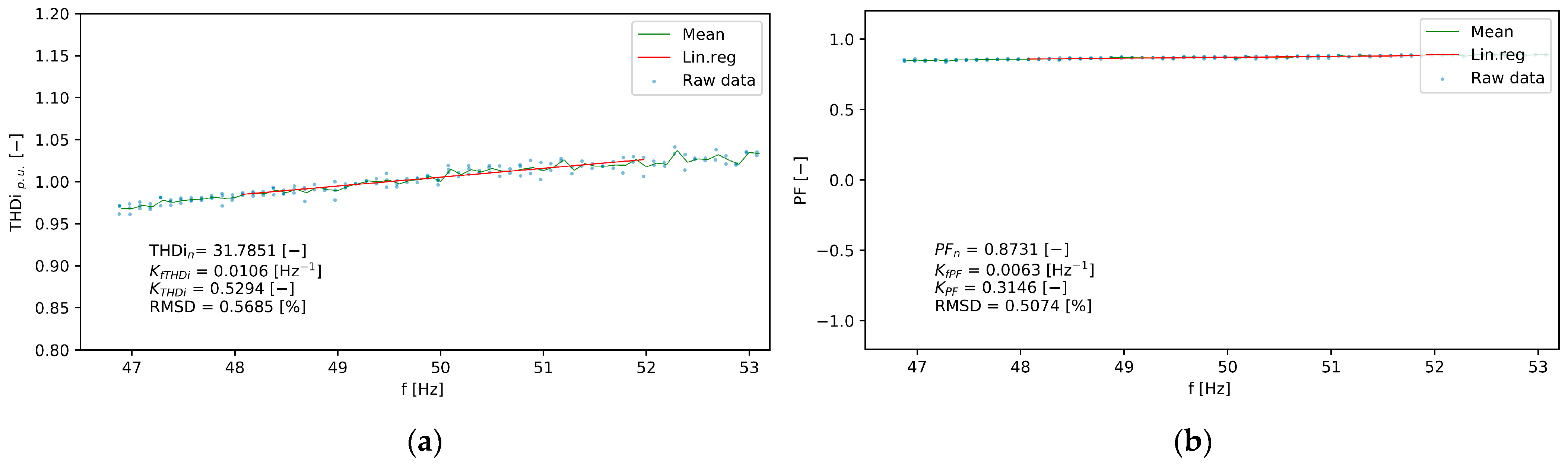
| Wi-Fi Router | 4.93 | −0.17 | 2.38 | 31.79 | 0.53 | 0.57 | Neg |
| LCD Monitor 17” | 25.42 | −0.04 | 0.81 | 88.97 | 0.00 | 0.15 | Neg |
| CRT Television 28” | 53.81 | 0.04 | 0.80 | 88.00 | −0.01 | 0.11 | Pos |
| Video Projector | 268.95 | 0.00 | 0.11 | 7.46 | −1.03 | 1.40 | no |
| Small Speakers | 1.43 | 0.01 | 1.43 | 95.71 | −0.01 | 0.06 | no |
| Microwave—stand by | 2.06 | −2.61 | 0.93 | 46.57 | −0.97 | 0.19 | Neg |
| Incandescent Lamp | 25.54 | −0.01 | 0.09 | 1.12 | −0.93 | 0.50 | no |
| Microwave | 1174.22 | 1.02 | 0.26 | 22.29 | −3.91 | 0.65 | Pos |
| Heat Gun | 955.45 | −0.02 | 0.14 | 0.57 | 0.20 | 3.15 | Neg |
| Vacuum Cleaner | 767.39 | −0.04 | 0.74 | 5.95 | 0.05 | 0.91 | Neg |
| Refrigerator | 113.03 | 0.41 | 0.41 | 9.43 | 0.22 | 0.36 | Pos |
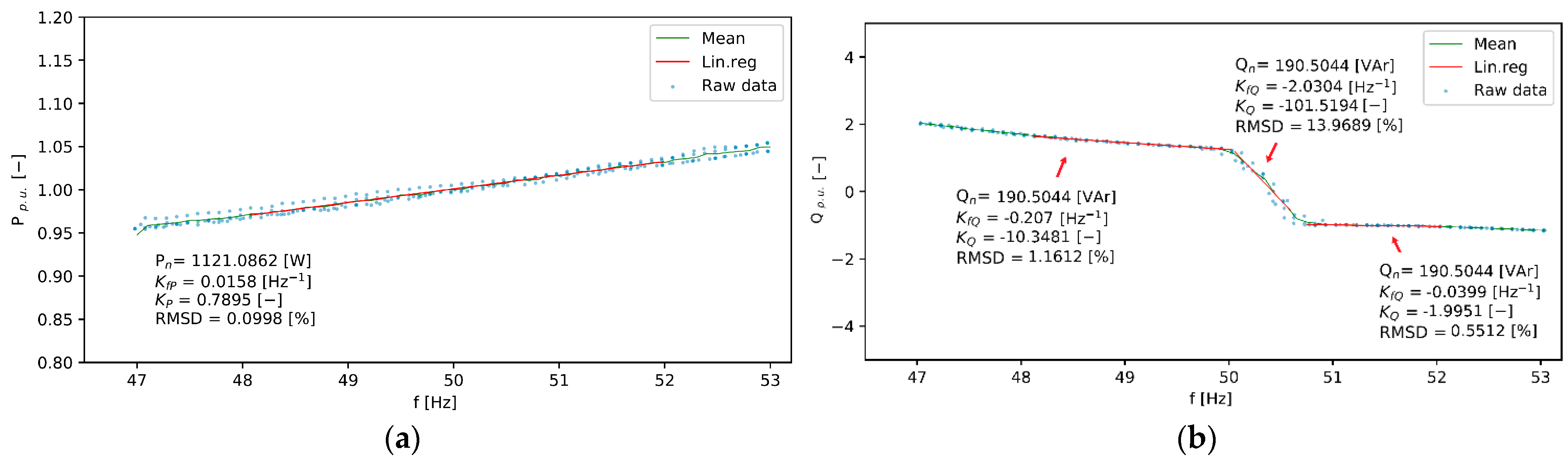
| Air Conditioner | 1121.09 | 0.79 | 0.10 | 17.18 | −3.69 | 0.59 | Pos |
| Rod Mixer A | 5.96 | −1.05 | 1.91 | 95.30 | 0.09 | 0.16 | Neg |
| Rod Mixer B | 28.84 | −0.13 | 0.57 | 77.37 | −0.03 | 0.11 | Neg |
| Hair Dryer | 590.07 | 0.18 | 1.84 | 25.76 | −0.58 | 4.52 | Pos |
| Device | Measured Reactive Power [VAr] | KQ [-] | RMSD [%] | Measured PF [-] | KPF [-] | RMSD [%] |
|---|---|---|---|---|---|---|
| Linear Fluorescent Lamp | 16.55 | −10.72 | 3.33 | 0.94 | 1.10 | 0.45 |
| Hight Pressure Sodium Lamp A | 209.51 | −0.79 | 1.21 | 0.39 | −0.28 | 0.72 |
| Hight Pressure Sodium Lamp B | 74.64 | −5.90 | 5.07 | 0.82 | 1.05 | 1.69 |
| Compact fluorescent Lamp | −18.34 | 0.29 | 0.72 | 0.59 | −0.08 | 0.09 |
| LED Lamp A | −16.00 | 0.51 | 0.10 | 0.95 | −0.05 | 0.01 |
| LED Lamp B | −19.22 | 0.86 | 0.17 | 0.95 | −0.09 | 0.02 |
| Wi-Fi Router | 2.74 | −1.67 | 0.44 | 0.87 | 0.31 | 0.51 |
| LCD Monitor 17” | −53.16 | 0.02 | 0.44 | 0.43 | −0.02 | 0.29 |
| CRT Television 28” | −101.39 | −0.04 | 0.43 | 0.47 | 0.03 | 0.18 |
| Video Projector | −36.57 | −0.01 | 0.65 | 0.99 | 0.00 | 0.01 |
| Small Speakers | −4.76 | −0.12 | 0.88 | 0.29 | 0.03 | 0.18 |
| Microwave—stand by | 3.30 | −7.39 | 1.75 | 0.53 | 1.81 | 0.33 |
| Incandescent Lamp | −0.40 | −0.99 | 0.27 | 1.00 | 0.00 | 0.00 |
| Microwave | 334.43 | −8.12 | 2.53 | 0.96 | 0.67 | 0.30 |
| Heat Gun | −5.73 | 0.10 | 1.06 | 1.00 | 0.00 | 0.00 |
| Vacuum Cleaner | 108.24 | 0.74 | 0.81 | 0.99 | −0.01 | 0.02 |
| Refrigerator | 122.54 | −0.94 | 0.12 | 0.68 | 0.50 | 0.15 |
| Air Conditioner | 190.50 | −10.35 (47–50.2 Hz) −101.52 (50.2–51 Hz) −1.99 (50.5–51 Hz) | 1.16 (47–50.2 Hz) 13.97 (50.2–51 Hz) 0.55 (50.5–51 Hz) | 0.98 | 0.18 | 0.22 |
| Rod Mixer A | 20.74 | −0.38 | 1.35 | 0.28 | −0.17 | 0.17 |
| Rod Mixer B | 5.05 | −22.72 | 119.83 | 0.63 | 0.02 | 0.07 |
| Hair Dryer | −121.02 | 1.35 | 14.57 | 0.90 | 0.15 | 1.60 |
| Device | KP [-] | KQ[-] | KTHDi [-] | KPF [-] | Light Source Category |
|---|---|---|---|---|---|
| Linear Fluorescent Lamp | −1.29 | −10.72 | 0.09 | 1.10 | Light sources with magnetic ballast |
| High-Pressure Sodium Lamp A | −1.65 | −0.79 | −1.46 | −0.28 | |
| High-Pressure Sodium Lamp B | −1.96 | −5.90 | 0.00 | 1.05 | |
| Compact fluorescent Lamp | 0.08 | 0.29 | 0.17 | −0.08 | Light sources with electronic ballast |
| LED Lamp A | 0.00 | 0.51 | −0.10 | −0.05 | |
| LED Lamp B | 0.00 | 0.86 | 0.68 | −0.09 | |
| Incandescent Lamp | −0.01 | −0.99 | −0.93 | 0.00 | Resistive light sources |
| Device | KP [-] | KQ [-] | PF [-] | ||||||
|---|---|---|---|---|---|---|---|---|---|
| Incandescent lights | 0.00 | 0.00 | −0.01 | 0.00 | 0.00 | −0.99 | 1.00 | 1.00 | 1.00 |
| Television | 0.00 | 0.00 | 0.04 | −4.50 | −2.60 | −0.04 | 0.80 | - | 0.47 |
| Heat Gun | - | 0.00 | −0.02 | - | 0.00 | 0.10 | - | 1.00 | 1.00 |
| Refrigerator | 0.53 | 0.50 | 0.41 | −1.50 | −1.40 | −0.94 | 0.80 | 0.79 | 0.68 |
| Air Conditioner | 0.98 | 0.90 | 0.79 | −1.30 | −2.70 | −10.35 (47–50.2 Hz) −101.52 (50.2–51 Hz) −1.99 (50.5–51 Hz) | 0.90 | 0.97 | 0.98 |
| Device | KP [-] | KQ [-] | PF [-] |
|---|---|---|---|
| Microwave—stand by | −2.61 | −7.39 | 0.53 |
| Microwave | 1.02 | −8.12 | 0.96 |
| Device | K [W/Hz] | KP [-] | Δfmax [Hz] | Δf [Hz] | Reg. Effect |
|---|---|---|---|---|---|
| Linear Fluorescent Lamp | −1.126 | −1.290 | −0.425 | −0.267 | Neg |
| High-Pressure Sodium Lamp A | −2.885 | −1.650 | −0.436 | −0.272 | Neg |
| High-Pressure Sodium Lamp B | −4.209 | −1.960 | −0.446 | −0.277 | Neg |
| Wi-Fi Router | −0.017 | −0.170 | −0.395 | −0.252 | Neg |
| LCD Monitor 17” | −0.020 | −0.040 | −0.392 | −0.251 | Neg |
| Microwave—stand by | −0.107 | −2.610 | −0.467 | −0.288 | Neg |
| Heat Gun | −0.334 | −0.020 | −0.391 | −0.250 | Neg |
| Vacuum Cleaner | −0.610 | −0.040 | −0.392 | −0.251 | Neg |
| Rod Mixer A | −0.125 | −1.050 | −0.419 | −0.264 | Neg |
| Rod Mixer B | −0.076 | −0.130 | −0.394 | −0.252 | Neg |
| LED Lamp A | 0.001 | 0.000 | −0.391 | −0.250 | no |
| LED Lamp B | −0.002 | 0.000 | −0.391 | −0.250 | no |
| Video Projector | −0.003 | 0.000 | −0.391 | −0.250 | no |
| Small Speakers | 0.000 | 0.010 | −0.391 | −0.250 | no |
| Incandescent Lamp | −0.005 | −0.010 | −0.391 | −0.250 | no |
| Compact fluorescent Lamp | 0.022 | 0.080 | −0.389 | −0.249 | Pos |
| CRT Television 28” | 0.041 | 0.040 | −0.390 | −0.250 | Pos |
| Microwave | 23.920 | 1.020 | −0.367 | −0.238 | Pos |
| Refrigerator | 0.929 | 0.410 | −0.381 | −0.245 | Pos |
| Air Conditioner | 17.701 | 0.790 | −0.372 | −0.241 | Pos |
| Hair Dryer | 2.150 | 0.180 | −0.387 | −0.25 | Pos |
Publisher’s Note: MDPI stays neutral with regard to jurisdictional claims in published maps and institutional affiliations. |
© 2021 by the authors. Licensee MDPI, Basel, Switzerland. This article is an open access article distributed under the terms and conditions of the Creative Commons Attribution (CC BY) license (http://creativecommons.org/licenses/by/4.0/).
Share and Cite
Beláň, A.; Cintula, B.; Cenký, M.; Janiga, P.; Bendík, J.; Eleschová, Ž.; Šimurka, A. Measurement of Static Frequency Characteristics of Home Appliances in Smart Grid Systems. Energies 2021, 14, 1739. https://doi.org/10.3390/en14061739
Beláň A, Cintula B, Cenký M, Janiga P, Bendík J, Eleschová Ž, Šimurka A. Measurement of Static Frequency Characteristics of Home Appliances in Smart Grid Systems. Energies. 2021; 14(6):1739. https://doi.org/10.3390/en14061739
Chicago/Turabian StyleBeláň, Anton, Boris Cintula, Matej Cenký, Peter Janiga, Jozef Bendík, Žaneta Eleschová, and Adam Šimurka. 2021. "Measurement of Static Frequency Characteristics of Home Appliances in Smart Grid Systems" Energies 14, no. 6: 1739. https://doi.org/10.3390/en14061739
APA StyleBeláň, A., Cintula, B., Cenký, M., Janiga, P., Bendík, J., Eleschová, Ž., & Šimurka, A. (2021). Measurement of Static Frequency Characteristics of Home Appliances in Smart Grid Systems. Energies, 14(6), 1739. https://doi.org/10.3390/en14061739