Article

Real-Time Implementation of the Predictive-Based Control with Bacterial Foraging Optimization Technique for Power Management in Standalone Microgrid Application

1
Department of Electrical Engineering, École de Technologie Supérieure, Montréal, QC H3C 1K3, Canada
2
CR2Ie, Sept-Îles, QC G4R 5B7, Canada
*
Author to whom correspondence should be addressed.
Energies 2021, 14(6), 1723; https://doi.org/10.3390/en14061723
Submission received: 10 February 2021 / Revised: 9 March 2021 / Accepted: 16 March 2021 / Published: 19 March 2021
(This article belongs to the Special Issue Power Management of Microgrids)

Abstract

:
In this paper, the predictive-based control with bacterial foraging optimization technique for power management in a standalone microgrid is studied and implemented. The heuristic optimization method based on the social foraging behavior of Escherichia coli bacteria is employed to determine the power references from the non-renewable energy sources and loads of the proposed configuration, which consists of a fixed speed diesel generator and battery storage system (BES). The two-stage configuration is controlled to maintain the DC-link voltage constant, regulate the AC voltage and frequency, and improve the power quality, simultaneously. For these tasks, on the AC side, the obtained power references are used as input signals to the predictive-based control. With the help of the system parameters, the predictive-based control computes all possible states of the system on the next sampling time and compares them with the estimated power references obtained using the bacterial foraging optimization (BFO) technique to get the inverter current reference. For the DC side, the same concept based on the predictive approach is employed to control the DC-DC buck-boost converter by regulating the DC-link voltage using the forward Euler method to generate the discrete-time model to predict in real-time the BES current. The proposed control strategies are evaluated using simulation results obtained with Matlab/Simulink in presence of different types of loads, as well as experimental results obtained with a small-scale microgrid.

1. Introduction

Diesel generator (DG) is still used as the main energy source in many remote areas. Although, diesel is costly, pollutant, and inefficient at light loads [1]. Moreover, in presence of nonlinear loads, the DG lifetime is affected by the harmonic currents. On the other hand, isolated areas often have a large potential for renewable energy sources (RES) such as solar and wind. Generally, the integration of RES in these isolated microgrids allows to decrease the operation cost as well as increase the reliability and efficiency of the system [2,3]. The RES are stochastic, so battery energy system (BES) is suggested to compensate for their intermittent properties. BES is a DC source in nature, it needs a controlled power converter such as a DC-DC buck-boost converter to operate properly and to adapt its output voltage to the DC-link voltage for standalone microgrid application. Moreover, with the help of the controlled power converters, one controls the power flows and protects the storage element [4,5]. However, the integration of non-renewable energy sources (NRESs) and their power converters with the existing diesel generators makes standalone microgrid applications more complex. Therefore, accurate control strategies and power management techniques should be employed to always ensure secure and effective operation [6].
For microgrid application control, centralized and decentralized control are used [7]. Regrading, the centralized control, a central decision controller gathers information and decides the action for the hierarchical control. This control requires communication between the central controller and all system elements [8]. For the decentralized control, each element is independent and achieves the tasks locally using the local measurements. According to [9], a compromise can be made between these two types of control by using control levels that differ by their time frame, time response, and communication requirement. Generally, the hierarchical control consists of three levels: primary, secondary, and tertiary [9]. The primary control, or local control, is characterized by its fastest response time and it operates with a decentralized approach. The secondary level, referred to as the energy management system, aims to fulfill the economic objective of the microgrid, i.e., it controls different energy sources in presence of load and weather conditions variations as well as the state of charge of the BES. This level of control is characterized by its slower time response so that the secondary and the primary control are decoupled, they employ sample measurement data to reduce the communication link bandwidth. This can improve the control performance because it allows more time to perform complex calculations. The tertiary control level is considered as a part of the utility grid, it is not considered in this paper.
Several control strategies for the primary control level had been reported in the literature [10]. Among these control strategies, predictive-based control is proposed in [11]. This technique shows a fast dynamic response compared to the existing technique, and it can handle nonlinearities. This technique uses the measured system data and parameters to predict the future behavior of the system. These predictions are then evaluated by a cost function to reduce the error between the prediction and its reference. This concept is applied to achieve many tasks in many applications for grid-connected microgrid [11,12,13] and islanding microgrid [4,14], for power management [11,12], power quality [4,13,14], and synchronization [15]. However, predictive control also has drawbacks as reported in [16]. Some compromises need to be made when selecting the discretization method, between model accuracy and calculation complexity; but also, when selecting the sampling time, between better performance and computation time [16].
Generally in power management, the objective function may include high order polynomial function, so heuristic optimization methods are proposed to handle this issue [17,18,19]. Particle swarm optimization (PSO) is proposed in [17] and ant colony optimization (ACO) in [18]. Further in 2002, Passino proposed the bacterial foraging optimization (BFO) method, this technique emulates the behavior of E. coli bacteria [20]. This technique is proposed for different applications, including tuning proportional-integral (PI) controller parameters [21,22], power system reconfiguration and power loss minimization [23], or estimating PV parameters [24]. Furthermore, hybrid BFO/PSO methods are proposed for solar tracking [25] or multi-loop controller design [26]. The BFO technique is compared to other optimization techniques in the literature and it shows better performance under severe conditions for many applications. In [27], the performance BFO method is compared to an enhanced non-dominated storing genetic algorithm (NSGA-II) and multi-objective PSO (MOPSO) for a multi-objective problem. The obtained results show that the multi-objective BFO is robust, stable, and precise compared to other techniques. According to [28], the efficiency of the genetic algorithm (GA) is affected by the premature convergence but the BFO method possesses a much higher possibility to override the local minima. Moreover, the performance of GA and BFO are compared for automatic generation control to optimize parameters. The obtained results show that the BFO method performs well with faster results due to the smaller number of iterations. In [29], authors have compared the BFO method with GA, PSO, GA/PSO, and simulated annealing (SA) methods to find the optimal location and size of several DGs in a 33 bus and 69 bus test systems, to minimize the losses and operational costs, and to improve the voltage stability in the distribution system in presence of different types of loads. Compared to other optimization methods, the BFO method presents accuracy and precision to find the optimum solutions. In [30], the heuristic optimization methods as, GA, binary particle swarm optimization (BPSO), BFO, wind-driven optimization (WDO), and the proposed hybrid genetic wind-driven (GWD) algorithm are compared to the BFO technique for power management in a smart grid application. Many features as scheduling residential loads between peak hours and off-peak hours while maximizing user comfort, minimizing the electricity cost, and the peak to the average ratio for a single home, and later for multiple homes are evaluated. The obtained results show that the GWD method performs well in reducing the electricity costs, and the GA method provides an optimal global solution and gives a better convergence rate. Regarding, the small population groups, BPSO and BFO converge faster but BFO shows the smallest computational burden. In [31], the BFO and PSO methods are compared for a real-time calculation of active and reactive power references, both methods show accurate results however, the BFO method possess less calculation steps.
In this paper, the implementation of a two-level control strategy based on the BFO method and the predictive control in a standalone microgrid is proposed. The BFO technique is employed to determine the power references from the load and NRESs power. The two-level control strategy is designed to maintain constant the DC-link voltage, regulate the voltage and frequency at the point of common coupling (PCC) and improve the power quality simultaneously. For the AC side, the obtained power references are used as input to the predictive control so that it can control the power exchanges while regulating the PCC voltage and frequency but also improve the power quality. Regarding the DC side, predictive control is used for the DC-link voltage regulation.
The proposed standalone microgrid configuration is presented in Section 2. The predictive and BFO controllers are detailed in Section 3. Simulation and experimental results as well as a discussion are given in Section 4. Finally, the presented work is concluded in Section 5.

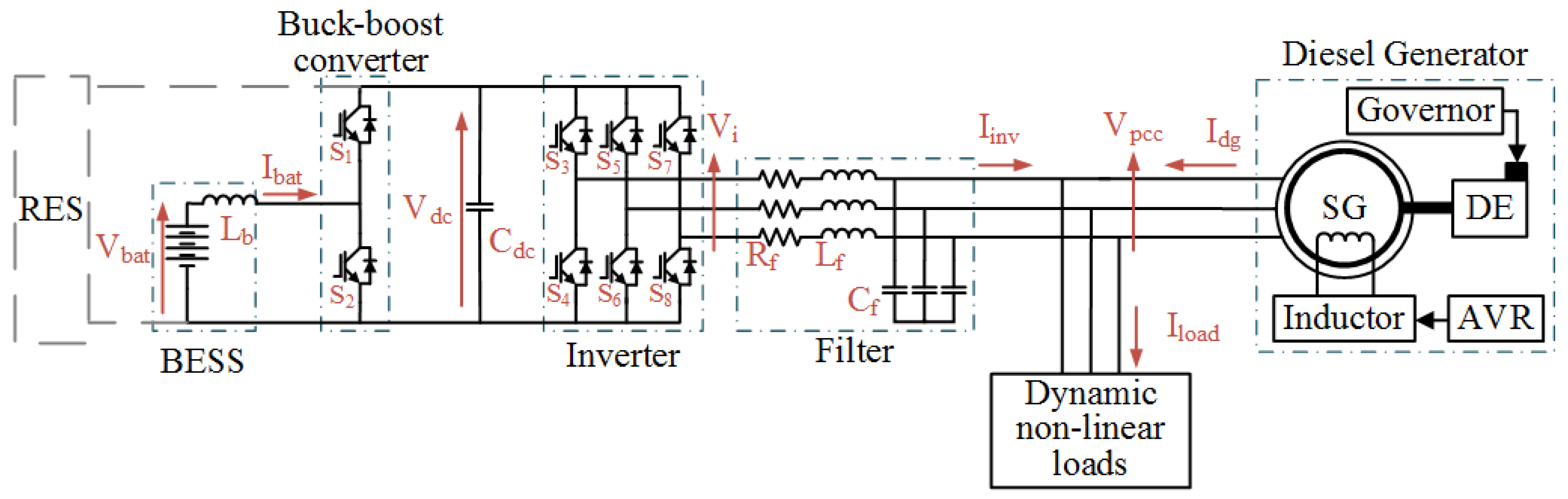
2. Microgrid Description

The proposed microgrid configuration is shown in Figure 1. It consists of Diesel Engine (DE) coupled with a Synchronous Generator (SG), forming a DG that is connected directly to the PCC. A BES is connected to the DC-link through a DC-DC buck-boost converter. An inverter and a RLC filter are used between the AC and the DC sides of the standalone microgrid. Both converters are controlled with predictive control. The DC-DC buck-boost converter is responsible for the DC-link voltage regulation by controlling the BES current, and the inverter is responsible for the PCC voltage and frequency regulation, power quality but also power management. For these tasks, the BFO and predictive control are employed. RES is not considered in this study but could be connected to the DC-link. Finally, the standalone microgrid supplies dynamic linear and non-linear loads.

3. Control Strategies

This section details the different control strategies for the two-level-based configuration. For the inverter side, the predictive-based control, which is used to predict the inverter current, and BFO, which is used to estimate the inverter reference current, are detailed. In addition, in this section, the predictive-based control for the DC-DC buck-boost converter used to estimate the BES current to regulate the DC-link voltage is given in detail.
Figure 2 shows the relation between the BFO technique and predictive-based control for the inverter. As one can see, the BFO technique uses measured power data (Pload, Pinv, Qload, Qdg, Qinv) and a rated value (Pdg,rated) to estimate the active and reactive power references (Pref and Qref) that are used by the predictive control algorithm as input signals to estimate the inverter current reference.

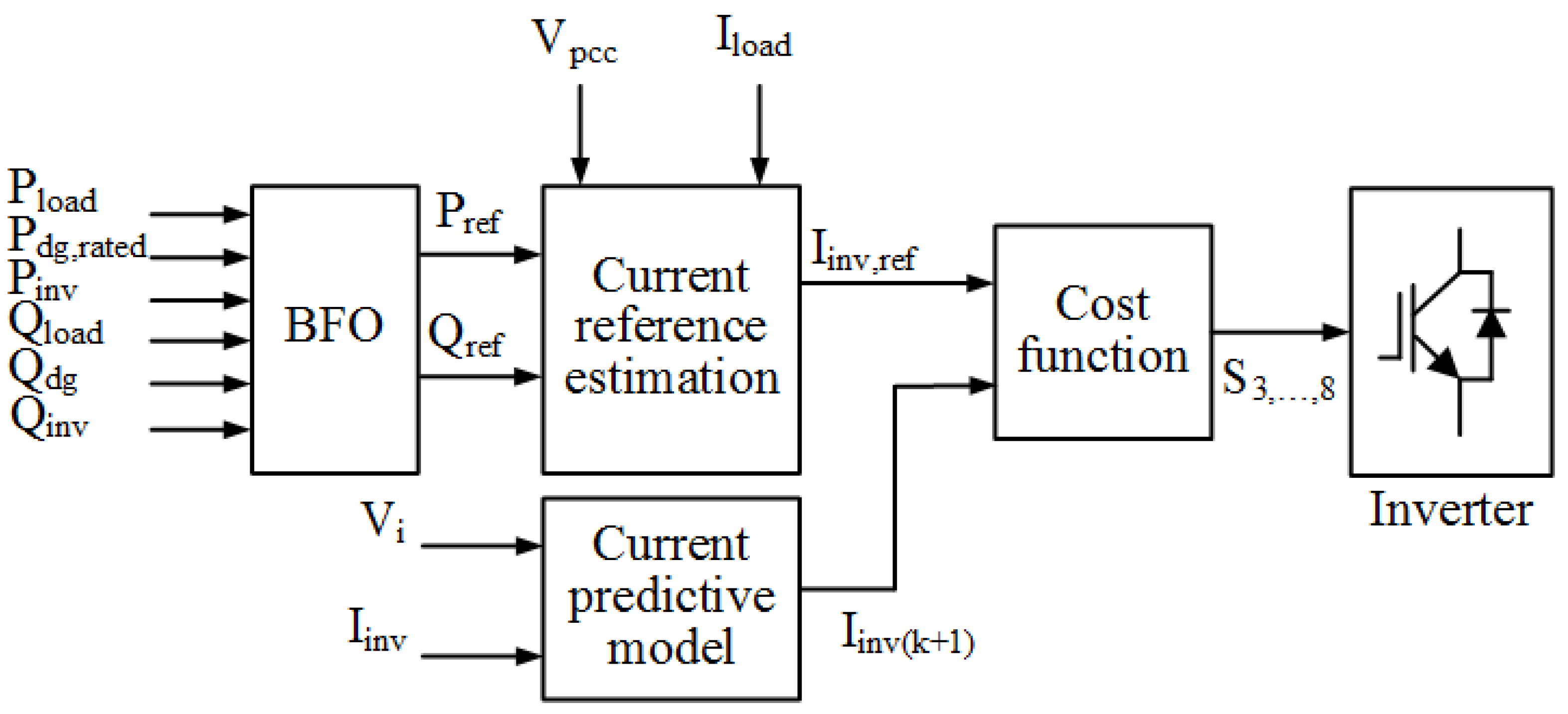
3.1. Inverter Predictive Control

As shown in Figure 2, the predictive-based control is made of three steps: (1) reference current estimation, (2) current predictive model, and (3) a cost function.

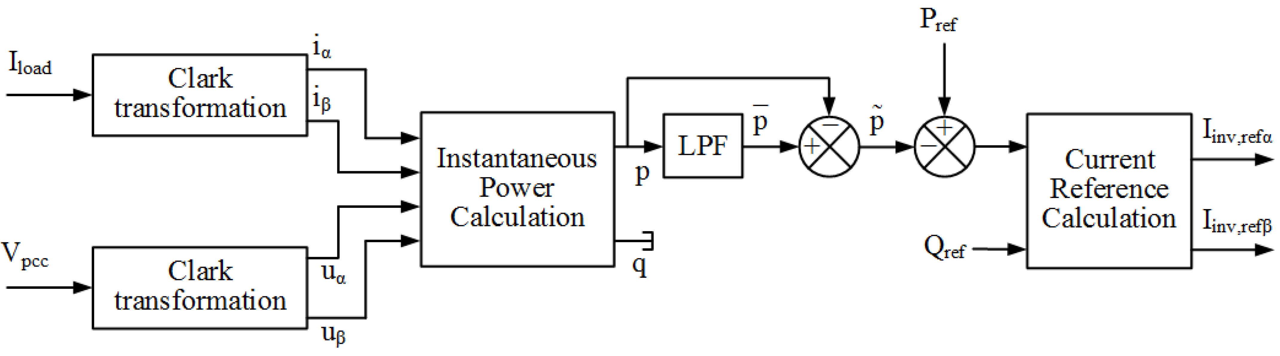
3.1.1. Inverter Reference Current Estimation

The current reference is needed to ensure the power management, as well as the power quality and voltage and frequency regulation at the PCC. For power management, the output signals of the optimization technique are used, as shown in Figure 2 and Figure 3. For the power quality, the measured load current (Iload) and PCC voltage (Vpcc) are transformed into complex quantities using the Clark transformation (1). Then, the instantaneous active and reactive power are computed using (2). The active power is obtained based on an average ( p ¯ ) and an oscillating component ( p ˜ ) which contains the harmonics. The low pass filter is used to keep only the oscillating component, which is then substracted to the new active power reference (Pref) obtained using the BFO technique. Regarding, the reactive power reference, (Qref) is used simply to compute the new current references (Iinv,refα and Iinv,refβ) as demonstrated in Figure 3 and expressed in (3).
The Clark transformation is employed because it allows to simplify the analysis of three-phase quantities, the system is transformed from a two rotating axes reference frame into a two stationary axes reference frame, without estimating the phase angle at the PCC using the conventional phased locked loop (PLL). Therefore, three dimensions problems are transformed into two dimensions problems.
[   u α u β   ] = 2 3 [ 1 1 2 1 2 0 3 2 3 2 ] [ V pcca V pccb V pccc ] [   i α i β   ] = 2 3 [ 1 1 2 1 2 0 3 2 3 2 ] [ I loada I loadb I loadc ]
  [ p q ] = [ u α u β u β u α ] [ i α i β ]
  [ I inv , ref α I inv , ref β ] = 1 u α 2 + u β 2 [ u α u β u β u α ] [ P ref p ˜ Q ref ]

3.1.2. Current Predictive Model

In this step, a vector with the possible values of the inverter current on the next sampling time is computed. First, the vector of the possible inverter output voltage is needed, it is obtained based on the behavior of the inverter switches as expressed in (4). With the help of Kirchhoff’s laws, one obtains the mathematical model of the PCC voltage (5). To implement a digital controller, the PCC voltage as expressed in (5) is transformed into a discrete-time equation using Euler forward method which is detailed in (6). Based on (5), and (6), one obtains the vector of the inverter output current possible values on the next sampling time (IINV(k+1)) as expressed in (7).
  V i = { 2 3 V dc e j ( i 1 ) π 3 ; i = 1 , 2 , , 6 0 ; i = 0 , 7
  V pcc = V i L f dI inv dt R f I inv
dx dt = x ( k + 1 ) x ( k ) T s
  I inv ( k + 1 ) = T s L f V i T s L f V pcc ( k ) + I inv ( k ) ( 1 R f T s L f )

3.1.3. Cost Function

To select the prediction, which is closer to the reference, the cost function (8) is employed. It uses the square error of the active and reactive parts of the reference and the predictions. For each prediction, the cost function is computed and the prediction with the smallest cost is the closest to the reference. Due to the calculation of the predictions using the inverter output voltage and the switches behavior, one knows the switches profile which corresponds to each prediction. Therefore, from the cost function values, one can deduce the switch’s profile to apply to the inverter so that on the next sampling time the inverter current follows the reference.
g 1   = ( I inv , ref α I inv ( k + 1 ) α ) 2 + ( I inv , ref β I inv ( k + 1 ) β ) 2

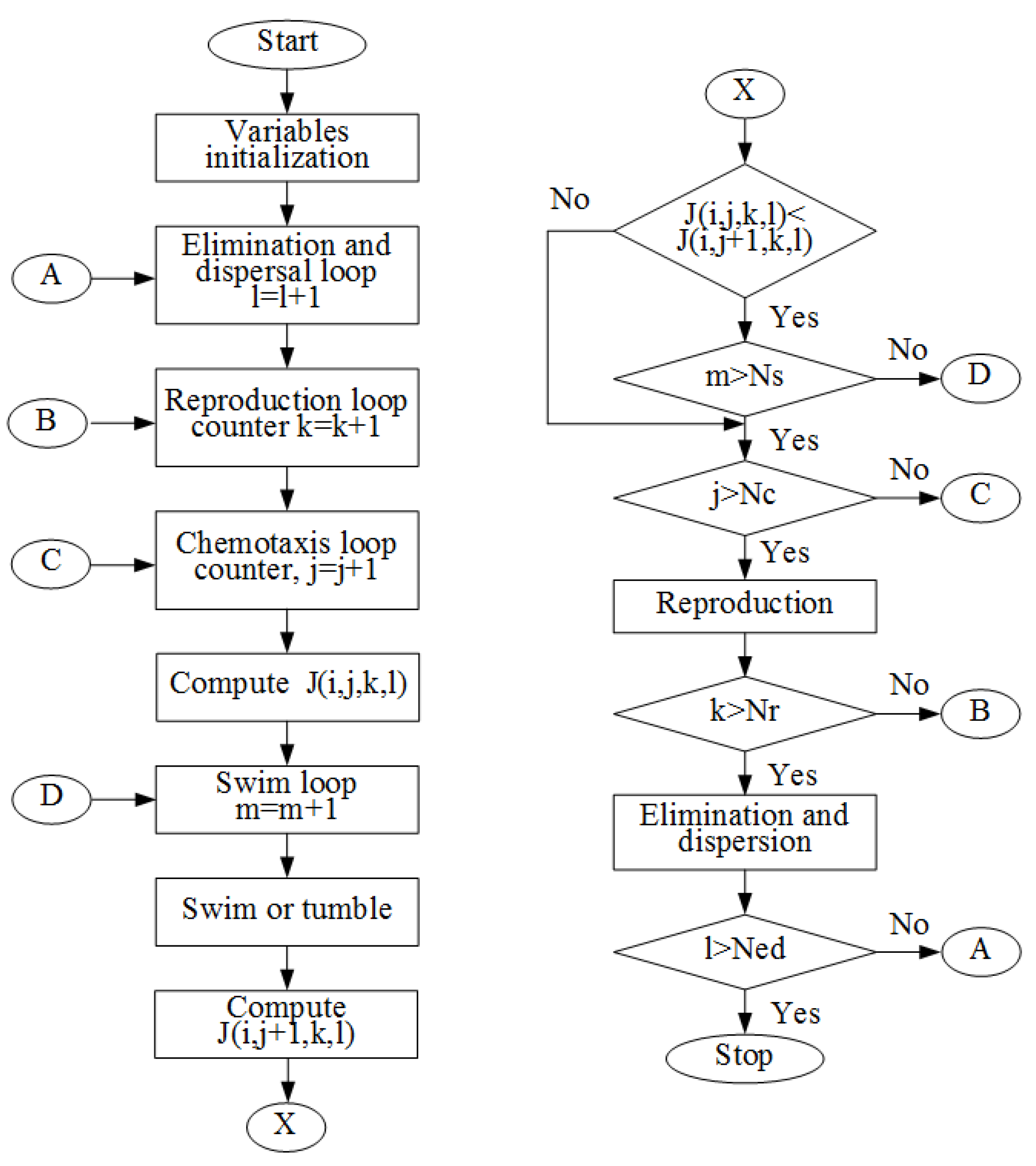
3.2. Bacterial Foraging Optimization Technique

The BFO technique is employed to calculate the active and reactive power references using the powers of the NRESs as shown in Figure 2. It consists of five steps as (1) initialization, (2) chemotaxis, (3) swarming, (4) reproduction, and (5) elimination and dispersal. The following subsections give more details about these steps. The flowchart given in Figure 4 shows the steps of the BFO technique.

3.2.1. Initialization

For the initialization, many parameters such as the number of bacteria (S), number of chemotaxis steps (Nc), number of swim steps (Ns), number of reproductive steps (Nr), and number of elimination and dispersal steps (Ned), should be defined. Unfortunately, there is no mathematical approach to define the optimal value of these parameters, for this reason, a heuristic method is employed, and the values of these parameters are given in Table A1. The initial positions of the bacteria are defined randomly around the measured powers. The reference vector θr is defined as detailed in (9). As already indicated, the main task of the proposed BFO technique is to estimate the power references. For this application, the objective is to operate the DG at its rated power, the DG should deliver the same amount of active power all the time. Furthermore, the reactive power should be supplied by the inverter. In addition, the frequency of activation of the BFO technique should be defined. To make sure that the objectives will be accomplished, the new power references should be computed often. Seeing that the developed BFO controller consists of many interconnected control loops, the computation time is important. A compromise needs to be made here and to ensure a soft transition. For the optimal operation of the BFO technique, the new power references are computed every 5 ms.
  θ r = ( θ rP = P load P dg , rated θ rQ = Q load Q dg )
where Pload, Qload, Pdg,rated and Qdg represent the measured active and reactive power at the load, the active rated power of the DG, and the measured reactive power at the DG, respectively.

3.2.2. Chemotaxis

Regarding the chemotaxis step, the bacteria’s movement is emulated. When a bacterium keeps moving in the same direction, it is called swimming and when it changes direction, it is called tumbling. Equation (10) describes these phenomena.
  θ ( i , j + 1 , k , l ) = θ ( i , j , k , l ) + c × sgn ( Δ )
where θ(i,j,k,l) represents the ith bacteria, at the jth chemotaxis step, at kth reproduction step, and lth elimination and dispersal step. Then, θ(i,j + 1,k,l) represents the same bacteria at the next chemotaxis step. The parameters c and Δ respectively represent the length and the direction of the movement. They are generated randomly.
A cost function is used to evaluate how each bacterium is close to the reference. As expressed in (11), the cost function is defined as the absolute value of the difference between a bacterium position and the reference position.
  J ( i , j , k , l ) = abs ( θ r θ ( i , j , k , l ) )

3.2.3. Swarming

E. coli bacteria can communicate about their current position whether it is a good or a bad direction to converge. To emulate this swarming phenomenon, the cost function needs to be modified as detailed in (12) and (13).
  J CC ( θ , θ i ) = i = 1 S J CC i ( θ , θ i ) = i = 1 S [ d a e ( w a m = 1 p ( θ θ i ) 2 ) ] + i = 1 S [ h r e ( w r m = 1 p ( θ θ i ) 2 ) ]
  J ( i , j , k , l ) = J ( i , j , k , l ) + J CC ( θ , θ i )
where da, wa, hr, and wr represent the depth and width of the attractant signal, the height, and width of the repellant effect, respectively. In (12) the notations are simplified, θ represents the bacterium understudy, and θi represents the bacteria that already moved.

3.2.4. Reproduction

Once all the bacteria have moved and computed their new cost function, a classification is made based on their cost function value. Then, the half with the higher cost function values dies while the other half splits in two, at the same position. So that the number of bacteria is constant, and the population is healthier.

3.2.5. Elimination and Dispersal

E. coli bacteria sometimes die or get dispersed in the environment without any reason. In our application, this phenomenon helps the chemotactic process because it reduces the chances to be trapped in a premature local solution. A probability coefficient (Ped) is defined, and each bacterium is subjected to elimination and dispersal with this probability. When a bacterium is eliminated it is replaced with a new one with a random position to keep constant the population.

3.3. DC-DC Buck-Boost Converter Predictive Control

The predictive-based control is also employed to control the DC-DC buck-boost converter. The three same steps are needed as, (1) the current predictive model, (2) the current reference estimation, and (3) a cost function as demonstrated in Figure 5.

3.3.1. Current Predictive Model

Using Kirchhoff’s laws, the mathematical model of the DC-DC buck-boost converter is developed. Equation (14) is obtained when S1 is closed and S2 is open and, Equation (15) is obtained when S1 and S2 are respectively open and closed. As the voltage regulation is achieved by controlling the BES current, only the current equations are needed. Again, the forward Euler method (6) is used to convert the system into a discrete-time model. Finally, the predictions (16) are obtained as
dI bat dt = 1 L b V bat 1 L b V dc
dI bat dt = 1 L b V bat
  { I bat ( k + 1 ) 1 = T s L b V bat ( k ) T s L b V dc ( k ) + I bat ( k ) I bat ( k + 1 ) 2 = T s L b V bat ( k ) + I bat ( k )

3.3.2. BES Reference Current Estimation

As the DC-DC buck-boost controller aims to regulate the DC-link voltage by controlling the BES current, two components need to be considered. (1) The amount of current coming from the AC side of the microgrid, which is computed using the active power of the inverter and the DC voltage reference; and (2) the amount of current needed to regulate the voltage, which is calculated using the error between the DC-link voltage and its reference. Finally, this value represents the amount of current going through the inverter and it needs to be adjusted to represent the amount of current the BES needs to store.
  I bat , ref = V dc , ref V bat [ P inv V dc , ref + C dc T s ( V dc , ref V dc ) ]

3.3.3. Cost Function
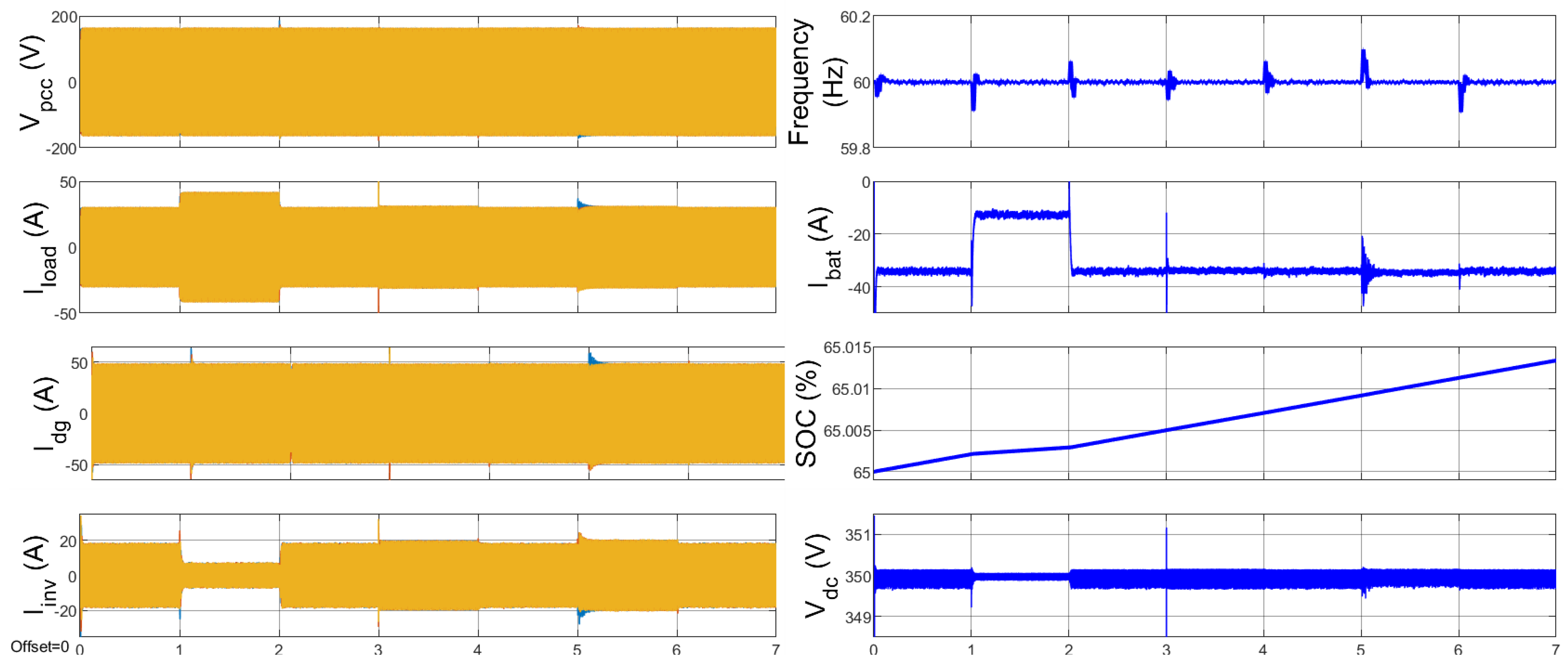
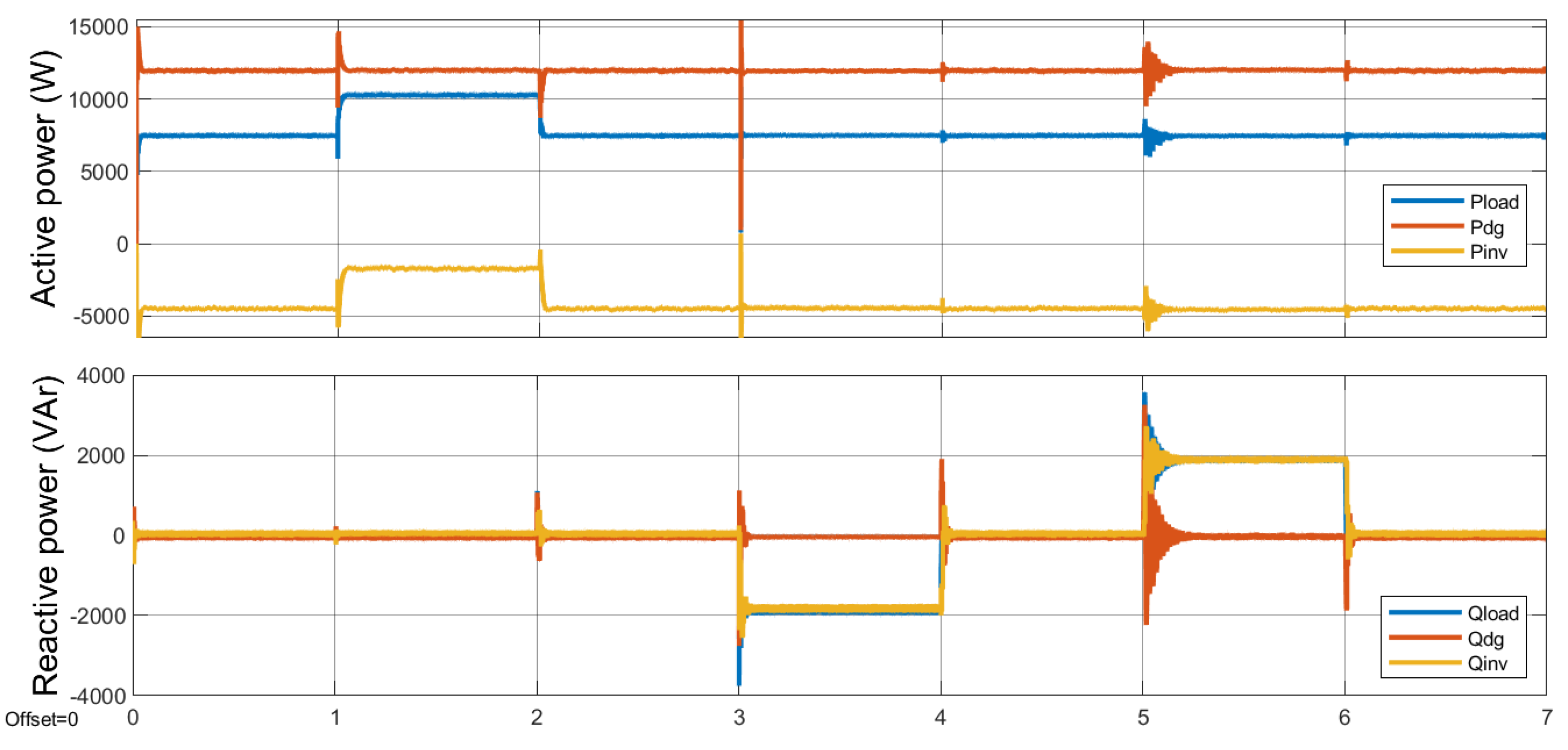
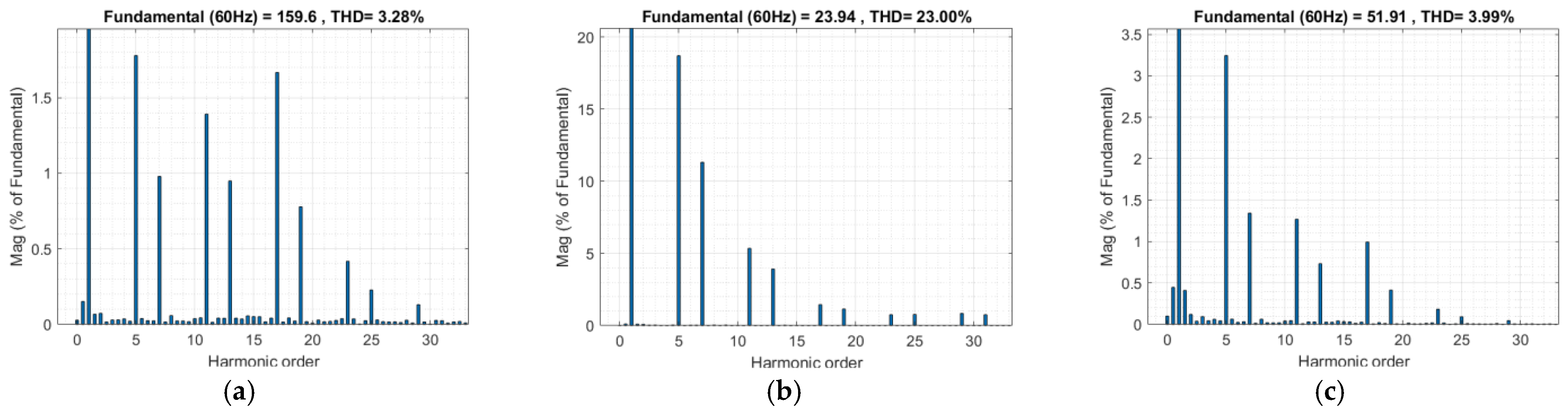
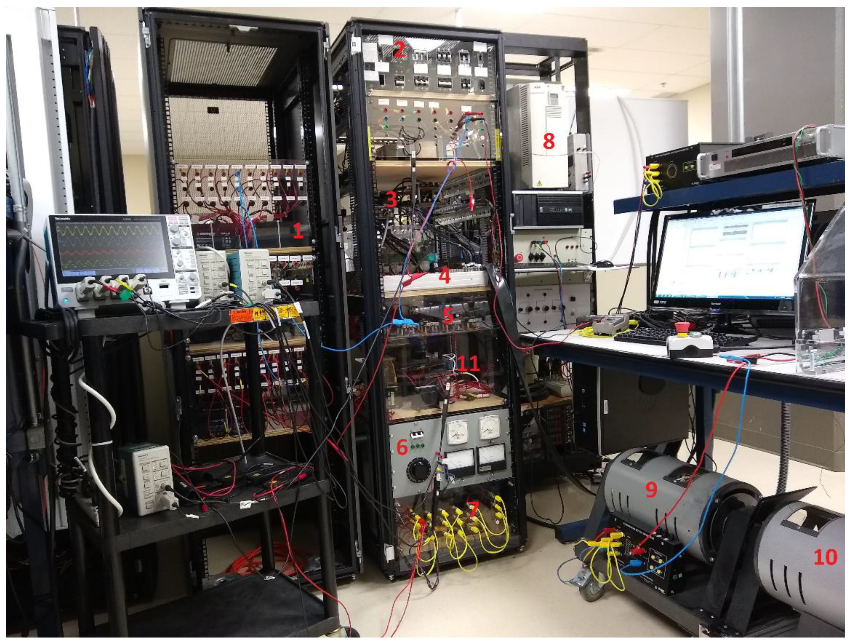
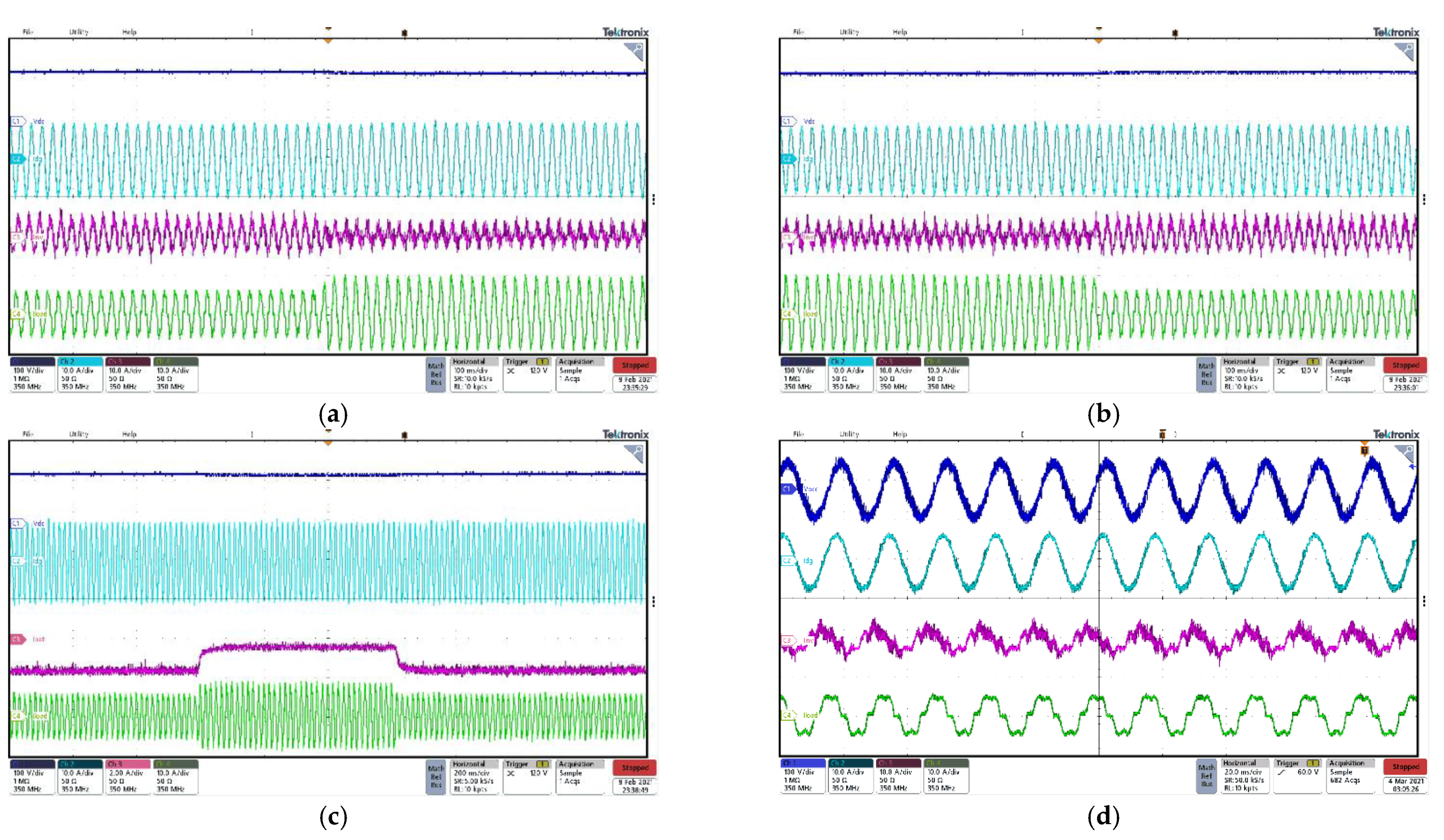
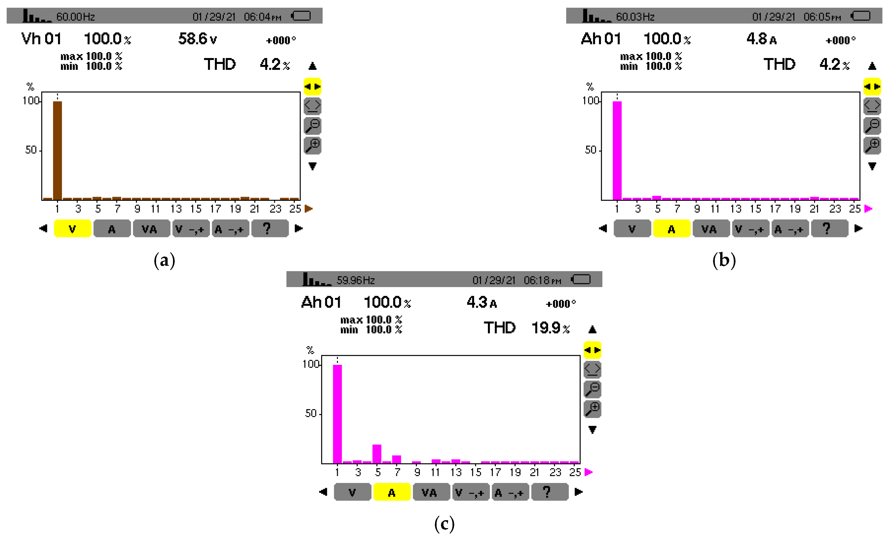
The cost function (18) is employed to evaluate which of the two predictions is closer to the reference. It uses the absolute value of the error between the reference and the prediction as presented in (18). The prediction with the smaller cost function is closer to the reference. Therefore, if Ibat(k + 1)1 possesses the smallest cost function value, S1 is closed and S2 open on the next sampling time and if Ibat(k + 1)2 possesses the smallest cost function, S1 is open and S2 is closed.
g 2 = | I bat , ref I bat ( k + 1 ) 1 , 2 |

4. Results

To validate the proposed control strategies for the DC-DC buck-boost converter and three-phase inverter, simulation and experimental tests are realized in presence of a different types of loads. The simulation tests are performed using Matlab/Simulink. Figure 6 shows the PCC voltage (Vpcc), the load current (Iload), the DG current (Idg), the inverter current (Iinv), the frequency of the system, the BES current (Ibat), the state of charge of the BES (SOC), and the voltage of the DC-link (Vdc). In Figure 7, the active and reactive power of the load (Pload and Qload), the DG (Pdg and Qdg), and the inverter (Pinv and Qinv) are demonstrated. Then, in Figure 8, the power references generated using BFO estimation technique (Pref and Qref) and the active and reactive power of the inverter (Pinv and Qinv), are presented. It is observed that three different loads are connected at the system at different times as (1) a constant 8 kW resistive load and from t = 1 s to t = 2 s additional resistive load of 3 kW, (2) from t = 3 s to t = 4 s a 2 kVAr capacitive load is connected, and (3) from t = 5 s to t = 6 s an inductive load of 2 kVAr is connected. One sees clearly in Figure 6 that the PCC voltage, the frequency of the system as well as the DC-link voltage are well regulated during the transitions. One sees that the overshoot and undershoot in DC-link voltage is minimized, which confirms the developed predictive-based controller. In addition, the DG current is kept constant during all times, but the inverter current varies with the variation of loads, which confirms that the balance in power is ensured by the BES for our application. One observes that BES current from t = 1 s to t = 2 s is increased but for the rest of the simulation is kept constant and is with a negative sign, which means that BES is charging. In Figure 7, the same phenomena are shown, the active power generated from the DG is constant and the inverter active power varies with the variation of load power demand. Regarding, the reactive power, one can see that the DG reactive power is almost zero and the inverter reactive power varies with the variation of load reactive power demand. In Figure 8, the performance of the inverter power references is presented, one observes that the estimated active and reactive power using predictive based control follows their references generated using the BFO optimization technique, which confirms the good operation of both techniques used to control the two-level three-phase inverter to supply the load with constant voltage and frequency and mitigate the harmonics.
Figure 9 shows the waveform of the PCC voltage (Vpcc), the load current (Iload), the DG current (Idg) and the inverter current (Iinv) in presence of a non-linear load. One can see that the waveforms of the PCC voltage and DG current are balanced and sinusoidal. In this case, the inverter acts as an active shunt filter, it compensates harmonics created by the nonlinear loads and balance the DG currents. One sees in Figure 10 that the total harmonic distortion (THD) of the PCC voltage is 3.28% and the THD of the DG current is 3.99% and that the THD of the load current is 23%. Therefore, the PCC voltage and DG current are below the limit of 5% and respects IEEE Std 519-1992, IEEE recommended practices and requirement for harmonic control in the electrical power system.
Figure 11 demonstrates the hardware prototype used to validate the performance of the developed control strategies for the two-power converter. It consists of (1) lead acid batteries, (2) loads, (3) three-phase inverter, (4) dSPACE, (5) voltage and current sensors, (6) auto-transformer, (7) RLC filter, (8) ABB drive, (9) SG, (10) Induction Machine, and (11) DC-DC Buck-boost converter.
Experimental results of the DC-link voltage (Vdc), DG current (Idg), inverter current (Iinv), and load current (Iload) are presented in Figure 12a,b. Figure 12c shows the DC-link voltage (Vdc), DG current (Idg), BES current (Ibat), and load current (Iload). Figure 12d shows the PCC voltage (Vpcc), DG current (Idg), inverter current (Iinv), and load current (Iload). It is observed in Figure 12a,b, that the load increases and decreases, respectively, at t = 0.5 ms, but the DG current stays constant and the inverter current varies with the variation of the load, it decreases and increases with increasing and decreasing of loads. One can see in Figure 12c that the load is increased at t = 0.6 s and decreased at t = 1.2 s, the DG current stays constant and the BES current is increased and decreased with the load variations. The BES current is of the negative sign which means that the battery is being charged by the DG. Indeed, the balance of power in the system is ensured by the BES. One observes that DC-link voltage varies slightly, which confirms the robustness of the developed predictive-based control for the DC-DC buck-boost converter. From Figure 12d, one observes that the inverter acts as an active filter, it compensates the harmonics current created by the non-linear load and balance the DG current and PCC voltage, these results can be compared to the simulation results presented in Figure 9. In Figure 13, the harmonic spectrum of the PCC voltage, load current, and DG current are presented. One sees that THD of the PCC voltage (a) and DG current (b), are less than 5%, which respects the IEEE-Std 519-1992. This confirms that the predictive-based control operates well under the presence of nonlinear loads.

5. Conclusions

In this paper, the implementation of predictive-based control with the BFO technique for a standalone microgrid has been investigated. The two-level configuration is controlled to regulate the DC-link voltage, the voltage, and the frequency, and to improve the power quality at the PCC. For the AC side, the power references obtained with the BFO method are used as inputs to the predictive control so that it can control the power exchanges while regulating the PCC voltage and frequency but also improve the power quality. For the DC side, the predictive control is used to regulate the DC-link voltage by controlling the DC-DC buck-boost converter. The obtained simulation and experimental results are satisfactory under the presence of all conditions. The power quality, voltage, frequency, and power exchanges are achieved without any overshoot nor undershoot of the DC-link voltage. The DG is kept always operating at its rated power and the reactive power is supplied by the BES, which confirms the robustness, accuracy, and precision of the developed BFO technique-based for standalone microgrid application. The integration of other energy sources such as RES should be considered in future studies which would modify the objectives of the microgrid. The BFO algorithm should be modified to include theses new objectives and to make the power management more efficient.

Author Contributions

This paper was a collaborative work between the four authors. F.D. contributed to the design of the proposed control strategies, simulation, and experimental results, and drafted the manuscript. M.R. performed in the design of system elements, experiments, and revision of the manuscript. H.I. and A.C. supervised the work, provided advice on methodology and results. All authors have read and agreed to the published version of the manuscript.

Funding

This work is supported by RQEI (Réseau québécois sur l’énergie intelligente).

Institutional Review Board Statement

Not applicable.

Informed Consent Statement

Not applicable.

Data Availability Statement

Not applicable.

Acknowledgments

Validation in real-time had been realized at École de Technologie Supérieure in the laboratory of Power Electronics and Industrial Control Research Group (GREPCI), in Montreal, Quebec, Canada.

Conflicts of Interest

The authors declare no conflict of interest.

Appendix A

Table A1. Parameters of the System.
ElementsParameters
Synchronous GeneratorSn = 12 kVA, Vn = 208 V, fs = 60 Hz, 2 P = 4, Rinternal impedance = 0.8160 Ω, Linternal impedance = 0.8104 × 10⁻³ H, J = 3.895 × 10⁶ kg.m2
BESVn = 120 V, Rated capacity: 400 Ah, Vcut-off = 90 V, VFully-charge = 137.3 V,
Idischarge-nom = 8 A, rinternal =0.0625 Ω, Lbat = 0.25 mH
LoadsPconstant = 8 kW, Pdynamic = 3 kW, QdynamicC = 2 kVAr, QdynamicL = 2 kVAr
Rsnl = 1 Ω, Lsnl = 0.5 ×10⁻³ H, Rnl = 10 Ω, Lnl = 10 × 10−3 H
Filter Lf = 8.5 × 10⁻³ H, Cf = 40 × 10−6 F, Rf = 0.2 Ω
BFOS = 20; Nc = 8; Ns = 12; Nre= 4; Ned= 2; Ped = 0.3

References

  1. Rezkallah, M.; Singh, S.; Singh, B.; Chandra, A.; Ibrahim, H.; Ghandour, M. Implementation of Two-Level Coordinated Control for Seamless Transfer in Standalone Microgrid. IEEE Trans. Ind. Appl. 2021, 57, 1057–1068. [Google Scholar] [CrossRef]
  2. Dubuisson, F.; Rezkallah, M.; Chandra, A.; Saad, M.; Tremblay, M.; Ibrahim, H. Control of Hybrid Wind–Diesel Standalone Microgrid for Water Treatment System Application. IEEE Trans. Ind. Appl. 2019, 55, 6499–6507. [Google Scholar] [CrossRef]
  3. Sidorov, D.; Panasetsky, D.; Tomin, N.; Karamov, D.; Zhukov, A.; Muftahov, I.; Dreglea, A.; Liu, F.; Li, Y. Toward Zero-Emission Hybrid AC/DC Power Systems with Renewable Energy Sources and Storages: A Case Study from Lake Baikal Region. Energies 2020, 13, 1226. [Google Scholar] [CrossRef] [Green Version]
  4. Dubuisson, F.; Chandra, A.; Rezkallah, M.; Ibrahim, H.; Singh, B. Predictive Based Control Algorithm for Hybrid Diesel-Battery Standalone Power Generation System. In Proceedings of the 2019 8th International Conference on Power Systems (ICPS), Jaipur, India, 20–22 December 2019; pp. 1–6. [Google Scholar]
  5. Chishti, F.; Murshid, S.; Singh, B. PCC Voltage Quality Restoration Strategy of an Isolated Microgrid Based on Adjustable Step Adaptive Control. IEEE Trans. Ind. Appl. 2020, 56, 6206–6215. [Google Scholar] [CrossRef]
  6. Dogra, R.; Rajpurohit, B.S.; Tummuru, N.R.; Marinova, I.; Mateev, V. Fault Detection Scheme for Grid-Connected PV Based Multi-Terminal DC Microgrid. In Proceedings of the 2020 21st National Power Systems Conference (NPSC), Gujarat, India, 17–19 December 2020; pp. 1–6. [Google Scholar]
  7. Mohd, A.; Ortjohann, E.; Morton, D.; Omari, O. Review of Control Techniques for Inverters Parallel Operation. Electr. Power Syst. Res. 2010, 80, 1477–1487. [Google Scholar] [CrossRef]
  8. Mohan, A.M.; Meskin, N.; Mehrjerdi, H. A Comprehensive Review of the Cyber-Attacks and Cyber-Security on Load Frequency Control of Power Systems. Energies 2020, 13, 3860. [Google Scholar] [CrossRef]
  9. Olivares, D.E.; Mehrizi-Sani, A.; Etemadi, A.H.; Cañizares, C.A.; Iravani, R.; Kazerani, M.; Hajimiragha, A.H.; Gomis-Bellmunt, O.; Saeedifard, M.; Palma-Behnke, R.; et al. Trends in Microgrid Control. IEEE Trans. Smart Grid 2014, 5, 1905–1919. [Google Scholar] [CrossRef]
  10. Morstyn, T.; Hredzak, B.; Agelidis, V.G. Control Strategies for Microgrids with Distributed Energy Storage Systems: An Overview. IEEE Trans. Smart Grid 2018, 9, 3652–3666. [Google Scholar] [CrossRef] [Green Version]
  11. Pippia, T.; Sijs, J.; Schutter, B.D. A Single-Level Rule-Based Model Predictive Control Approach for Energy Management of Grid-Connected Microgrids. IEEE Trans. Control Syst. Technol. 2020, 28, 2364–2376. [Google Scholar] [CrossRef] [Green Version]
  12. Shan, Y.; Hu, J.; Li, Z.; Guerrero, J.M. A Model Predictive Control for Renewable Energy Based AC Microgrids without Any PID Regulators. IEEE Trans. Power Electron. 2018, 33, 9122–9126. [Google Scholar] [CrossRef] [Green Version]
  13. Acuña, P.; Morán, L.; Rivera, M.; Dixon, J.; Rodriguez, J. Improved Active Power Filter Performance for Renewable Power Generation Systems. IEEE Trans. Power Electron. 2014, 29, 687–694. [Google Scholar] [CrossRef]
  14. Ikaouassen, H.; Raddaoui, A.; Rezkallah, M.; Chandra, A. Real-Time Implementation of Improved Predictive Model Control for Standalone Power Generation System Based PV Renewable Energy. IET Gener. Transm. Distrib. 2019, 13, 1068–1077. [Google Scholar] [CrossRef]
  15. Han, J.; Solanki, S.K.; Solanki, J. Coordinated Predictive Control of a Wind/Battery Microgrid System. IEEE J. Emerg. Sel. Top. Power Electron. 2013, 1, 296–305. [Google Scholar] [CrossRef]
  16. Hu, J.; Shan, Y.; Guerrero, J.M.; Ioinovici, A.; Chan, K.W.; Rodriguez, J. Model Predictive Control of Microgrids—An Overview. Renew. Sustain. Energy Rev. 2021, 136, 110422. [Google Scholar] [CrossRef]
  17. Eberhart, R.; Kennedy, J. A New Optimizer Using Particle Swarm Theory. In Proceedings of the MHS’95 Sixth International Symposium on Micro Machine and Human Science, Nagoya, Japan, 4–6 October 1995; pp. 39–43. [Google Scholar]
  18. Dorigo, M.; Birattari, M.; Stutzle, T. Ant Colony Optimization. IEEE Comput. Intell. Mag. 2006, 1, 28–39. [Google Scholar] [CrossRef] [Green Version]
  19. Haider, W.; Hassan, S.J.U.; Mehdi, A.; Hussain, A.; Adjayeng, G.O.M.; Kim, C.-H. Voltage Profile Enhancement and Loss Minimization Using Optimal Placement and Sizing of Distributed Generation in Reconfigured Network. Machines 2021, 9, 20. [Google Scholar] [CrossRef]
  20. Passino, K.M. Biomimicry of Bacterial Foraging for Distributed Optimization and Control. IEEE Control Syst. Mag. 2002, 22, 52–67. [Google Scholar] [CrossRef]
  21. Mishra, S.; Bhende, C.N. Bacterial Foraging Technique-Based Optimized Active Power Filter for Load Compensation. IEEE Trans. Power Deliv. 2007, 22, 457–465. [Google Scholar] [CrossRef]
  22. Ali, E.S.; Abd-Elazim, S.M. Bacteria Foraging Optimization Algorithm Based Load Frequency Controller for Interconnected Power System. Int. J. Electr. Power Energy Syst. 2011, 33, 633–638. [Google Scholar] [CrossRef]
  23. Sathish Kumar, K.; Jayabarathi, T. Power System Reconfiguration and Loss Minimization for an Distribution Systems Using Bacterial Foraging Optimization Algorithm. Int. J. Electr. Power Energy Syst. 2012, 36, 13–17. [Google Scholar] [CrossRef]
  24. Rajasekar, N.; Krishna Kumar, N.; Venugopalan, R. Bacterial Foraging Algorithm Based Solar PV Parameter Estimation. Sol. Energy 2013, 97, 255–265. [Google Scholar] [CrossRef]
  25. Te-Jen, S.; Chien-Fang, L.; Chun-Sheng, C.; Jui-Chuan, C. Solar Tracking Control System Based on a Hydrid BFO/PSO. In Proceedings of the 2013 International Symposium on Next-Generation Electronics, Taoyuan, Taiwan, 7–10 February 2013; pp. 482–485. [Google Scholar]
  26. Jiaqi, L.; Xianlin, H.; Xiaojun, B.; Gao, X.Z.; Zenger, K. An Intelligent Hybrid BFO-PSO Algorithm for Multi-Loop Robust Controller Design in Discrete-Time Networked Control Systems. In Proceedings of the 2014 International Conference on Mechatronics and Control (ICMC), Jinzhou, China, 3–5 July 2014; pp. 510–515. [Google Scholar]
  27. Niu, B.; Wang, H.; Wang, J.; Tan, L. Multi-Objective Bacterial Foraging Optimization. Neurocomputing 2013, 116, 336–345. [Google Scholar] [CrossRef]
  28. Nanda, J.; Mishra, S.; Saikia, L.C. Maiden Application of Bacterial Foraging-Based Optimization Technique in Multiarea Automatic Generation Control. IEEE Trans. Power Syst. 2009, 24, 602–609. [Google Scholar] [CrossRef]
  29. Imran, A.M.; Kowsalya, M. Optimal Size and Siting of Multiple Distributed Generators in Distribution System Using Bacterial Foraging Optimization. Swarm Evol. Comput. 2014, 15, 58–65. [Google Scholar] [CrossRef]
  30. Javaid, N.; Javaid, S.; Abdul, W.; Ahmed, I.; Almogren, A.; Alamri, A.; Niaz, I.A. A Hybrid Genetic Wind Driven Heuristic Optimization Algorithm for Demand Side Management in Smart Grid. Energies 2017, 10, 319. [Google Scholar] [CrossRef] [Green Version]
  31. Dubuisson, F.; Chandra, A.; Rezkallah, M.; Ibrahim, H. A Bacterial Foraging Optimization Technique and Predictive Control Approach for Power Management in a Standalone Microgrid. In Proceedings of the 2020 IEEE Electric Power and Energy Conference (EPEC), Edmonton, AB, Canada, 9–10 November 2020; pp. 1–7. [Google Scholar]
Figure 1. Standalone microgrid configuration under study.
Energies 14 01723 g001
Figure 2. Block diagram of the bacterial foraging optimization (BFO) and predictive control.
Energies 14 01723 g002
Figure 3. Inverter reference current estimation technique.
Energies 14 01723 g003
Figure 4. Flowchart of the BFO method.
Energies 14 01723 g004
Figure 5. Diagram control of the predictive control algorithm for the DC-DC buck-boost converter.
Energies 14 01723 g005
Figure 6. Dynamic performance under load variations.
Energies 14 01723 g006
Figure 7. Active and reactive power of the load, DG, and inverter.
Energies 14 01723 g007
Figure 8. BFO controller output (Pref and Qref) and active and reactive power of the inverter (Pinv and Qinv).
Energies 14 01723 g008
Figure 9. Zoom from Figure 5 between t = 0.2 s and t = 0.3 s.
Energies 14 01723 g009
Figure 10. Total harmonic distortion (THD) of the PCC voltage (a), non-linear load (b), and DG current (c).
Energies 14 01723 g010
Figure 11. Hardware prototype.
Energies 14 01723 g011
Figure 12. Experimental behavior of the system under varying load (a), (b), and (c) and non-linear load (d).
Energies 14 01723 g012
Figure 13. THD of the PCC voltage (a), DG current (b) and load current (c).
Energies 14 01723 g013
Publisher’s Note: MDPI stays neutral with regard to jurisdictional claims in published maps and institutional affiliations.

