Extended SINDICOMP: Characterizing MV Voltage Transformers with Sine Waves ^†

Abstract

The paper presents a method for the frequency characterization of voltage transformers (VTs) for medium voltage (MV) grids which involves only sine waves. It is called extended SINDICOMP, since it is an extended version of the previously developed technique SINDICOMP. It requires, in the first step, an evaluation and a compensation of the non-linearity introduced by the VT when it is supplied with a 50 Hz sinusoidal input at rated value. Then, the VT is characterized with a low voltage sinusoidal frequency sweep from the second harmonic frequency up to the first resonance frequency. Some rules to build the approximated frequency response, starting from these two sets of data, are given in the paper. The proposed approach is applied to three commercial MV VTs. Significant improvement of the VT performance is obtained, compared to the use of a frequency response obtained from the low voltage characterization.

1. Introduction

The structure of modern power systems is becoming more and more complex, due to increasing presence of decentralized energy production, mainly from renewable sources, that are intrinsically unpredictable, and delocalized storage [1,2,3]. This forces the utilization of monitoring and automation schemes more and more robust and resilient. Moreover, thanks to the advance in power electronics, transmission and distribution grids are experiencing an increase of the harmonic distortion levels, due to the presence of high frequency power converters (mainly from renewable sources) and electronic non-linear loads. Quantifying the harmonic levels is a matter of growing importance for the assessment of the grid power quality, the identification of disturbance sources, the power line communication, the communications in railway systems and the accurate metering and effective protection [1,2,3]. Accuracy of the harmonic level measurements in medium voltage (MV) and high voltage (HV) grids clearly depends on the performances of the whole measurement chain, which must include, besides the harmonic and power quality (PQ) measuring instrument, a voltage sensor, which in many situations is an already installed measurement or protection voltage transformer (VT).

The metrological performances of these sensors in presence of harmonic distortion significantly depend on their operating principles. In the particular case of the frequently used inductive instrument transformers (ITs), not negligible ratio and phase errors can be introduced both at low and high frequency harmonics [4,5,6,7,8,9,10,11].

In particular, in [4,7], it is demonstrated that both ITs harmonics ratio and phase errors strongly depend on the phase delay between the fundamental tone and the harmonic one. In [5,6,8,9] the ITs characterizations performed under distorted conditions have highlighted errors up to some percent for the first 10–15 harmonics. In [10], some of the authors have shown that the current transformers (CTs) ratio and phase errors at power frequency can increase up to exceed their accuracy class limits in presence of modulated current signals. Finally, in [11] it is demonstrated that the values of current and phase errors of transformation of the low order higher harmonics by inductive CT depends on the phase angle between transformed higher harmonics of the distorted primary current and the self-generated higher harmonics of the secondary current.

In many cases, the ratio and phase errors of the instrument transformers are evaluated by carrying out a frequency sweep at low voltage under sinusoidal supply [12,13,14,15,16], not considering the non-linearity of the device, which can lead to additional errors of the order of the percent. Alternative approaches have been proposed, reproducing more realistic situations; for example, in [4,7,8,9,17] the ITs are characterized by applying a bi-tone signal composed of a fundamental tone at rated voltage and a superimposed harmonic tone, whereas in [5,6,8,9] the ITs are tested under signals composed by a fundamental at rated voltage plus a certain number of superimposed harmonics.

The experimental set-up, in these cases, is quite complex and expensive, requiring in particular the capability of generating complex waveforms at high voltage values and a reference wideband measurement chain. This implies that this kind of experiments can be typically performed, with a sufficient degree of accuracy, by metrology institutes or research laboratories. Therefore, the various players of the electrical systems, for instance IT manufacturers, transmission or distribution system operators (TSOs and DSOs), PQ instrument manufacturers, etc., who are interested to accurately measure PQ, must send their ITs to a specialized laboratory, with unavoidable cost increase.

The work presented in this paper is developed within the framework of the European project EMPIR 19NRM05 IT4PQ [18], focused on the development of measurement methods and instrumentation for the characterization of ITs used for PQ measurements. In particular, one of the aims of this project, which is also the scope of this paper, is to define a simplified method for the frequency characterization of the VTs, which can be performed with quite low cost instrumentation.

Some papers in literature face the issue of compensation of nonlinearity of VTs and CTs. For example, in [6] the proposed compensation method is based on the simplified Volterra method, in [8] the CTs nonlinearities are compensated by analyzing the CT secondary-side current waveform whereas the technique presented in [9] requires the use of the Frequency Coupling Matrices.

Some of the authors have already presented a simple technique for characterization and compensation of VT non-linearity called SINDICOMP (SINusoidal characterization for DIstortion COMPensation) [7]. This technique can be successfully applied up to the 10–15th harmonic order. Here, this technique is extended and validated up to the first resonance frequency; for this reason, it will be called E-SINDICOMP, which stands for Extended SINDICOMP.

The preliminary idea at the base of this paper has been developed in [19], but presenting just the first experimental results on one single VT, only for ratio error and not analyzing the impact of different parameters choices.

E-SINDICOMP requires two steps. The first step basically consists in the application of SINDICOMP: the test waveforms are sinusoidal voltages at rated frequency and amplitudes between 80% and 120% of the VT rated primary voltage. This first step can be performed by ITs calibration laboratories, or by the laboratories of the ITs manufacturers, without acquiring additional instrumentation, since the required tests are compliant with those prescribed by the standards [20]. The second step is a frequency sweep performed at low voltage with sinusoidal waveforms from the second harmonic frequency up to the first resonance frequency. It equally requires generation and measuring instrumentation which is quite common, so that, typically, is already at disposal of the cited laboratories.

The paper is organized as follows. Section 2 gives some theoretical backgrounds, discussing also in brief the state of the art of the VT characterization. Section 3 presents E-SINDICOMP. Section 4 describes the measurement setup. Section 5 shows the characterization of three different VTs with E-SINDICOMP, discussing also the effects of the choice of the parameters and of the VT burden on its performance. Finally, Section 6 draws the conclusions.

2. Theoretical Background

In many papers [12,13,14,15,16], the frequency behavior of an inductive IT is measured by means of a sinusoidal frequency sweep, at rated or at reduced amplitude. With particular reference to the latter, [17,21] showed that a difference up to some percent can exist between the frequency behavior at reduced amplitude and the one obtained with a more realistic waveform. Therefore, even if the use of the frequency behavior at reduced amplitude would be highly desirable, because it involves the use of instrumentation very common in electrical measurement laboratories, it cannot accurately reproduce the actual frequency behavior of the IT.

The main reason is that both inductive VTs and CTs are nonlinear devices [4,5,6,7,8,9,10,11,12]. This issue is detrimental for PQ measurements and, in particular, for harmonic measurements since, besides the systematic deviations in amplitude and phase due to the VT stray capacitive parameters, additional uncertainty is introduced by the magnetic core non-linearity. In some cases, the error in harmonic measurement introduced by the non-linearity can be as high as some percent, making the inductive ITs practically unusable for this scope, considering the accuracy requirements given in [22]. As shown in [4,5,6,7,8,9,10,11], the non-linearity phenomenon is highlighted by supplying the IT with complex signals at realistic voltages and not just with sine waves with reduced amplitudes.

Thus, currently, the most accurate ways to measure the frequency behavior of an IT [4,5,6,7,8,9,10,17,21,23] are based on: (1) the generation of complex signals, composed of a fundamental tone having the rated amplitude and one or more harmonic tones having reduced amplitudes; (2) a reference transducer, typically a divider (for VTs) or a current shunt (for CTs), or two high-voltage and wideband standard capacitors (only for VTs); (3) a wideband voltage/current comparator; (4) a suitable digital signal processing technique. As it can be argued, currently, an accurate IT frequency characterization involves instrumentation and expertise, which are typically available in metrology institutes or research laboratories.

In order to reduce the impact of the non-linearity, various techniques have been proposed [4,5,6,7,8,9,10,11]. A particularly simple and effective technique, namely SINDICOMP, has been proposed by the authors in [7]. The VT is characterized performing the tests at the voltages prescribed by [20], that is supplying the VT with sinusoidal voltages with amplitudes between 80% and 120% of the rated one, at power frequency. The harmonic phasors at the VT output are measured and used to strongly reduce the VT non–linearity by accounting them when a distorted waveform is measured by the VT. Its simplicity lays in the fact that just a few measurements with sinusoidal inputs, having nearly the rated amplitude and the rated frequency, are needed. As such, it can be easily implemented by every IT calibration laboratory, without the need of additional specific instrumentation other than that required to carry out the accuracy test at power frequency [20] and to analyze in the frequency domain the secondary voltages.

In the same paper [7], it is shown that non-linearity effects are significant in a limited harmonic frequency range (e.g., up to the 10–15th harmonic order). With the increase of the frequency, depending on the characteristics and the rated primary voltage of the VT, the frequency behavior of the VT is more linear and it is dominated by the winding stray capacitances. If a linear behavior can be assumed at higher frequencies, then its frequency behavior can be measured by carrying out a frequency sweep at low voltage under sinusoidal supply, simplifying, in this way, the requirements of the characterization setup.

Therefore, the presented E-SINDICOMP technique aims at taking advantage of these considerations to introduce a simplification in the frequency characterization procedure of VTs. In the first step, SINDICOMP is applied. In the second step, a low voltage frequency sweep, starting from the second harmonic frequency, is carried out. The approximated VT frequency response is constructed by combining the behavior measured in the two steps, as better explained in Section 3. It is worth to highlight two important aspects: (1) even if a VT is a nonlinear device and, in principle, the concept of frequency response is defined for a linear system, with the proposed approach, where SINDICOMP is used to evaluate and introduce a correction to significantly compensate the non-linearity, the VT can be assumed linear; (2) the proposed approach involves the generation of high voltages (80% to 120% of rated amplitude) just at power frequency, whereas low voltage sinusoidal signals are used for the higher frequencies, thus, generation and measuring instruments already available in practically all the IT calibration laboratories are needed.

3. Using Sine Waves for the Measurement of the VT Frequency Behavior

3.1. Preliminary Consideration and Scope of the Technique

Here, some experimental results carried out on a 20/√3 kV/100/√3 V VT are discussed, in order to show preliminary considerations at the base of E-SINDICOMP. Exhaustive discussion on experimental results, obtained on this VT and other two commercial MV VTs with different features, will be then shown in Section 5.

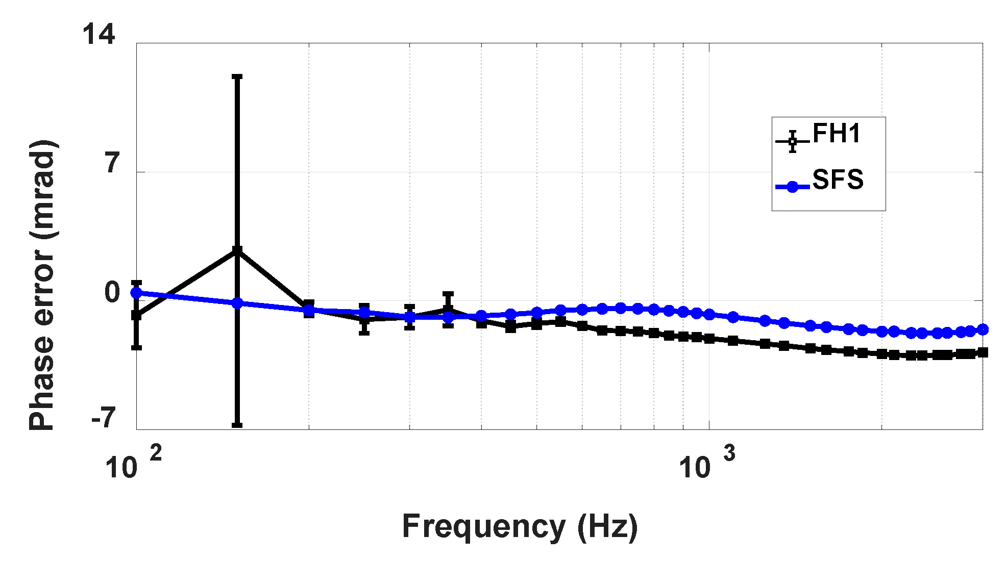
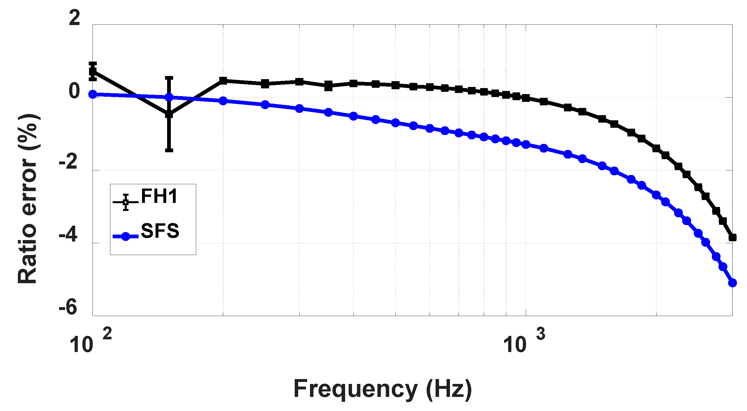
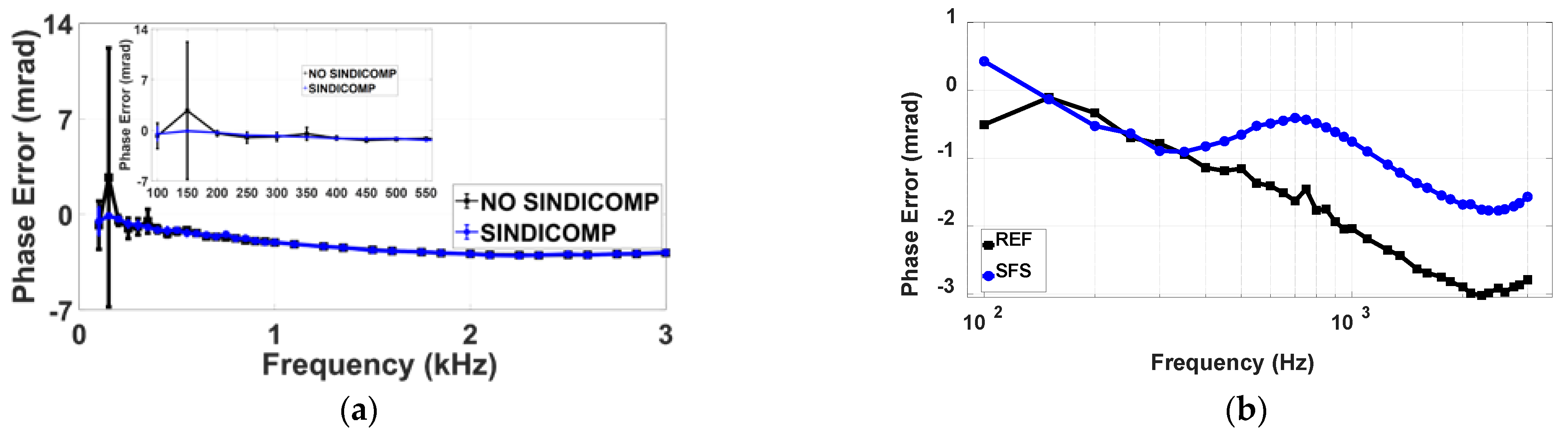
Figure 1 and Figure 2 show, respectively, the ratio and the phase errors of the considered VT, obtained with:

• Waveforms composed by a fundamental tone, at 50 Hz and rated amplitude and a harmonic tone with fixed amplitude (1% of fundamental tone) and variable frequency and phase angle (in the following, this kind of test will be referred to as FH1, that stands for Fundamental and one Harmonic tone). Here, SINDICOMP is not yet applied.
• Sine waves with reduced amplitude (40 V) and variable frequency (in the following, this kind of test will be referred to as SFS, which stands for Sinusoidal Frequency Sweep).

The first thing that can be observed is the presence of the bars on the FH1 curves, both ratio and phase errors: they show here the variability of the ratio and phase errors when the relative phase angle between the fundamental and each harmonic tone changes in the range −π to π, as detailed in [7].

As regards the ratio error, the SFS and FH1 curves are always distant and the maximum difference is about 1.3%. For the phase errors, with the exception of the second and the third harmonic where a strong non-linearity is observed, they have a quite similar behavior, with a maximum absolute deviation of about 1.4 mrad.

To significantly reduce the bars on the FH1 curves, the application of SINDICOMP represents a possible solution. Nevertheless, SINDICOMP aims at compensating the VTs non-linearity errors at the first harmonics and it is not intended for the estimation and compensation of the VT error due to linear effects at frequency higher than 500–750 Hz. To this purpose, the current state of art suggests to perform complex characterization techniques [4,5,6,7,8,9,10] that require the use of complex generation and measurement setups. In this scenario, E-SINDICOMPS aims at:

• using SINDICOMP to compensate for the non-linearity effects;
• proposing an extension to SINDICOMP for the evaluation of the linear effects of VTs using low voltage sinusoidal waveforms, so avoiding using complex characterization techniques as in [4,5,6,7,8,9,10].

An exhaustive description of E-SINDICOMP is given in the following subsections.

3.2. First Step: Non Linearity Compensation

The first step of E-SINDICOMP consists in the application of SINDICOMP [7]. For sake of clarity, here a brief recall of SINDICOMP is given, whereas a thorough description can be found in [7].

Due to the core non-linearity, even if a VT is supplied with a sinusoidal input, the secondary voltage is distorted by the introduction of spurious harmonic components due to the distorted magnetization current absorbed by the VT. Thus, according to [7], a primary voltage phasor at each harmonic h can be expressed as:

$${\overline{V}}_{p,h}^d={\overline{V}}_{s,h}^d+{\dot{Z}}^{*}\times {\overline{I}}_{m,h}={\overline{V}}_{s,h}^d-{\overline{V}}_{s,h}^{sin}$$

(1)

where

• the subscripts “p” and “s” stand for primary and secondary side respectively;
• the primary quantities are here referred to the primary side of the transformer, so that the transformation ratio does not explicitly appear (that is the quantities at the secondary side are multiplied by the rated ratio of the VT);
• ${\dot{Z}}^{*}$ and ${\overline{I}}_{m,h}$ are, respectively, the equivalent VT leakage series impedance and the h-harmonic component of the magnetization current;
• the superscript “d” and “sin” refer to tests performed under distorted and sinusoidal conditions.

It is important to emphasize that Equation (1) should be evaluated for a certain number of primary voltage amplitudes included in the operating input range of the VT, that, according to [20], is between 80% and 120% of the rated VT voltage. In other words, to properly reduce the VT non-linearity through SINDICOMP, a number of compensating phasors, one for each tested primary voltage, should be available.

The secondary voltage harmonic components (${\overline{V}}_{s,h}^{sin}$ amplitude and phase), measured under power frequency sinusoidal conditions, can then be used as a correction for the harmonic component ratio and phase error, due to VT non-linearity, when the VT operates under distorted conditions.

Therefore, the first step of E-SINDICOMP consists of just sinusoidal tests performed at power frequency with the voltage amplitudes indicated by the standard [20], i.e., at various values from 80% to 120% of the rated voltage of the VT under test. The measurement is performed at zero and rated burden. In this test, the ratio and phase errors at power frequency, but also the first $N_h$ harmonic phasors introduced by the VT at its output, because of its non-linear behavior, are measured.

Non-linearity effects are significant in a limited harmonic frequency range (e.g., up to the 10–15th harmonic order). With the increase of the frequency, depending on the characteristics and rated primary voltage of the VT, the frequency behavior of the VT is dominated by the winding stray capacitances.

By applying the compensation illustrated in (1), the non-linearity errors are strongly reduced and, therefore, the VT behavior can be considered linear as shown in [7].

It is noteworthy that SINDICOMP can be successfully applied even if the VT is characterized through the use of a high voltage generator not able to supply a spectrally pure high voltage sine waveform, that is a not trivial requirement, especially at MV-HV levels. In fact, it must be considered that: (1) typical total harmonic distortions (THDs) of commercial generators are a small fraction of the percent, so that the harmonic components are very small compared to the fundamental amplitude; (2) under the hypothesis of large fundamental tone and small harmonic tones, as demonstrated in [7], the distortion introduced at the secondary side by the VT non-linearity is mainly dependent only on the fundamental primary tone. Thus, measuring the distortion also at the primary side allows for the identification, at the secondary side, of the harmonic tones introduced by the VT intrinsic non-linearity from those due to the used generator.

3.3. Second Step: Approximated Voltage Transformer (VT) Frequency Response

The second step of the procedure consists in the execution of SFS test (as defined in Section 3.1), using low voltage sine waves $V_{low}$ (from some volt up to a few hundred volt) at harmonic frequencies (i.e., starting from the second harmonic, since the ratio and phase error at fundamental frequency has been determined in the first step). For each test frequency, ratio and phase errors are evaluated according to:

$${\epsilon }_{h_{\%}}=\frac{k_r{V}_{s,h}-V_{p,h}}{V_{p,h}}\times 100$$

(2)

$${\phi }_h={\phi }_{s,h}-{\phi }_{p,h}$$

(3)

where

• $k_r=\raisebox{1ex}{$V_{p,r}$}\!\left/ \!\raisebox{-1ex}{$V_{s,r}$}\right.$ is the rated transformation ratio ($V_{p,r}$ and $V_{s,r}$ are the rated primary and secondary voltages);
• $V_{p,h}$ and $V_{s,h}$ are the root mean square (rms) values of the primary and secondary h-order harmonic voltage;
• ${\phi }_{p,h}$ and ${\phi }_{s,h}$ are phase angles of the primary and secondary h order harmonic voltage.

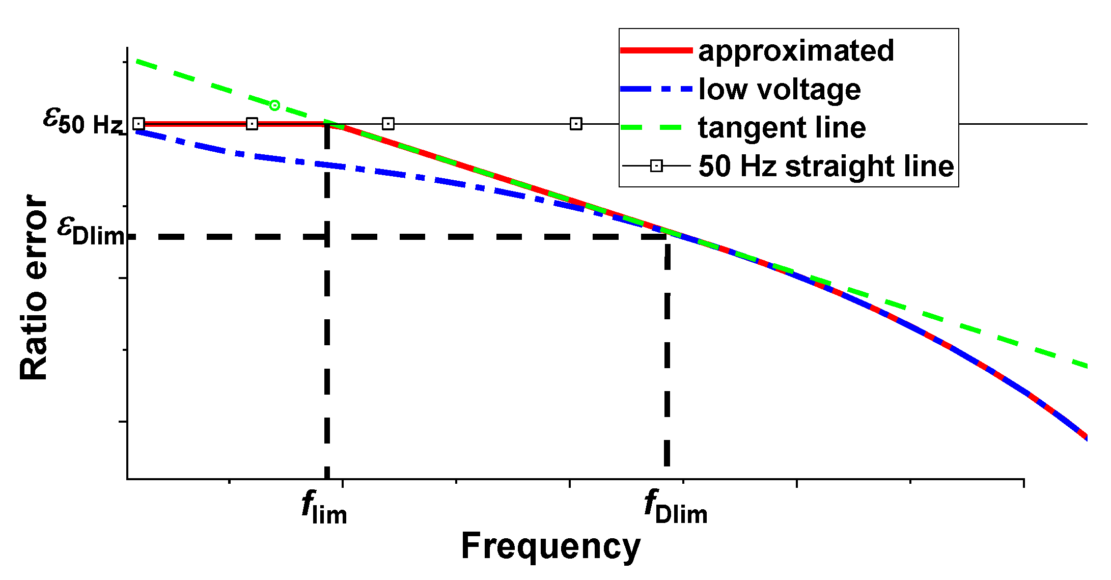
The approximated VT frequency response is constructed starting from three different curves: (1) the response measured at power frequency (from now on referred to as 50 Hz, being intended that the validity of the method remains even if a different value applies) (2) the low voltage response and (3) the low voltage response tangent. Three different frequency regions are defined and, in each region, a different curve is used to approximate the actual VT response.

The proposed approach is synthesized in Figure 3, where the ratio errors versus frequency are shown.

In the first region, that is from 50 Hz up to the frequency $f_{lim}$, a flat frequency response can be assumed basing on the consideration that the frequency response of a VT, after the compensation of non-linearity error, is quite flat up to some hundreds of hertz. Therefore, the ratio error is assumed constant and assumed equal to that measured at 50 Hz (${\epsilon }_{50\mathrm{Hz}}$), up to the limit frequency $f_{lim}$:

$$\epsilon \left(f\right)={\epsilon }_{50\mathrm{Hz}}, 50 \mathrm{Hz}<f< f_{lim}$$

(4)

The frequency $f_{lim}$ is defined as the intersection frequency between the flat line $\epsilon \left(f\right)={\epsilon }_{\left(50\mathrm{Hz}\right)}$ and the straight line $\tau \left(f\right)$ with negative slope $D_{lim}$, which is tangent in $f_{Dlim}$ to the ratio error curve ${\epsilon }_{LV}\left(f\right)$, measured at low voltage. Therefore, the second region is identified from the frequencies $f_{lim}$ and $f_{Dlim}$ and the ratio error is assumed equal to $\tau \left(f\right)$ as:

$$\begin{gathered} \epsilon \left(f\right)=\tau \left(f\right), f_{lim}<f< f_{Dlim} \\ \tau \left(f\right)=D_{lim}\times \left(f-f_{Dlim}\right)+{\epsilon }_{Dlim} \\ {D}_{lim}={\left.\frac{d{\epsilon }_{LV}}{df}\right|}_{f=f_{Dlim}} \end{gathered}$$

(5)

Since $f_{lim}$ is the frequency where $\tau \left(f\right)$ is equal to ${\epsilon }_{50\mathrm{Hz}}$, $f_{lim}$ Equation (6) results:

$$f_{lim}=f_{Dlim}+\frac{{\epsilon }_{50\mathrm{Hz}}-{\epsilon }_{Dlim}}{D_{lim}}$$

(6)

Obviously, other possible curves can be used for the second frequency region; however, since this paper aims to propose a simplified technique, a straight line is the simplest solution.

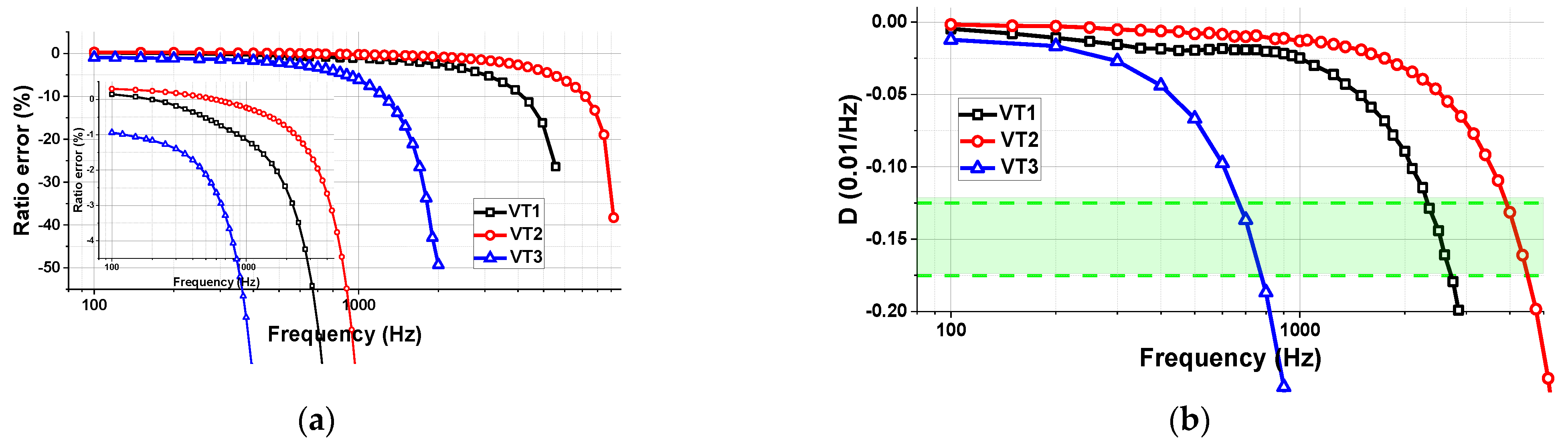
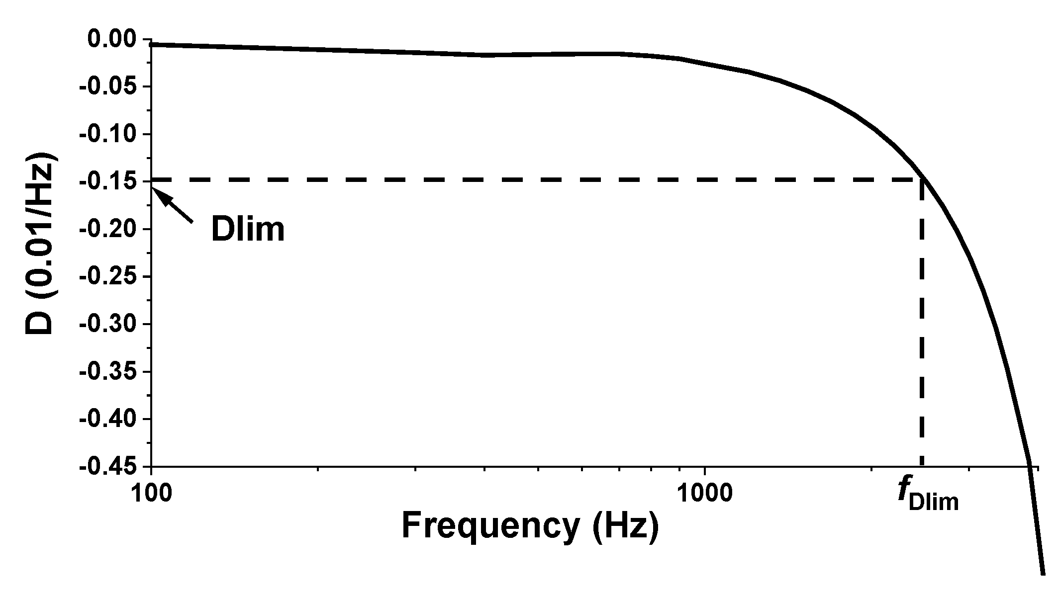
The identification of the frequency $f_{Dlim}$ is based on the analysis of the frequency behavior of the derivative D of the low voltage ratio error ${\epsilon }_{LV}$. Preliminary experimental tests on MV VTs with different features and primary voltage from 6 kV up to 20 kV have demonstrated that D has a quite repetitive behavior, shown in Figure 4: after a first flat part, the curve starts to decrease and from a certain frequency point, identified as $f_{Dlim}$, the absolute value of the negative slope significantly increases.

The study of the shape of D allows the discrimination of the frequency behavior of the VT. More specifically, the first flat part can be associated with the non-linear behavior of the VT whereas the region from $f_{Dlim}$, where the D slope becomes higher, can be associated with the increasing weight of the winding stray capacitances. According to this, for frequencies higher than $f_{Dlim}$ the predominance of the linear effects allows us to state that the VT error behavior at rated primary voltage and that measured at low voltage are overlapped.

According to experience gained in the experimental tests, the value of $D_{lim}$ ranges between −0.10 (0.01/Hz) to −0.2 (0.01/Hz). Additionally, information on the numerical selection of the optimum $D_{lim}$ and, thus, on the frequency $f_{Dlim}$ are provided in Section 5.2.

The third region is defined for frequencies higher than $f_{Dlim}$ and the ratio error $\epsilon \left(f\right)$ is assumed equal to the ratio error ${\epsilon }_{LV}\left(f\right)$ measured at low voltage:

$$\epsilon \left(f\right)={\epsilon }_{LV}\left(f\right), f>f_{Dlim}$$

(7)

Regarding the phase response, the use of the SFS phase response gives acceptable results, as it can be observed in Figure 2 and in the figures shown in Section 5.

4. Measurement Setup

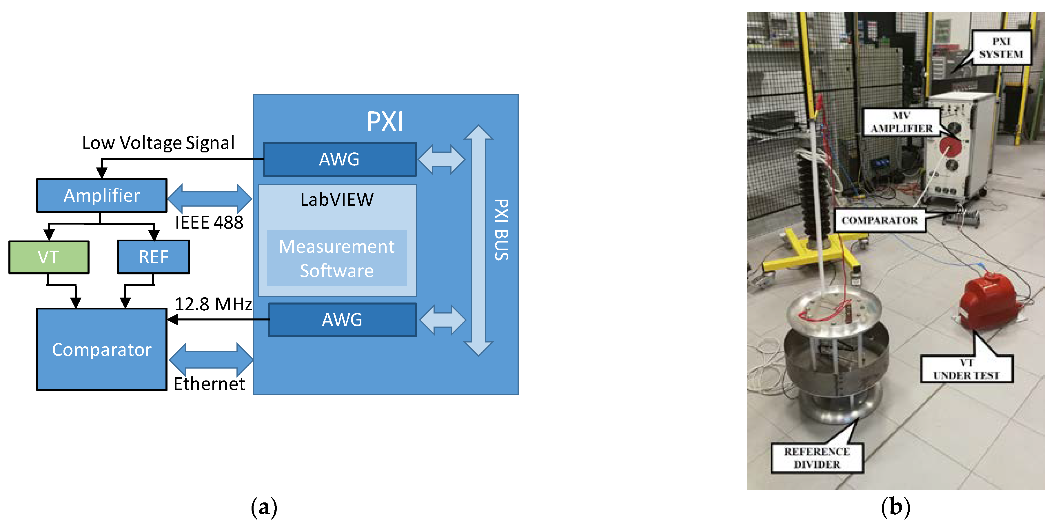
The setup used for VT characterization is shown Figure 5: Figure 5a shows the block diagram, whereas Figure 5b shows the INRIM generation and measurement circuits. The low voltage signal is generated by an Arbitrary Waveform Generator (AWG), the National Instruments (NI) PCI eXtension for Instrumentation (PXI) 5422, with 16 bit, variable output gain, ±12 V output range, 200 MHz maximum sampling rate, 256 MB onboard memory. It is inserted in a PXI chassis and the 10 MHz PXI clock is used as reference clock for its Phase Locked Loop (PLL) circuitry. The generation frequency of the AWG is therefore chosen to be an integer multiple of the generated fundamental frequency. The voltage waveform generated by the AWG is amplified by a Trek high-voltage power amplifier (30 kV, 20 mA, peak values) with wide bandwidth (from DC to 2.5 kHz at full voltage and 30 kHz at reduced voltages), high slew rate (<550 V/µs) and low noise. Applied voltage reference values are obtained by means of a 30 kV wideband reference divider designed, built and characterized at INRIM [23].

The acquisition system is obtained through a NI cDAQ chassis with four different acquisition modules: NI 9225 (±425 V, 24 bit, 50 kHz), NI 9227 (±14 A, 24 bit, 50 kHz), NI 9239 (±425 V, 24 bit, 50 kHz), NI 9238 (±500 mV, 24 bit, 50 kHz) [24]. The sampling clock of the comparator is derived from the 12.8 MHz time base clock, provided by a second AWG (Figure 5a). In this way, generation and acquisition are precisely synchronized.

The VT primary and secondary voltages are acquired with a sampling frequency f_s equal to 50 kHz, the time window chosen is 1 s and ten repetitions are executed for each test. The Discrete Fourier Transform (DFT) is performed on the acquired samples and the phasors of the voltages at VT primary and secondary side are measured.

The overall relative uncertainty (level of confidence 95%) of the measurement setup in Figure 5 ranges from 70 µV/V and 70 µrad at 50 Hz up to 200 µV/V and 350 µrad at 9 kHz for the ratio and phase error, respectively.

5. Application of E-SINDICOMP to Various Voltage Transformer (VTs)

The described procedure is experimented measuring the frequency behavior of three MV VTs for substation indoor applications. For each considered VT, the validity of the proposed approach is investigated by carrying out measurements of the frequency behavior on the same VT at low voltage and at MV up to the first resonance frequency [25]. In particular, the FH1 test, along with the application of SINDICOMP, has been used to obtain the reference frequency behavior (hereinafter REF), whereas E-SINDICOMP has been used to build the approximated one.

The VTs considered in this analysis are commercial resin insulated VTs for MV phase-to-ground 50/60 Hz measurements.

Table 1. Features of the investigated Voltage Transformers (VTs).

Name	Primary Voltage (kV)	Secondary Voltage (V)	Rated Burden (VA)	Accuracy Class	First Resonance Frequency fr (kHz)
VT1	20/√3	100/√3	50	0.5	5.5
VT2	11/√3	110/√3	50	0.5	9.2
VT3	20	100	50	0.2	2.0

summarizes the features of the considered transformers.

5.1. Test Description

The FH1 test is performed by using a fundamental tone with 80%, 100% and 120% of the VT rated amplitude, frequency 50 Hz and zero phase. The harmonic tone has amplitude of 1% of the fundamental tone, phase variable in the range −π ÷ π and order from 2nd to 180th. The measurements are performed with both rated and zero burden and applying SINDICOMP to obtain REF.

Then, E-SINDICOMP is applied to the VT. As for REF, also in this case the measurements are performed with both zero and rated burden; however, for sake of brevity, Section 5.2, Section 5.3, Section 5.4 and Section 5.5 show results related to the measurements with zero burden, whereas the effect of burden is discussed in Section 5.6. In the first step, the VT is characterized through SINDICOMP, that is by applying sine waves having 80%, 100% and 120% of the rated primary voltage at 50 Hz frequency [20]. Ratio and phase error at 50 Hz are evaluated and the harmonic phasors at the VT output are measured up to 1 kHz.

In the second step, a SFS test is carried out, using sine waves with amplitude 40 V and frequency from 100 Hz up to the VT first resonance frequency; for each test frequency, the ratio and phase errors are measured. From the SFS data, the $D_{lim}$ and $f_{Dlim}$ parameters are evaluated by following the procedure described in the Section 5.2 and the approximated frequency response (APP) is built.

To assess the performance of the proposed E-SINDICOMP technique, the obtained results are compared with the reference response REF.

Measurements described above are carried out under controlled environmental conditions (temperature 23 ± 1 °C, relative humidity in the range 40% to 70%).

5.2. Identification of the D_lim Value

Following the considerations given in Section 3.3, is was experimentally determined that the values of $D_{lim}$, for all the analyzed VTs, can be found in the range −0.10 (0.01/Hz) to −0.2 (0.01/Hz). We recall here that the quantity $D_{lim}$ identifies a frequency point, $f_{Dlim}$, after which the behavior of the VT can be considered linear.

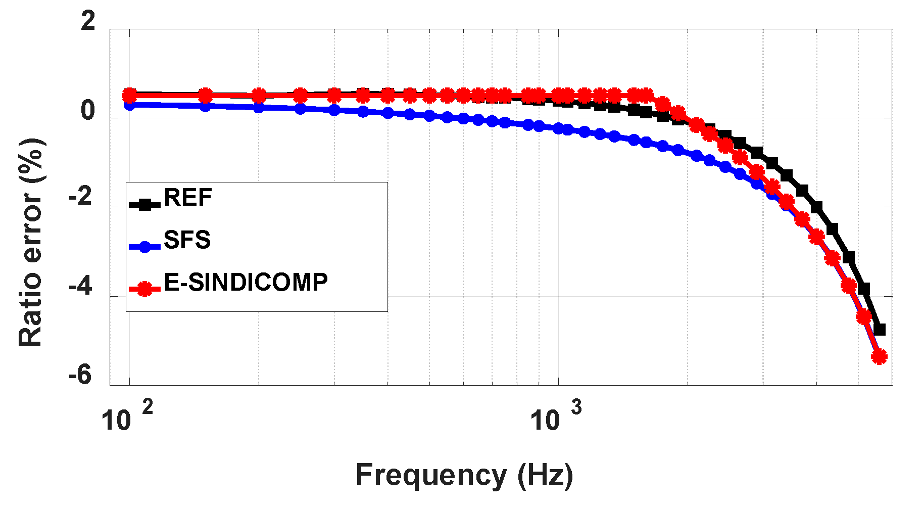
For the three analyzed VTs, the optimum $D_{lim}$ values were identified by analyzing the derivative of the VTs SFS frequency responses (ratio error), measured at low voltage (40 V). Figure 6a shows the three SFS ratio error curves up to the respective resonance frequency and a zoom up to the respective frequency $f_{Dlim}$. Figure 6b shows, instead, their derivative curves $D$: the highlighted green portion, that is from 0.12 to 0.16 (0.01/Hz), locates for all the three curves the region where the absolute value of the slope starts to significantly increase.

Table 2. Selected $D_{lim}$ and $f_{Dlim}$ values of the investigated Voltage Transformer (VTs).

DUT	${\mathit{D}}_{\mathit{l}\mathit{i}\mathit{m}}$ (0.01/Hz)	$$\begin{gathered} {\mathit{f}}_{\mathit{D}\mathit{l}\mathit{i}\mathit{m}} \\ \mathbf{\left(}\mathbf{Hz}\mathbf{\right)} \end{gathered}$$	$$\begin{gathered} {\mathit{f}}_{\mathit{l}\mathit{i}\mathit{m}} \\ \mathbf{\left(}\mathbf{Hz}\mathbf{\right)} \end{gathered}$$
VT1	−0.15	2500	800
VT2	−0.14	4000	1600
VT3	−0.14	800	300

shows the $D_{lim}$ and $f_{Dlim}$ selected values for the investigated VTs.

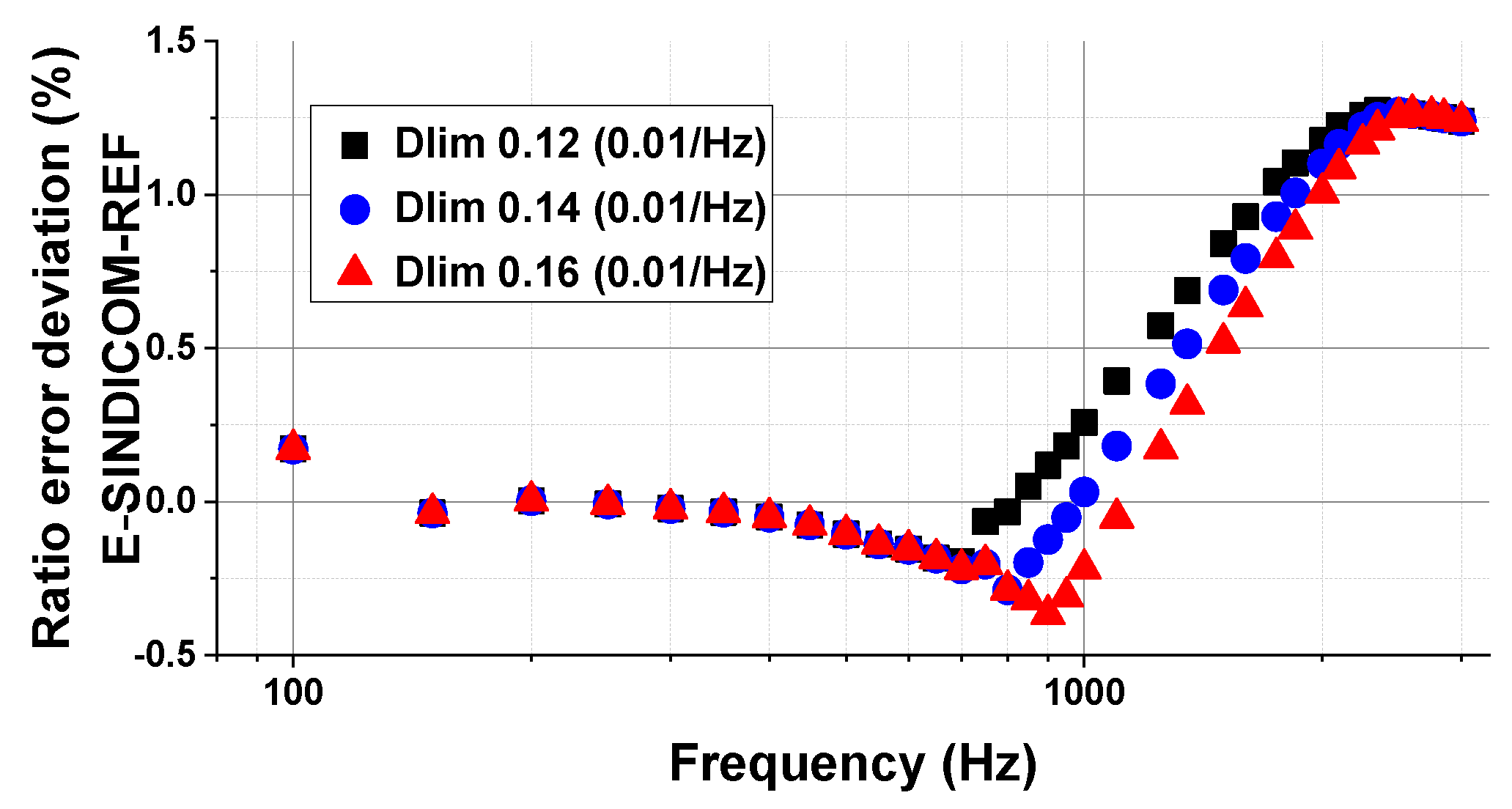
Looking at Figure 6b, it can be noted that for VT1 three different $D_{lim}$ values are included in the considered range. Therefore, to assess the impact of the $D_{lim}$ selection on the performance of E-SINDICOMP, the technique is performed for all three values. Three E-SINDICOMP responses are built for each of the three $D_{lim}$ values, 0.12, 0.14 and 0.16 (0.01/Hz), that respectively correspond to $f_{Dlim}$ values of 2350 Hz, 2500 Hz and 2600 Hz. As regards the $f_{lim}$ frequency, the three $f_{Dlim}$ values identify three different $f_{lim}$ values equal to 700, 800 and 900 Hz, respectively.

Figure 7 shows the results of this analysis, depicting, in particular, the ratio error deviations between the REF curve and the three E-SINDICOMP responses, which are obtained for the different $D_{lim}$ and $f_{Dlim}$ values.

As it can be observed, the three curves are well overlapped below the lowest $f_{lim}$ value, that is 700 Hz. From this frequency point, the three curves are distanced (maximum deviations of 5 mV/V among them) and the best result is obtained with $D_{lim}$ = 0.14 (0.01/Hz), identified by circle markers in Figure 7. After 2.6 kHz, that is the higher $f_{Dlim}$ value, the three curves come closer together, resulting again overlapped. As such, for the rest of the analysis, a $D_{lim}$ = 0.14 (0.01/Hz) is chosen for VT1.

5.3. VT 1 Characterization

For VT1, some experimental results have been already presented in Section 3 and Section 5.2. Here, the complete characterization is shown.

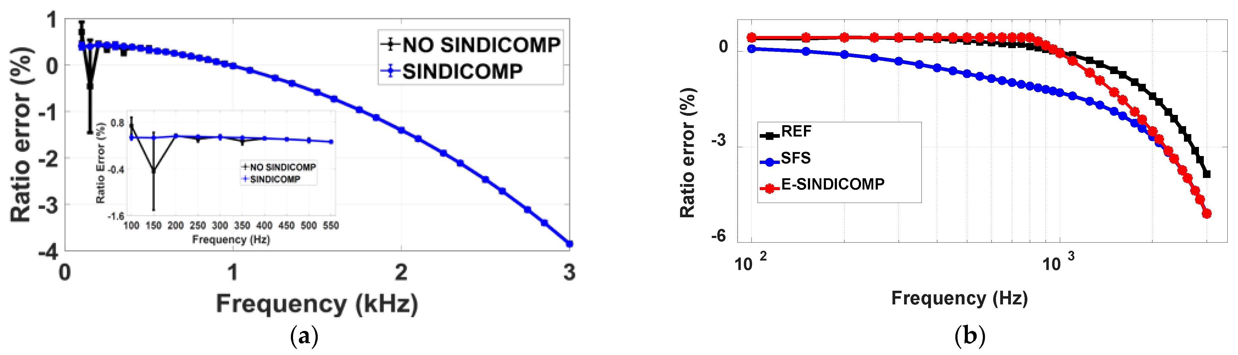
Figure 8a, Figure 9a shows the comparison between the FH1 ratio errors (phase errors) obtained with and without the application of SINDICOMP; it is worth to recall that FH1 with SINDICOMP corresponds to REF frequency behavior. Each frequency point is obtained averaging the ratio errors (phase errors) over the −π ÷ π phase variation range of the harmonic tones; the bars, instead, represent the maximum deviation of the errors over the same phase variation range. The amplitude of the bars represents an index of the non-linearity of the VT at a specific frequency [7]. Figure 8a and Figure 9a also shows in the inset a zoom of the low frequency region, up to 550 Hz.

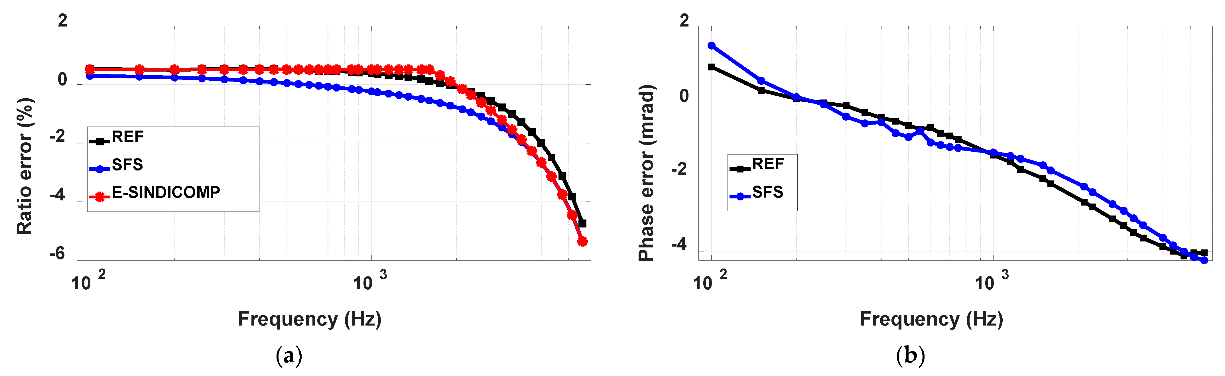
All the three ratio error curves, the REF, the SFS and the E-SINDICOMP are finally shown in Figure 8b. The same curves, but related to phase error, are shown in Figure 9b, recalling that E-SINDICOMP phase error is equal to SFS phase error; Figure 9b also shows the 50 Hz phase error.

Finally,

Table 3. VT1: deviations between SFS and REF responses and between E-SINDICOMP and REF responses.

Frequency (Hz)	Ratio Error Deviation (%)		Phase Error Deviation (mrad) SFS-REF
	SFS-REF	E-SINDICOMP-REF
100	−0.36	0.03	0.93
200	−0.54	−0.0039	−0.19
300	−0.72	0.022	−0.11
700	−1.19	0.22	1.22
1000	−1.27	−0.031	1.28
1250	−1.28	−0.38	1.26
1500	−1.29	−0.69	1.26
1750	−1.29	−0.93	1.20
2000	−1.27	−1.0	1.21

shows the deviations, on ratio and phase errors, obtained between SFS and REF responses and between E-SINDICOMP and REF responses. It is worthwhile noting that, for the phase response, SFS and E-SINDICOMP coincide. Good improvements, up to one order of magnitude for the ratio error deviations up to hundreds of hertz, are obtained by using the E-SINDICOMP frequency response with respect to the use of the SFS response.

5.4. VT2 Characterization

The second VT (VT2) has been selected with a primary voltage half of the VT1 one, same manufacturer, lower transformation ratio (100 against 200) and higher first resonance frequency (9.2 kHz against 5.5 kHz).

Figure 10a,b show the comparison of the REF, the SFS and the E-SINDICOMP ratio and phase errors, respectively.

Table 4. VT 2: deviations between SFS and REF responses and between E-SINDICOMP and REF responses.

Frequency (Hz)	Ratio Error Deviation (%)		Phase Error Deviation (mrad) SFS-REF
	SFS-REF	E-SINDICOMP-REF
100	−0.24	−0.03	0.57
500	−0.47	−0.01	−0.31
1000	−0.62	0.12	0.07
1500	−0.68	0.31	0.35
2000	−0.69	−0.01	0.41
2500	−0.69	−0.21	0.39
3000	−0.69	−0.43	0.38
3500	−0.67	−0.56	0.34

shows the deviations, on ratio and phase errors, obtained between SFS and REF responses and between E-SINDICOMP and REF responses. Again, as already seen for VT1, E-SINDICOMP gives good results compared to the use of SFS.

5.5. VT3 Characterization

The third investigated VT, VT3, is a resin insulated transformer from a different manufacturer. It has higher primary voltage and two different ratios, 50 kV/100 V and 20 kV/100 V; here, only the 20 kV/100 V configuration was used.

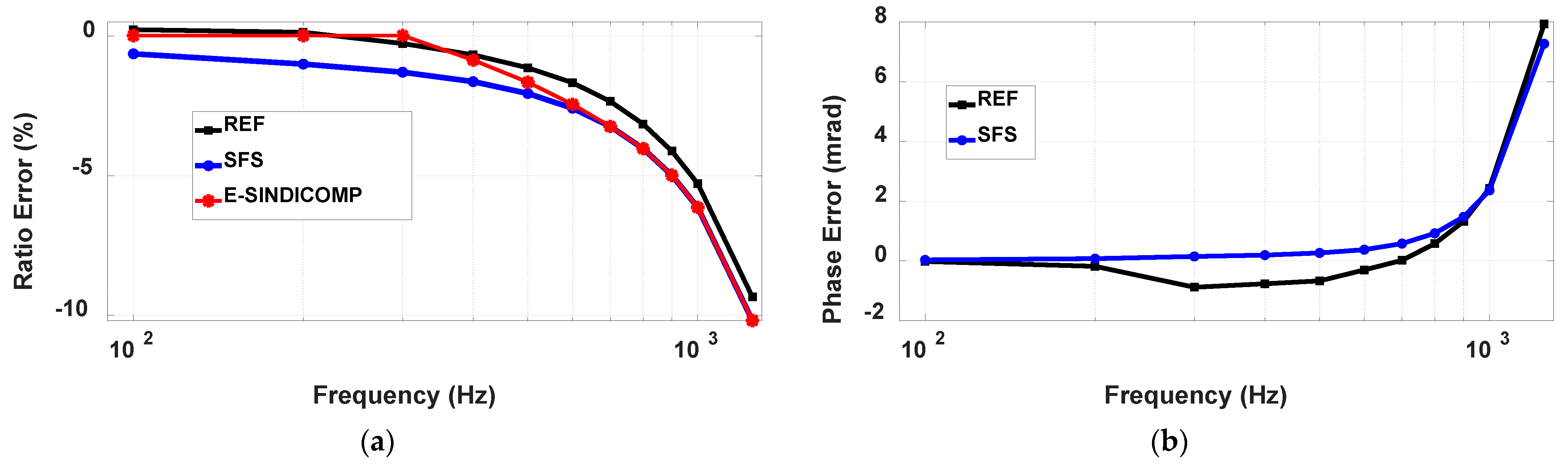
As in the previous cases, Figure 11a,b show the comparison among the REF, the SFS and the E-SINDICOMP ratio and phase errors, respectively, whereas the deviations with respect to REF are quantified in

Table 5. VT3: deviations between SFS and REF responses and between E-SINDICOMP and REF responses.

Frequency (Hz)	Ratio Error Deviation (%)		Phase Error Deviation (mrad) SFS-REF
	SFS-REF	E-SINDICOMP-REF
200	−0.86	−0.21	−0.052
300	−1.14	0.120	−0.27
500	−0.96	−0.19	−1.03
700	−0.91	−0.77	−0.56

.

As can be observed, even if the rated transformation ratio is the same of VT1, the frequency response is different since the first resonance frequency is quite lower (about 2 kHz against 5.5 kHz). This can be explained considering that VT3 has a higher primary voltage (20 kV against 20/√3 kV), so a higher number of primary turns and then a higher stray capacitance, which implies a lower resonance frequency. Considering the results given in Figure 11, also in this case, the adoption of the selection criteria identified for $D_{lim}$ and $f_{Dlim}$ gives quite good results in the identification of the linear portion of the approximated curve for the working out of the approximated behavior.

5.6. Burden Effect

The scope of this section is to evaluate the effect of the VT burden on the E-SINDICOMP performance. For sake of brevity, here only the results related to VT2 at rated burden, i.e., 50 VA, are shown, but similar considerations also apply for the other two VTs.

By the study of the derivative $D$ of the VTs SFS, measured in presence of the rated burden, $f_{Dlim}$ is set to 4350 Hz which corresponds to $D_{lim}$ equal to 0.16 (0.01/Hz) whereas $f_{lim}$ is set to 1500 Hz.

Comparing the resulting values of $f_{lim}$ and $f_{Dlim}$ (1500 Hz and 4350 Hz) with the values obtained under zero burden conditions (1600 Hz and 4000 Hz), an enlargement of the second frequency region can be noticed.

Results related to burden effect on E-SINDICOMP performance are shown in Figure 12 where the ratio errors corresponding to REF, SFS and E-SINDICOMP are compared.

Similarly, to the zero burden case, the E-SINDICOMP method strongly reduces the ratio error deviations, by giving values below 0.1% up to 1 kHz, whereas the maximum error is found at 4350 Hz and equal to −1.1%.

6. Conclusions

This paper has presented a simplified technique for the frequency characterization of MV VTs, which can be executed using only sine waves. It is thought to be simple and to require instrumentation that is typically already available in VT calibration laboratories, including the laboratories of the VT manufacturers. The proposed technique is called E-SINDICOMP, since it extends and integrates the SINDICOMP technique, already presented by some of the authors. The main advantages of this technique are summarized as follows.

• E-SINDICOMP requires two measurement steps for the frequency characterization of MV VTs, the first of which, executed at power frequency, is identical to the standard procedure for VT calibration [20], so that every VT calibration laboratory is able to perform it.
• The second measurement step involves the generation and measurements of sine waves at some tens of volt and up to some kilohertz, again requiring measuring instrumentation generally available in most electrical measurement laboratories.
• E-SINDICOMP has been applied to three different commercial MV VTs, showing a good performance improvement with respect to the use of the widely adopted low voltage sinusoidal frequency sweep technique.

As a final consideration, it can be noticed that the frequency behavior of a MV VT evaluated by E SINDICOMP can allow, by compensation of the VT errors, a significant improvement in the accuracy of harmonic measurements, especially in the frequency range where the VT response is mainly affected by the non-linear effects and in the transition region between non-linear and linear behavior.