Robust Control of a PMSG-Based Wind Turbine Generator Using Lyapunov Function

Abstract

This paper proposes a robust finite-time controller (FTC) for a permanent magnet synchronous generator (PMSG)-based wind turbine generator (WTG). An adaptive observer is used for the rotor angle, rotor speed, and turbine torque estimations of the PMSG, thus eliminating the use of anemometers. The robustness of the proposed FTC regarding parameter uncertainty and the external weak power grid is analyzed. The impacts of the power grid short-circuit ratio (SCR) at the point of common coupling (PCC) on the conventional proportional-integral (PI) controller and the proposed FTC are discussed. Case studies illustrate that the proposed observer-based FTC is able to estimate the mechanical variables accurately and provides robust control for WTGs with parameter uncertainty and weak power grids.

1. Introduction

The control and integration of wind energy into a power grid are challenging due to geographical constraints and the intermittency of energy production. The maximum power point tracking (MPPT) control plays a vital role in maximizing the wind energy yield from wind turbines [1]. Wind-characteristic-based MPPT methods require online wind speed and mechanical torque measurements using mechanical sensors, e.g., an anemometer installed at a nacelle [2]. Sensorless controls of wind turbine generators (WTGs) can eliminate expensive mechanical sensors and improve the reliability of the WTGs [3,4,5]. Sensorless controls can also facilitate sensor fault detection and isolation when mechanical sensors are present [6].

Kalman filters can be used for rotor position and speed observations of WTGs [4]. However, Kalman filters are based on linearized models of the nonlinear WTG system [7]; thus, they are not suitable for WTGs at low speeds with small back electromotive forces (EMFs). Rotor position observation through high-frequency signal injection is also challenging at high speeds [8]. Artificial neural network (ANN)-based sensorless controls are proposed in [9,10], which requires extensive offline data collection and training to achieve nonlinear input–output mapping. In [11], the rotor position is estimated using a phase-locked loop (PLL). Back EMF-based PLL observers have been studied for sensorless control of permanent magnet synchronous motors (PMSMs) to estimate the position/speed of the rotor [12,13]. A PLL combined with synchronous frequency-extract filters was proposed in [12] to mitigate the estimated back EMF harmonic error in the sensorless control of surface PMSMs. In [13], a new finite-position set–PLL (FPS-PLL) based on model predictive control was investigated, where the rotor position was identified from the finite set of rotor positions. The consequences demonstrated excellent performance in estimating the position/speed of the rotor in the FPS-PLL compared to the conventional PLL, as well as a significant reduction in dynamic and steady-state fluctuations. Two computationally efficient finite-position set–PLL were proposed in [14] to diminish the computational effort of the FPS-PLL proposed in [13].

Sliding-mode observers for PMSM sensorless controls have been extensively surveyed [15,16,17,18,19,20]. A wind speed estimation and sensorless control for a surface-mounted permanent magnet synchronous generator (PMSG) using sliding mode control (SMC) based on a linear matrix inequality (LMI) was proposed in [15], in which the rotor speed is estimated according to the rate of change in the estimated rotor position. In [19] and [20], the estimations of the rotor position and the stator flux linkage were investigated using a quasi-sliding mode observer and a model reference adaptive system using an sliding mode observer (SMO). However, the turbine mechanical torque was not estimated in [11,19,20]. Additionally, the maximum back EMF and the sampling frequency impose constraints on the convergence of the quasi-sliding mode observer [19]. In [21,22], second-order sliding mode (SOSM) control for a doubly fed induction-generator-based wind turbine has been discussed. This control method improves the classical sliding mode (first-order) chattering problem. Moreover, the main features of SOSM control are robustness with respect to perturbations (grid fault) and chattering-free behavior. An adaptive Kalman-like observer was proposed in [23], which can provide accurate and reliable estimations of system states and parameters for a generic nonlinear system. It will be used in the paper for estimations of the rotor speed and the turbine mechanical torque of the WTG system under a wide range of operating conditions.

A linear controller for the WTG is the most widely used control method, e.g., proportional-integral (PI) controllers [24,25,26,27], the fuzzy propotional-integral-derivative (PID) [28], and the self-tuned adaptive PI controller [29]. PI controllers are very common in the industry due to their simple structure and easy implementation in various applications. Such controllers are designed for a single operating point. The operating point changes due to the disturbances and variation in parameters. In this case, the controller will not have a proper performance, and voltage and power oscillations will appear. In addition, such controllers are very sensitive to parameter variations. Hence, an accurate mathematical system model is required to determine the control parameters. However, accurate calculation of the system model is not possible due to unknown machine and environment parameters, core saturation, wind oscillations, temperature variations, and system disturbances [8,24,25].

A linear controller is fundamental to the stable and reliable operation of the WTG system. Connecting the WTG system to a weak power grid represents challenges and requires detailed stability analysis of the WTG and the power grid [30]. The inherent right half-plane (RHP) zero and pole in the converter’s transfer function are major concerns for the linear controller design of the PMSG-based WTG system when connected to a weak grid [31,32]. Accordingly, root-locus analysis shows that a pole pair enters the RHP and becomes unstable by decreasing the short-circuit ratio (SCR) of the grid [33]. The PLL dynamic also plays a critical role in connecting WTGs to a weak grid [34]. In [35], the power synchronization method was developed to connect an off-shore wind farm to a weak power grid. A three-level hierarchical control scheme was used in [36] to support the point of common coupling (PCC) voltage for connecting the WTG to a weak grid.

Linear controllers are designed under specific operating conditions and are influenced by large external perturbations and parameter uncertainties. Therefore, several nonlinear control techniques are proposed, including the intelligent fuzzy sliding-mode control [37], radial basis function network-based neural network control [38], and adaptive fuzzy control [39]. However, these artificial intelligence control methods require prior behavioral knowledge about the WTG system and extensive training data. Although the nonlinear controllers in [37,38,39,40] led to exponential convergence of the state trajectories, finite-time controller (FTC) architectures [41] can push the control system error trajectories to zero in a pre-defined time, thus resulting in fast convergence of system states, high control accuracy in the steady state, and excellent robustness against perturbations and uncertainties.

This paper proposes a robust FTC method for the PMSG-based WTG system. The nonlinear controls of the machine-side converter (MSC) and the grid-side converter (GSC) are based on the control Lyapunov function (CLF) and back-stepping control design techniques. The main contributions of the paper are summarized as follows:

• A novel back-stepping finite-time controller is proposed for the PMSG-based wind generation system, and its stability and finite-time convergence are proved mathematically using the Lyapunov stability theorem.
• The proposed multi-loop output-feedback nonlinear FTC improves the control robustness against parameter uncertainty by the proper tuning of its control gains. The robustness of the FTC is verified using the perturbed WTG system with 20% parameter variation and a weak power grid at the PCC.
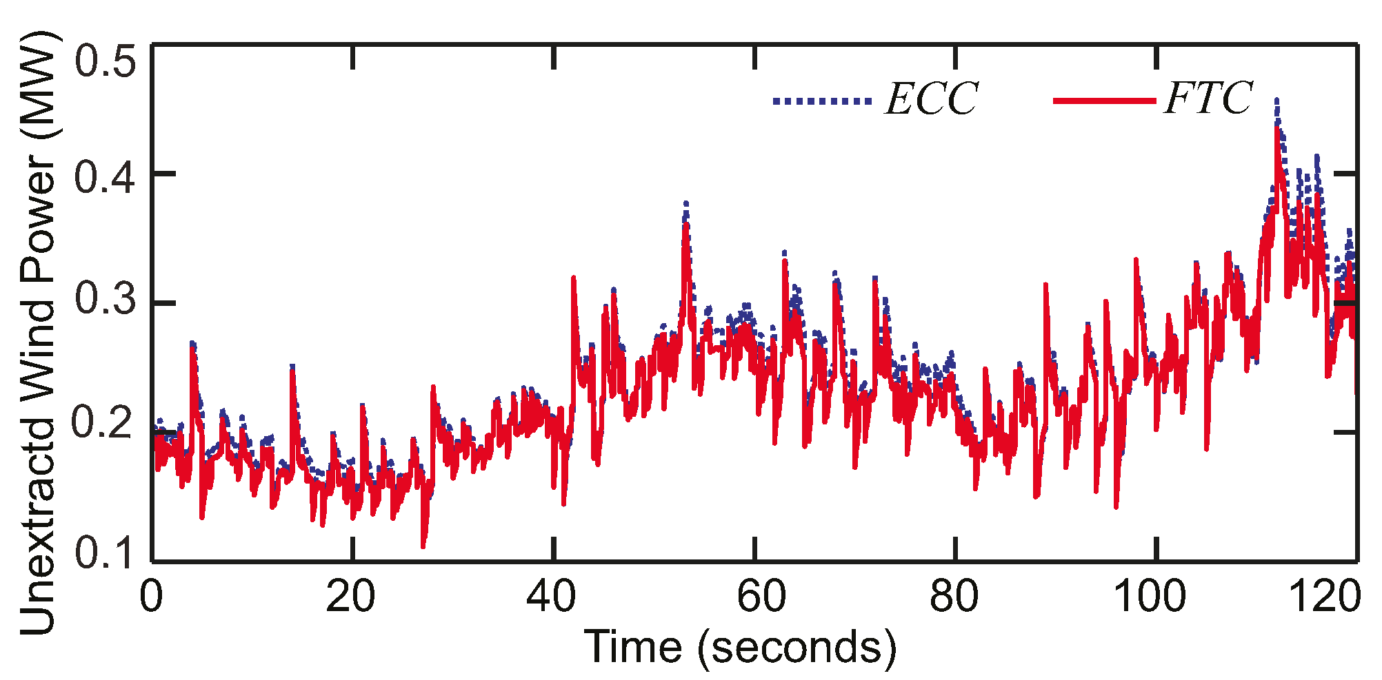
• The proposed FTC leads to fast convergence of the system states and small steady-state errors for normal and perturbed WTG systems with parameter uncertainties. Therefore, the FTC achieves faster maximum power point tracking (MPPT) and extracts more wind power compared to conventional linear and nonlinear controllers.
• An adaptive Kalman-like observer is proposed for the WTG system to estimate the rotor position, rotor speed, and turbine mechanical torque. Thus, the proposed FTC achieves mechanical sensorless control of the WTG and increases the reliability of the WTG system.
• Using the reactive power control loop of the proposed controller, the grid’s voltage stability in a weak grid with a low circuit ratio is investigated.

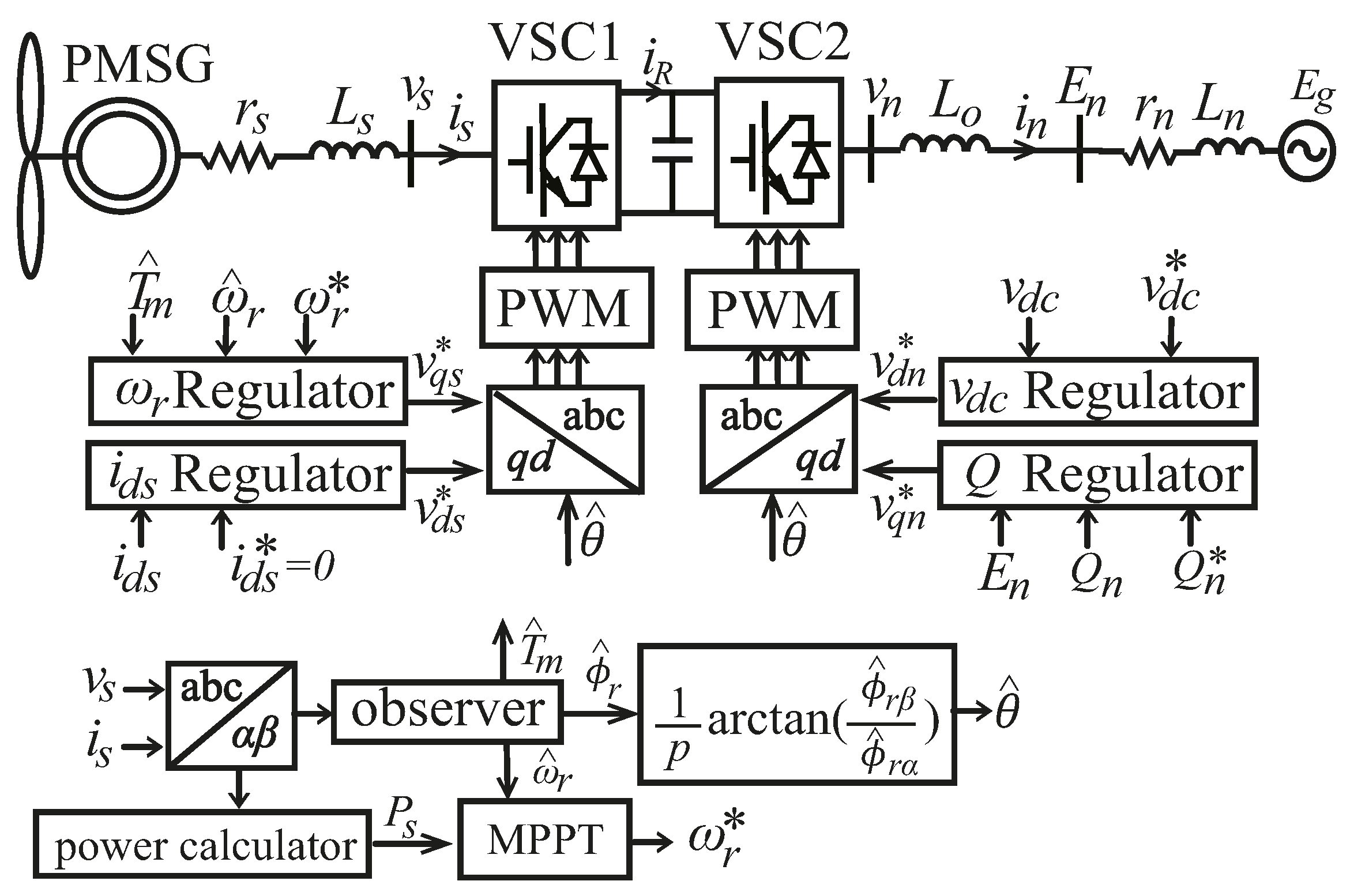
2. PMSG-Based Wind Turbine System Model

The PMSG-based WTG connected to the AC power grid at the PCC, i.e., $E_n$, is shown in Figure 1. The PMSG is connected to the grid through a voltage source converter (VSC) consisting of an MSC and a GSC. The AC power grid is modeled as a voltage source ($Eg$) behind a series branch ($r_n,L_n$). The mechanical power extracted from a wind turbine is calculated as

$$P_m=\frac{1}{2}{c}_p\rho A{v}_w^3$$

(1)

where $c_p=c_p\left(\lambda \right)$, $\lambda =R{\omega }_m/v_w$, R, ${\omega }_m,\rho ,v_w$ and $A=\pi R^2$ are the turbine power coefficient, tip speed ratio, turbine blade, radius, turbine shaft speed, air density, wind speed, and rotor swept area, respectively.

The state–space model of the PMSG-based WTG system in the qd rotor reference frame is expressed as [40]

$$\{\begin{array}{c}\frac{d{\omega }_r}{dt}=-\frac{1}{J}(F{\omega }_r+K_M{i}_{qs}-T_m)\hfill \\ \frac{d{i}_{qs}}{dt}=-\frac{1}{L_s}(r_s{i}_{qs}+L_{s}p{\omega }_r{i}_{ds}-K_M{\omega }_r+v_{qs})\hfill \\ \frac{d{i}_{ds}}{dt}=-\frac{1}{L_s}(r_s{i}_{ds}-L_{s}p{\omega }_r{i}_{ds}+v_{ds})\hfill \\ \frac{d{v}_{dc}^2}{dt}=-\frac{1}{C}(E_{dn}{i}_{dn}+E_{qn}{i}_{qn}-v_{dc}{i}_R)\hfill \\ \frac{d{i}_{dn}}{dt}=-\frac{1}{L_0}(E_{dn}-L_0{\omega }_{\mathrm{n}}{i}_{qn}-v_{dn})\hfill \\ \frac{d{i}_{qn}}{dt}=-\frac{1}{L_0}(E_{qn}+L_0{\omega }_{\mathrm{n}}{i}_{dn}-v_{qn})\hfill \end{array}$$

(2)

where $T_m$ is the turbine mechanical torque, $K_M=p\sqrt{3/2}{\phi }_r$ is the flux generator constant, ϕ_r is the flux generator constant, and i_r is the output DC current of the MSC. The variables and quantities of the WTG system used in the paper are listed in

Table 1. Parameter discription of the wind turbine generator (WTG) model.

Symbol	Quantity	Value
$J$	Rotor inertia	1.06 × 107 Nm/rad/s2
$F$	Viscous coefficient	1.417 Nm/rad/s
$P$	Number of pole pairs	145
$K_M$	Flux generator constant	2.6354 × 103
$r_s$	PMSG stator resistance	3 mΩ
$L_s$	PMSG stator inductance	1 mH
$E_n$	Grid voltage	4.16 kV
$L_0$	Output inductance	1 mH
${\omega }_n$	Grid voltage frequency	2π × 50 rad/s

[27].

The WTG system can be separated into two inter-connected subsystems according to Equation (2) as the WT-PMSG-MSC and the GSC-PCC grid. Each subsystem consists of two control loops, as depicted in Figure 1. The reference rotor speed ${\omega }_r^{*}$ is determined by the MPPT block based on the PMSG stator output active power $P_s$. The MSC’s d axis current reference $i_{ds}^{*}$ is set to zero ($i_{ds}^{*}=0$) to attain the maximum torque per ampere [3]. The DC-link voltage reference $v_{dc}^{*}$ is set to be constant to stabilize converter operation. The PCC reactive power reference $Q^{*}$ is be determined based on the PCC voltage regulation or constant power factor according to IEEE Standard 1547. The observer block in Figure 1 estimates the rotor speed, mechanical torque, and flux linkage using stator voltages and currents in the αβ stationary reference frame. The rotor position estimation $\hat{\theta }$ is calculated based on the estimated flux linkage and is used for $abc\leftrightarrow dq$ transformation. These nonlinear regulators and the observer blocks in Figure 1 will be introduced in Section 3, Section 4, Section 5 and Section 6.

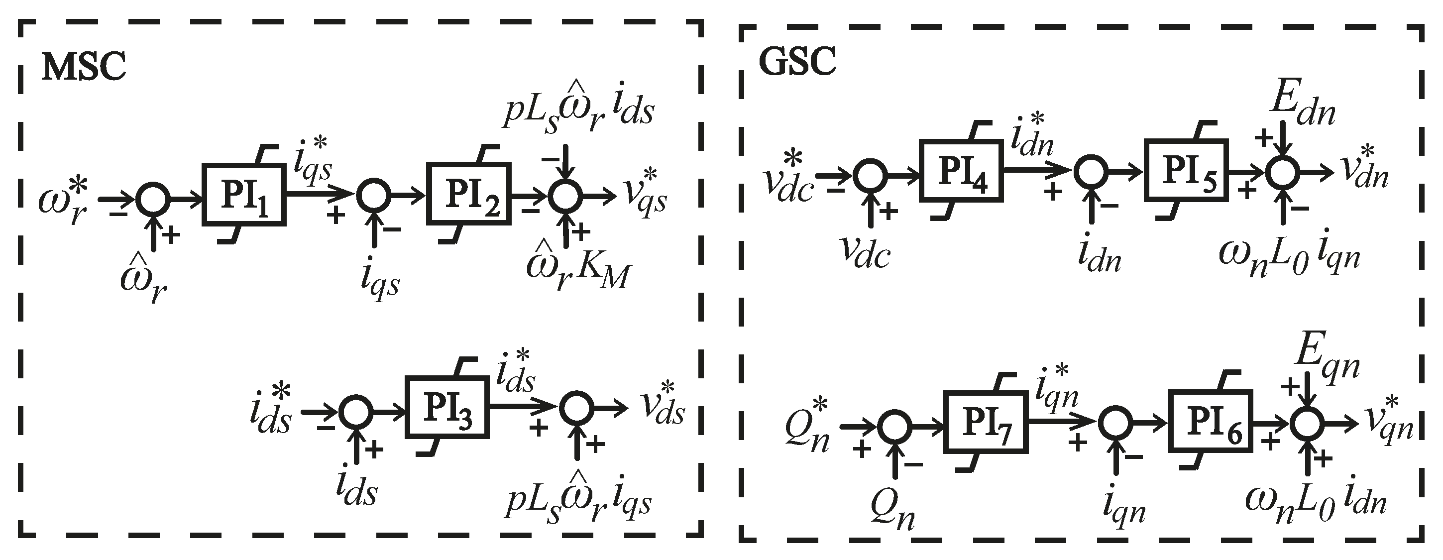
3. Linear Control Scheme for the WTG System

The control loops for the MSC and the GSC using the PI control scheme in a cascaded structure is given in Figure 2. The outer control loops determine the dq axis current reference of each VSC, and the inner control loops regulate the dq axis currents of the MSC and the GSC to the references. The inner loops in Figure 2 are usually designed to be approximately 2–5 times faster than the outer loop to track the references in a suitable time. The PI controllers are tuned considering the stability and performance of the linearized model of the system at the operating points and the desired loop bandwidth. Various on-site PI controller tuning rules are proposed in the literature, e.g., the Cohen–Coon, Ziegler–Nichols, Tyreus–Luyben, Ciancone–Marline, internal model control, and auto-tune methods, with different objectives.

Tuning the PI controller using linear control theory requires a linear plant model. For stability considerations, the real parts of the poles of the plant at the operating point must have negative values. Further, increasing the loop bandwidth enhances the performance and provides a faster response. However, the loop bandwidth and response speed of the plant with a low-order linear controller is limited by control stability considerations. An appropriate gain and phase margin (i.e., typically ${60}^{°}$) of the loop must be considered for adequate stability margins and as a trade-off between the performance and robustness of the plant. Since linear controllers are tuned based on specific operating points, the performance of the linear controller can be affected by the power grid strength at the PCC, e.g., a weak grid, and parameter uncertainty of the WTG.

Next, the analysis of the linearized model of the GSC at the PCC and the influence of a weak grid on linear PI controllers of the GSC are discussed. In a weak grid, the three phase voltages at the PCC are affected by the power flow generated by the WTG. Considering this impact on the linearized model of the feed-forward power control loop (FFPCL) [31], two main stability concerns can be identified, i.e., the existence of an RHP zero and an RHP pole in rectifier and inverter modes of operation, respectively [29,30,31]. The RHP zero and pole are presented briefly next.

Consider the transfer function between the PCC active ($\Delta P_n$) and VSC output voltage ($\Delta v_n$) which is part of the forward path of the FFPCL and is calculated as [31]

$$\begin{gathered} \Delta P_n\approx \frac{1}{\left(L_o+L_n\right)s+R_n}[\left(L_n{\overline{i}}_{dn}s+{\overline{E}}_{dn}\right)\Delta v_n+ \\ \left(L_o{\overline{i}}_{dn}s-{\overline{E}}_{dn}\right)\Delta E_{dg}+\left({\omega }_n\left(L_o+L_n\right){\overline{E}}_{dn}\right)\Delta i_{qn}] \end{gathered}$$

(3)

where $L_n$, $R_n$, ${\overline{i}}_{dn}$, ${\overline{E}}_{dn}$, and $s$ are grid inductance and resistance, the current and voltage of the PCC at the operating point, and the Laplace operator, respectively. As seen in Equation (3), an RHP zero exists in the FFPCL in a rectifier mode of operation (i.e., ${\overline{i}}_{dn}<0$). This RHP zero causes transient undershoot, limits the use of high control gain due to instability, and restricts the closed-loop bandwidth.

Besides, the DC-link-linearized dynamic in the FFPCL is

$$\Delta v_{dc}\approx \frac{{\overline{v}}_{dc}}{Cs{\overline{v}}_{dc}^2-{\overline{P}}_n}\left(-\Delta P_n+{\overline{v}}_{dc}\Delta i_R\right)$$

(4)

where ${\overline{v}}_{dc}$ and ${\overline{P}}_n$ are the DC-link voltage and the PCC active power at the operating point C and $i_R$ are the DC-link capacitance and the output DC current of the MSC shown in Figure 1. Considering the denominator of Equation (4), an RHP exists in the inverter mode of operation (${\overline{P}}_n>0$), which limits the control gain due to instability [31].

Consequently, designing a linear PI controller based on the linearized model of the FFPCL would be insufficient for large variations in the operating point, which is further confirmed through root-locus analysis in [33]. Therefore, a nonlinear control law [42] with global stability will be desirable since it is independent of the operating point and compensates for the variation in operating conditions and grid strength.

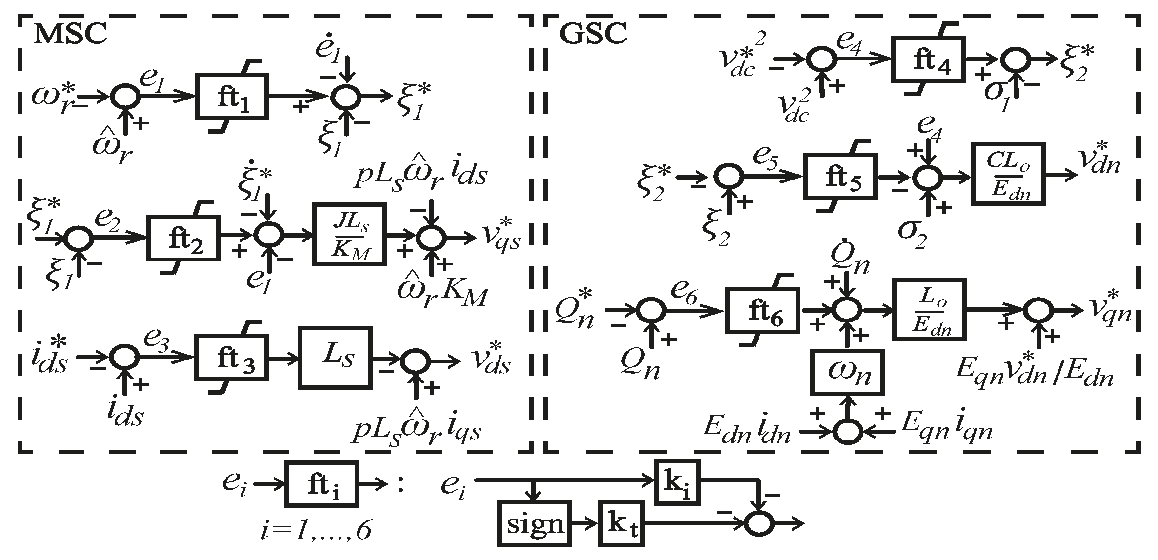
4. Finite-Time Control Design for the PMSG-Based Wind Turbine Generator

In this section, the finite-time stability [41] and back-stepping control design [42] for a nonlinear dynamic system are reviewed first. Then, FTC laws for the MSC and the GSC are designed based on the CLF and back-stepping design techniques.

4.1. FTC and Back-Stepping Control Design

Assume a continuous function $f:D\to {ℝ}^n$ on $D$ containing the origin (i.e., $\mathbf{0}\in D$), and a nonlinear system as

$$\dot{x}=f\left(x\right), f\left(\mathbf{0}\right)=\mathbf{0}, x\in {ℝ}^n$$

(5)

Suppose $V\left(x,t\right):D\to ℝ$ is a Lyapunov function. Then, the origin of Equation (5) is a local finite-time stable equilibrium if

$$\frac{\partial }{\partial t}V+\rho V^{\alpha }\le 0$$

(6)

where $\rho >0$ and $0<\alpha <1$ are real numbers.

Moreover, the origin is a globally finite-time stable equilibrium if $D={ℝ}^n$ and $V$ is radially unbounded. The finite convergence time of the trajectories, i.e., $T\left({\mathbf{x}}_0\right)$, satisfies [34].

$$T\left(x_0\right)\le \frac{V^{1-\alpha }\left(x_0,0\right)}{\rho \left(1-\alpha \right)}$$

(7)

where $x_0=x\left({\mathrm{t}}_0\right)$ is the initial state.

The back-stepping control design technique is often used for a nonlinear system in the form of the following:

$$\{\begin{array}{c}\dot{\mathbf{\chi }}=\mathbf{h}\left(\mathbf{\chi }\right)+\mathbf{g}\left(\mathbf{\chi }\right)\mathbf{\xi } \\ \dot{\mathbf{\xi }}=\mathsf{\nu }\left(\mathbf{\chi }\right)+\mathbf{u}\left(\mathbf{\chi },\mathbf{\xi }\right)\end{array}$$

(8)

where $\mathbf{\chi }=\left[{\mathrm{\chi }}_i\right]$ and $\mathbf{\xi }=\left[{\mathrm{\xi }}_j\right]$ are system state vectors; $u$ is the control vector; and $h$, $g$, and $\mathsf{\nu }$ are smooth vector functions.

The back-stepping design achieves the control of state $\mathbf{\chi }$ through the control of state $\mathbf{\xi }$ since there is no direct control input $u$ available for $\mathbf{\chi }$, as shown in Equation (8). Thus, by controlling $\mathbf{\xi }$, the control input $u$ indirectly controls the state variable $\mathbf{\chi }$ in a back-stepping fashion.

Proposition 1.

Assume that the proposed virtual controller $\mathbf{\xi }={\mathbf{\xi }}_{FT}^{*}\left(\mathbf{\chi }\right)$ is a finite-time stabilizing control law for $\dot{\mathbf{\chi }}$ in Equation (8) and satisfies Equation (6) with a Lyapunov function. Then, the proposed control law (i.e., Equation (9)) stabilizes the origin of the system (i.e., Equation (8)) in finite time:

$${\mathit{u}}_{\mathit{F}\mathit{T}}\left(\mathit{\chi },{\mathit{\xi }}_{\mathit{F}\mathit{T}}^{*}\right)=\frac{\partial {\mathit{\xi }}_{\mathit{F}\mathit{T}}^{*}}{\partial \mathit{\chi }}\left(\mathit{h}+\mathit{g}\mathit{\xi }\right)-\frac{\partial {\mathit{V}}_{\mathit{a}}}{\partial \mathit{\chi }}\mathit{g}-\mathit{k}\left(\mathit{\xi }-{\mathit{\xi }}_{\mathit{F}\mathit{T}}^{*}\right)-\mathit{\nu }-{\mathit{k}}_{\mathit{t}}{\mathit{ℱ}}^{\mathit{\alpha }}\left(\mathit{\xi }-{\mathit{\xi }}_{\mathit{F}\mathit{T}}^{*}\right)$$

(9)

where$\mathit{k}$and${\mathit{k}}_t$are positive real diagonal matrices, i.e.,$\mathit{k}=diag\left(k_i\right)$and${\mathit{k}}_{\mathit{t}}=diag\left(k_{t_i}\right)$, and$ℱ$is the finite-time fractional term proposed as$ℱ\left(\mathit{z}\right)={\left|\mathit{sinh}\left(\mathit{z}\right)\right|}^{\alpha }sign\left(\mathit{z}\right)$,$\mathit{z}\in {ℝ}^n, 0<\alpha <1, \alpha \in ℝ$.

In the proposed controller, ${\mathbf{\xi }}_{FT}^{*}$ is designed as

$${\mathbf{\xi }}_{FT}^{*}\left(\mathbf{\chi }\right)=g^{-1}\left(-h-K\mathbf{\chi }-K_t\mathrm{sign}\left(\mathbf{\chi }\right)\right)$$

Proof. 

First, we show the finite-time stability of system $\dot{\mathbf{\chi }}$ with the proposed controller ${\mathbf{\xi }}_{FT}^{*}\left(\mathbf{\chi }\right)$ and then prove the finite-time stability of the system (i.e., Equation (8)) with the proposed back-stepping controller (i.e., Equation (9)).

The finite-time Lyapunov stability of system $\dot{\mathbf{\chi }}$ can be verified using the candidate control Lyapunov function (CLF). By substituting ${\mathbf{\xi }}_{FT}^{*}\left(\mathbf{\chi }\right)$ to the derivative of the CLF as ${\dot{V}}_a\left(\mathbf{\chi }\right)=\frac{\partial V_a}{\partial \mathbf{\chi }}\dot{\mathbf{\chi }}={\mathbf{\chi }}^T\dot{\mathbf{\chi }}$, we have

$$\begin{array}{cc}{\dot{V}}_a\left(\mathbf{\chi }\right)={\mathbf{\chi }}^T\left(h+g\mathbf{\xi } \right)& ={\mathbf{\chi }}^T\left(-K\mathbf{\chi }-K_t{ℱ}^{\alpha }\left(\mathbf{\chi }\right) \right)\hfill \\ & =-K{\mathbf{\chi }}^T\mathbf{\chi }-K_t{\mathbf{\chi }}^T{\left|\sinh \left(\mathbf{\chi }\right)\right|}^{\alpha }\mathrm{sign}\left(\mathbf{\chi }\right)\hfill \end{array}$$

Considering that $\left|z\right|\le \sinh \left(\left|z\right|\right)\le e^{\left|z\right|}-1$ for $z\in ℝ$, and thus $-{\left|\sinh \left(\mathbf{\chi }\right)\right|}^{\alpha }\le -{\left|\mathbf{\chi }\right|}^{\alpha }$, one concludes

$$\begin{gathered} {\dot{V}}_a\left(\mathbf{\chi }\right)\le -K{\mathbf{\chi }}^T\mathbf{\chi }-K_t\left|{\mathbf{\chi }}^T\right|{\left|\mathbf{\chi }\right|}^{\alpha }\le -{\displaystyle \sum }{k}_i{\mathbf{\chi }}_i^2-{\displaystyle \sum }{k}_{ti}{\left|{\mathbf{\chi }}_i\right|}^{\alpha +1} \\ {\dot{V}}_a\le -2k{V}_a-2^{\beta }{k}_t{V}_a^{\beta } \end{gathered}$$

where $0<\beta =\frac{\alpha +1}{2}<1$ is the fractional power and $k$ and $k_t$ are the minimum eigenvalues of the gain matrices $K$ and $K_t$, respectively. The inequality ${\dot{V}}_a\left(\mathbf{\chi }\right)\le -2^{\beta }{k}_t{V}_a^{\beta }$ shows the finite-time stability of system $\dot{\mathbf{\chi }}$ with the proposed controller ${\mathbf{\xi }}_{FT}^{*}\left(\mathbf{\chi }\right)$ with respect to Equation (7).

Moreover, the finite-time stability of Equation (8) using the proposed controller (Equation (9)) can be proved by using the CLF $V_b=\frac{1}{2}{\left(\mathbf{\xi }-{\mathbf{\xi }}_{FT}^{*}\right)}^T\left(\mathbf{\xi }-{\mathbf{\xi }}_{FT}^{*}\right)$. The detailed proof and derivation of the proposed control laws are given in Appendix A. □

The FTC-based regulators for the MSC and GSC of the WTG are proposed using the back-stepping control design (i.e., Equation (9)). It is noticed that the dynamic equations of ${\omega }_r$ and $v_{dc}^2$ in the WTG model (i.e., Equation (2)) are not directly regulated by any control inputs. Thus, the back-stepping technique is used to design the control law. The q axis current of the MSC and the d axis current of the GSC are used to regulate ${\omega }_r$ and $v_{dc}^2$. Comparing the state space model (i.e., Equation (2)) with Equation (8), we obtain

$$\{\begin{array}{c}\mathbf{\chi }={\left[{\omega }_r,v_{dc}^2\right]}^T\hfill \\ \mathbf{\xi }={\left[-K_M{i}_{qs}/J,-E_{dn}{i}_{dn}/C\right]}^T\hfill \\ \mathbf{u}=\left[-v_{qs}/L_s,-v_{dn}/L_0\right]\hfill \end{array}$$

(10)

4.2. Rotor Speed and Stator Current FTC Design for the MSC

The reference rotor speed ${\omega }_r^{*}$ is determined through the MPPT block in Figure 1. Based on the back-stepping design in Equation (9) and the virtual controller ${\xi }_1=-K_M{i}_{qs}/J$ in Equation (10), the control inputs $v_{qs}^{*}$ and $v_{ds}^{*}$ are proposed as

$${\xi }_1^{*}=\frac{1}{J}\left(F{\omega }_r-T_m\right)+{\dot{\omega }}_r^{*}-k_1{e}_1-k_{t1}\mathrm{sign}\left(e_1\right)$$

(11)

$$v_{qs}^{*}=-\left(r_s{i}_{qs}+L_{s}p{\omega }_r{i}_{ds}-K_M{\omega }_r\right)+\frac{J{L}_s}{K_M}\left({\dot{\xi }}_1^{*}-e_1-k_2{e}_2-k_{t2}{ℱ}^{\alpha }\left(e_2\right)\right)$$

(12)

$$v_{ds}^{*}=L_s\left(k_3{e}_3-\frac{r_s}{L_s}{e}_3+p{\omega }_r{i}_{qs}+k_{t3}{ℱ}^{\alpha }\left(e_3\right)\right)$$

(13)

where $e_1={\omega }_r-{\omega }_r^{*}$, $e_2={\xi }_1-{\xi }_1^{*}$, $e_3=i_{ds}-i_{ds}^{*}$; $k_{ti}$ and $k_i$ are real positive design constants for $i=1, 2, 3$; and ${ℱ}^{\alpha }\left(e_i\right)={\left|\sinh \left(e_i\right)\right|}^{\alpha }\mathrm{sign}\left(e_i\right)$. Moreover, with respect to Equation (11), ${\dot{\xi }}_1^{*}$ is calculated in Appendix A.

The nonlinear control law (Equations (11)–(13)) realizes the ${\omega }_r$ and $i_{ds}$ regulators of the MSC in Figure 1. The detailed derivation of Equations (11)–(13) is given in Appendix A.

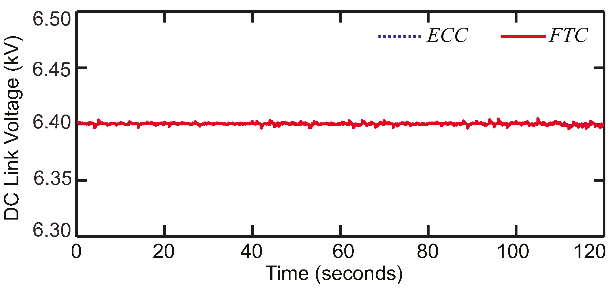
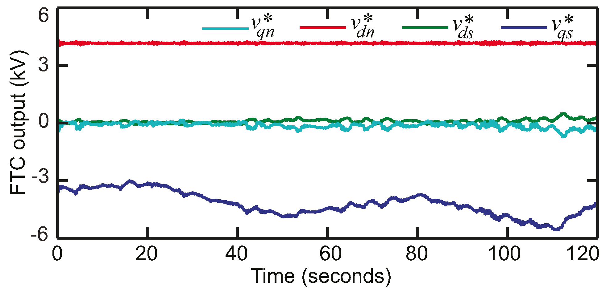
4.3. DC-Link Voltage and Reactive Power FTC for the GSC

The DC-link voltage of the MSC needs to be regulated exactly to its constant reference value ($v_{dc}^{*}$) for stable operation of the WTG. The reactive power injected by the GSC is used to control the PCC voltage. Therefore, the dq currents of the GSC are regulated to achieve the DC voltage and the injected reactive power controls. Based on the back-stepping design in Equation (9) and the virtual controller ${\xi }_2=-E_{dn}{i}_{dn}/C$ in Equation (10), the FTCs $v_{dn}^{*}$ and $v_{qn}^{*}$ are designed as

$${\mathbf{\xi }}_2^{*}=-{\sigma }_1-k_4{e}_4-k_{t4}\mathrm{sign}\left(e_4\right)$$

(14)

$$v_{dn}^{*}=\frac{C{L}_0}{E_{dn}}\left({\sigma }_2+e_4+k_5{e}_5+k_{t5}{ℱ}^{\alpha }\left(e_5\right)\right)$$

(15)

$$v_{qn}^{*}=\frac{L_0}{E_{dn}}\left({\omega }_n{E}_{qn}{i}_{qn}+{\dot{Q}}_n^{*}\right)+{\omega }_n{L}_0{i}_{dn}+\frac{E_{qn}}{E_{dn}}{v}_{dn}^{*}-\frac{L_0}{E_{dn}}\left(k_6{e}_6+k_{t6}{ℱ}^{\alpha }\left(e_6\right)\right)$$

(16)

where $e_4=v_{dc}^2-{\left(v_{dc}^{*}\right)}^2$, $e_5={\xi }_2-{\xi }_2^{*}$, and $e_6=Q_n-Q_n^{*}$. In Equations (14)–(16), $k_t$ and $k_i$ are real positive control design parameters, $s_i=sign\left(e_i\right)$ for $i=4, 5, 6$, and ${\sigma }_1$ and ${\sigma }_2$ are

$${\sigma }_1=-\frac{1}{C}{E}_{qn}{i}_{qn}+\frac{1}{C}{v}_{dc}{i}_R$$

(17)

$${\sigma }_2=k_4{\dot{e}}_4+{\dot{\sigma }}_1+\frac{1}{C{L}_0}{E}_{dn}^2-\frac{1}{C}{\omega }_n{E}_{dn}{i}_{qn}$$

(18)

The nonlinear control law (Equations (14)–(16)) realizes the $v_{dc}$ and $Q$ regulators of the GSC in Figure 1. The detailed derivation of Equations (14)–(16) is not included in the paper for space considerations. It follows a similar derivation procedure as for the MSC. The detailed demonstration of the regulators in Figure 1 for the MSC and the GSC using the proposed nonlinear FTC are depicted in Figure 3. The variables in this diagram are defined in Equations (11)–(16).

4.4. Global Stability Proof of the Proposed FTC for the PMSG

Finite-time stability of the WTG system (Equation (2)) with the proposed FTC is proved using Lyapunov stability criteria. Given the Lyapunov function $V_t=\frac{1}{2}{\displaystyle \sum }_{i=1}^6{e}_i^2$, we have

$${\dot{V}}_t={{\displaystyle \sum }}_{i=1}^6{e}_i{\dot{e}}_i$$

(19)

where $e_i$, $i=1,\dots ,6$ are the errors of the states and have been defined previously. The error dynamics, i.e., ${\dot{e}}_i$, can be calculated using system dynamics (Equation (2)). Substituting the proposed FTC from Equations (11)–(16) into ${\dot{e}}_i$ in Equation (19), we conclude

$${\dot{V}}_t=-{{\displaystyle \sum }}_{i=1}^6{k}_i{e}_i^2-{{\displaystyle \sum }}_{i=1}^6{k}_t{\left|e_i\right|}^{\alpha +1}$$

(20)

Therefore, the WTG system is Lyapunov-stable since ${\dot{V}}_t$ in Equation (20) is negative definite for positive errors.

In addition, considering $-{{\displaystyle \sum }}_{i=1}^6{k}_i{e}_i^2\le 0$ in (20), we have

$${\dot{V}}_t\le -k_t{{\displaystyle \sum }}_{i=1}^6{\left|e_i\right|}^{\alpha +1}\le -2^{\beta }{k}_t{\left(\frac{1}{2}{{\displaystyle \sum }}_{i=1}^6{e}_i^2\right)}^{\beta }$$

(21)

This indicates ${\dot{V}}_t\le -{\rho }_m{V}_t^{\alpha }$ with ${\rho }_m=2^{\beta }{k}_t$ and $\beta =(\alpha +1)/2$, which proves the finite-time stability of Equation (2) with the proposed FTC law (Equations (11)–(16)) in accordance with Equation (6).

If the coefficients $k_t$ of the sign functions are set to zero, the control law (Equations (11)–(16)) becomes the conventional nonlinear exponential convergent controller (ECC) and does not satisfy finite-time convergence in Equation (6) anymore. The comparison of the conventional nonlinear ECC and the proposed FTC is performed in Section 7 for the WTG system.

5. Robustness of and Chattering in the Proposed FTC

Uncertainties due to modeling errors and non-ideal operating conditions are inevitable in practice. Therefore, a robust design of a control system against uncertainties such as parameter variations is important for practical applications. Robustness enhancement of a closed-loop system by the proposed FTC is investigated in this section.

5.1. Robustness against Parameter Uncertainty

To analyze the effect of perturbations on system stability, assume the parameter vector $\mathsf{\theta }$ in Equation (2) as

$$\mathsf{\theta }={\left[J,F,K_M,T_m, r_s, L_s, E_{qn}, E_{dn},C, L_0\right]}^T$$

(22)

An uncertain parameter is formulated as

$${\theta }_j+\mathsf{\Delta }{\theta }_j=\left(1+{\xi }_{\theta j}\right){\theta }_j, 0\le {\xi }_{\theta j}\le 1$$

(23)

where ${\theta }_j$, $\mathsf{\Delta }{\theta }_j={\xi }_{\theta j}{\theta }_j$, and ${\xi }_{\theta j}$ are the nominal parameter, parameter variation, and the uncertainty factor, respectively.

Correspondingly, the dynamics of the perturbed system (Equation (2)) can be separated into a nominal part ($F_N=\left[f_{N_i}\right], i=1\dots 6$) and a perturbed part ($F_{\delta }=\left[f_{{\delta }_i}\right], i=1\dots 6$) as [35]

$${\dot{e}}_i=f_{N_i}\left(t\right)+f_{{\delta }_i}\left(t\right)$$

(24)

It is note that the nominal part is identical to Equation (2), while the perturbed part is a time-variant function of the system states and nominal parameters, i.e., $f_{{\delta }_i}=f_{{\delta }_i}\left(\mathsf{\theta },x,t\right)$.

Suppose the WTG system model (Equation (2)) is perturbed by parameter uncertainties in accordance with Equation (24), the perturbed part $F_{\delta }$ is norm-bounded [42] as

$$\parallel F_{\delta }\parallel \le a+b\parallel e\parallel$$

(25)

where $a$ and $b$ are known real positive constants.

Taking the time derivative of the Lyapunov function $V_t=\frac{1}{2}{\displaystyle \sum }_{i=1}^6{e}_i^2$ for the perturbed system considering Equation (24), we have

$$\frac{\partial V_t}{\partial t}={{\displaystyle \sum }}_{i=1}^6{e}_i{\dot{e}}_i={{\displaystyle \sum }}_{i=1}^6{e}_i\left(f_{N_i}+f_{{\delta }_i}\right)$$

(26)

According to Equation (20), the time derivative of the Lyapunov function $V_t$ for the nominal system can be represented as

$${{\displaystyle \sum }}_{i=1}^6{e}_i{f}_{N_i}=-{{\displaystyle \sum }}_{i=1}^6{k}_i{e}_i^2-{{\displaystyle \sum }}_{i=1}^6{k}_t{\left|e_i\right|}^{\alpha +1}$$

(27)

Substituting Equations (25) and (27) into Equation (26) gives

$$\dot{V}\le {{\displaystyle \sum }}_{i=1}^6\left(-k_i{e}_i^2-k_t{\left|e_i\right|}^{\alpha +1}+e_i\left(a+b\parallel e\parallel \right)\right)$$

(28)

By choosing $k_t\gg a$ and $k_i\gg b$, we obtain

$$\dot{V}\le {{\displaystyle \sum }}_{i=1}^6-\left(k_i-b\right)e_i^2-k_t{\left|e_i\right|}^{\alpha +1}+a{e}_i$$

(29)

which gives $\dot{V}\le 0$ as long as $k_i\ge b$ and $a{e}_i-k_t{\left|e_i\right|}^{\alpha +1}\le 0$. The first inequality constraint can be applied by choosing control gains $k_i$ large enough, $k_i\ge b$; the second inequality constraint is always true for negative errors, $e_i\le 0$. For positive errors, $e_i\ge 0$, the second inequality constraint requires $a\le k_t{e}_i^{\alpha }$. Assume that it is chosen to become robust for a desired range of error, i.e., $\left|e_i\right|\ge c>0$, where $c$ is a real positive constant. Consequently, we must have $a\le k_t{e}_i^{\alpha }$ when ${\left|e_i\right|}^{\alpha }\ge c$, which can be achieved by choosing $k_t$ large enough so that it satisfies $k_t\ge a/c$.

According to Equation (6), Equation (29) indicates the robust stability of the closed-loop system with the proposed FTC with $k_i\ge b$ and $k_t\ge a/c$, for the error range ${\left|e_i\right|}^{\alpha }\ge c$, in the presence of perturbations. In other words, using sufficiently large control gains $k_i$ and $k_t$, the closed-loop system (Equation (2)) with the proposed FTC is robust against the bounded uncertainties. The robustness of the proposed FTC for the WTG system will be verified in Section 7.

5.2. Continuous FTC with Chattering Elimination

The presence of the discontinuous $sign$ function in the FTC (Equations (11)–(16)) leads to a chattering problem and produces undesirable oscillatory control outputs. In this paper, the $sign$ function is approximated using a continuous inverse tangent function to eliminate chattering as

$$sign\left(e\right)\approx \tanh \left(\epsilon e\right)$$

(30)

where $\epsilon \in ℝ$ is a design-specific real constant.

It is noted that increasing the value of $\epsilon$ leads to better approximation of the $sign$ function. However, a very large value of $\epsilon$ may increase the possibility of chattering occurrence. At the same time, $\epsilon$ should be sufficiently large to ensure the robustness of the FTC. When applying the approximation (Equation (30)) in the proposed FTC, the steady-state error of the perturbed system will be bounded (i.e., $\parallel e\parallel \le ϵ, ϵ>0\in ℝ$) [42]. The boundary region $D^{\prime }:\parallel e\parallel \le ϵ$ is determined by the parameter $\epsilon$. The closed-loop trajectories of the perturbed system converge toward and enter the region $D^{\prime }$ in a finite time and will remain inside. An appropriate $\epsilon$ is selected through numerical simulations in this paper.

6. State and Parameter Estimations Using an Adaptive Observer

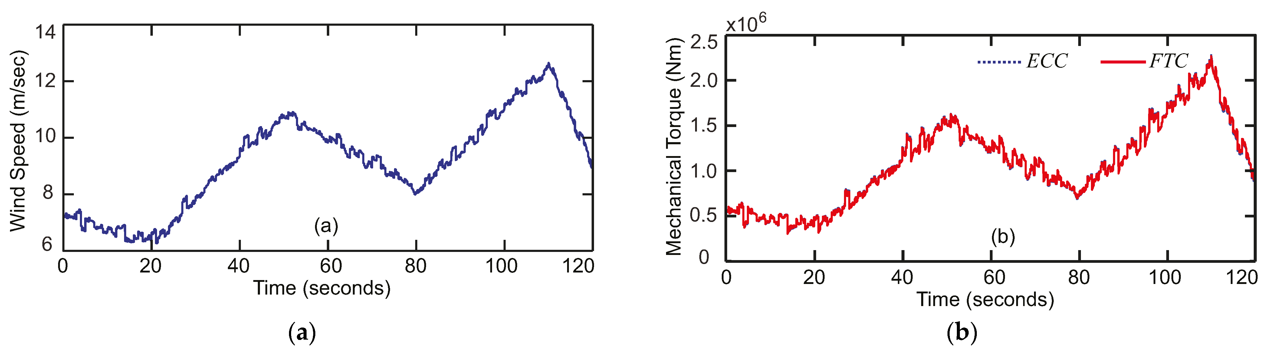
To achieve sensorless control of the PMSG, an adaptive observer [23] is employed to estimate mechanical variables. Since the rotor position is not available, the stationary ($\alpha ,\beta$) reference frame is used for the PMSG model:

$$\{\begin{array}{c}{\dot{x}}_1=A_1{x}_1+B_1+{\left[\begin{array}{cc}0& 1/J\end{array}\right]}^T{T}_m\hfill \\ {\dot{x}}_2=A_2{x}_2+B_2\hfill \end{array}$$

(31)

where the matrices are defined as

$$\{\begin{array}{l}{\mathsf{A}}_1=\left[\begin{array}{cc}-\frac{r_s}{L_s}& p\frac{{\varphi }_{\beta r}}{L_s}\\ \frac{3p{\varphi }_{\beta r}}{2J}& -\frac{F}{J}\end{array}\right],{\mathsf{B}}_1=-\left[\begin{array}{c}\frac{u_{\alpha s}}{L_s}\\ \frac{3p{\varphi }_{\alpha r}{i}_{\beta s}}{2J}\end{array}\right],{\mathsf{x}}_1=\left[\begin{array}{c}{i}_{\alpha s}\\ {\omega }_r\end{array}\right]\\ {\mathsf{A}}_2=-\left[\begin{array}{ccc}\frac{r_s}{L_s}& \frac{p{\omega }_r}{L_s}& 0\\ 0& 0& p{\omega }_r\\ 0& -p{\omega }_r& 0\end{array}\right],{\mathsf{B}}_2=\frac{-1}{L_s}\left[\begin{array}{c}{u}_{\beta s}\\ 0\\ 0\end{array}\right],{\mathsf{x}}_2=\left[\begin{array}{c}{i}_{\beta s}\\ {\varphi }_{\alpha r}\\ {\varphi }_{\beta r}\end{array}\right]\end{array}$$

(32)

In Equation (32), $u_{\alpha s}$, $u_{\beta s}$, $i_{\alpha s}$, $i_{\beta s}$, ${\varphi }_{\alpha r}$, and ${\varphi }_{\beta r}$ are stator voltages, stator currents, and rotor fluxes, respectively, in the stationary reference frame. The adaptive observer and the adaptive law are formulated as Equation (33) and Equation (34), respectively [21]:

$$\{\begin{array}{l}{\dot{\hat{x}}}_1=A_1\left({\hat{x}}_2\right)+B_1\left({\hat{x}}_2\right)+{\left[\begin{array}{cc}0& 1/J\end{array}\right]}^T{\hat{T}}_m\\ \hfill +\lambda {\hat{x}}_1\left[\Gamma {\Gamma }^T/\mu +M_1^{-1}\right]{\left[\begin{array}{cc}{e}_{\alpha i}& 0\end{array}\right]}^T\\ {\dot{\hat{x}}}_2=A_2\left({\hat{\omega }}_r\right){\hat{x}}_2+B_2+M_2^{-1}{\left[\begin{array}{ccc}{e}_{\beta i}& 0& 0\end{array}\right]}^T\end{array}$$

(33)

$$\{\begin{array}{c}{\dot{\hat{T}}}_{\mathrm{m}}={\mathsf{\gamma }}_1\lambda e_{\alpha i}/\mu \hfill \\ \dot{\mu }=-{\eta }_1\mu +{\mathsf{\gamma }}_1^2\hfill \\ \dot{\Gamma }=A_1\Gamma +{\left[\begin{array}{cc}-\lambda {\mathsf{\gamma }}_1{\left(M_1^{-1}\right)}_{1,1}& 1/J\end{array}\right]}^T \hfill \\ {\dot{M}}_1=-{\eta }_0{M}_1-A_1^T\left({\widehat{x}}_2\right)M_1-M_1{A}_1\left({\widehat{x}}_2\right)+\delta {{\rm I}}_2^T{I}_2 \hfill \\ {\dot{M}}_2=-{\eta }_2{M}_2-A_2^T\left({\widehat{\omega }}_r\right)M_2-M_2{A}_2\left({\widehat{\omega }}_r\right)+\delta {{\rm I}}_3^T{I}_3\hfill \end{array}$$

(34)

where ${\eta }_0, {\eta }_1, {\eta }_2, \delta$, and $\lambda$ are real positive constants; $\mu \left(t\right)$ is a time-variable scalar; $M_1$ and $M_2$ are time-variant matrices; ${\left(M_1^{-1}\right)}_{1,1}$ is the (1,1) element of matrix $M_1^{-1}$; $e_{\alpha i}=i_{\alpha s}-{\hat{i}}_{\alpha s}$; $e_{\beta i}=i_{\beta s}-{\hat{i}}_{\beta s}$; $\Gamma ={\left[\begin{array}{cc}{\mathsf{\gamma }}_1& {\mathsf{\gamma }}_2\end{array}\right]}^T$; ${{\rm I}}_2=\left[1,0\right]$; and ${{\rm I}}_3=\left[1,0,0\right]$.

In the dynamic subsystem ${\dot{x}}_1$ of Equation (31), it is desired to estimate the unknown variable $T_m$ and the state vector $x_1$ simultaneously. Therefore, an adaptive Kalman-like observer is used to estimate $x_1$ and $x_2$ by ${\dot{\hat{x}}}_1$ and ${\dot{\hat{x}}}_2$. The stability of the observer can be proved using the Lyapunov function [23]:

$$V_{obs}=e_{o1}^T{M}_{\mathbf{1}}{e}_{o\mathbf{1}}+e_{o\mathbf{2}}^T{M}_{\mathbf{2}}{e}_{o2}+\mu e_{o3}^2$$

(35)

with $e_{o1}=x_{\mathbf{1}}-{\hat{x}}_{\mathbf{1}}-\Gamma e_{o3}$,$e_{o2}=x_{\mathbf{2}}-{\hat{x}}_{\mathbf{2}}$, and $e_{o3}=T_m-{\hat{T}}_m$.

It is assumed that under normal operation of the PMSG wind energy conversion (WEC) system, the data from both wind and torque sensors are used in the proposed controllers rather than the data from the observer. However, the data from the system/parameter observer can be used during sensor failure for a limited period of time, which can improve the reliability of the system. The use of observed data can also be effective if there is a malfunction in the wind and/or torque sensors, such as when the sensor output is out of range. However, although the stability of the observer system is proved by the Lyapunov stability criteria, the delay caused by the observer system has a negative impact on the stability and performance of the system [43], which requires a dedicated investigation.

Applying the chattering elimination in Equation (30) and the adaptive observer in Equation (33), the final output-feedback form of the proposed FTC can be derived from Equations (11)–(16). As an example, the control output $v_{ds}^{*}$ of the proposed FTC is presented as

$$v_{ds}^{*}=L_s\left[k_3{e}_3-\frac{r_s}{L_s}{e}_3+p{\hat{\omega }}_r{i}_{qs}+\frac{2}{\pi }{k}_{t3}{ℱ}^{\alpha }\left(e_3\right)+k_t{\left|\sinh \left(e_3\right)\right|}^{\alpha }\tanh \left(\epsilon e_3\right)\right]$$

(36)

The other control outputs of the FTC in Equations (11)–(16) are not presented due to space considerations.

7. Case Study

A 5MW PMSG-based WTG is simulated using Simulink/SimPowerSystems to verify the proposed FTC and observer algorithms. The WTG parameters are listed in Table 1. Two nonlinear controllers, i.e., the ECC and the FTC, are implemented for the WTG. The ECC is derived by setting $k_t=0$ in the proposed FTC, as described in Section 4. The conventional PI controller is also implemented for the WTG system for benchmark comparison of the control performance to the ECC and FTC. The digital signal processor (DSP) system toolbox is used for the matrix operations of the presented adaptive observer. The initial values of the matrices in Equation (33) are selected as the unity matrix. The parameters of the MSC and GSC of the WTG, the proposed FTC, the adaptive observer, and the PI controller are given in

Table 2. Parameters of the WTG used in the case study.

Quantity	Value
Turbine-rated torque	3.226 × 106 Nm
Rated wind speed	11.8 m/s
PMSG-rated speed	1.55 rad/s
PMSG-rated power	5 MVA

and

Table 3. Parameters of the controllers and the observers.

Quantity	Value
$\mathrm{Control} \mathrm{gains} k_i; i=1\dots 6$	2.7, 9.3 × 103 330, 4, 3.1 × 103, 2.1 × 103
$\mathrm{Finite}-\mathrm{time} \mathrm{gain} k_t$	1
Sign approximation gain $\epsilon$	20
$\mathrm{PI} \mathrm{controller} \mathrm{proportional} \mathrm{gains} k_{P\_i}; i=1\dots 7$	5 × 104, 1.5, 1.5, 5, 1.1, 1.36, 0.01
$\mathrm{PI} \mathrm{controller} \mathrm{integral} \mathrm{gains} k_{I\_i}; i=1\dots 7$	2.5 × 105, 1.2 × 103, 1 × 103, 6 × 102, 8 × 102, 1.2 × 103, 3
Observer adaptive gains ${\eta }_0$, ${\eta }_1$, ${\eta }_2$, $\delta$	1.5 × 104, 2.3 × 104, 1.5 × 104, 1 × 10−6

. Control gains are selected considering the current limits and capacity of the MSC and GSC.

A variant wind profile, illustrated in Figure 4a, is selected for the evaluation of the proposed FTC. The dynamic of the wind profile consists of average value, ramps, gusts, and noise. The mechanical torque of the wind turbine is extracted by the MPPT and rotor speed control and is identical for the FTC and the ECC. The mechanical torque of the wind turbine is shown in Figure 4b.

For the MPPT, the extremum-seeking technique is used since it is independent of the wind turbine’s characteristics. Each harvestable power diagram for a specific wind speed has a peak value, i.e.,$\left({\omega }_r,P_{max}\right)$. Optimum rotor speed reference tracking leads to the MPPT of the WTG. In this paper, a fouth-order polynomial of the stator active power $P_s$ in pu value is used to represent the turbine’s MPPT reference rotor speed as [40,44]

$${\omega }_r^{*}\left(P_s\right)=-2.0768P_s^4+5.6965P_s^3-5.9254P_s^2+3.6040P_s+0.5516$$

(37)

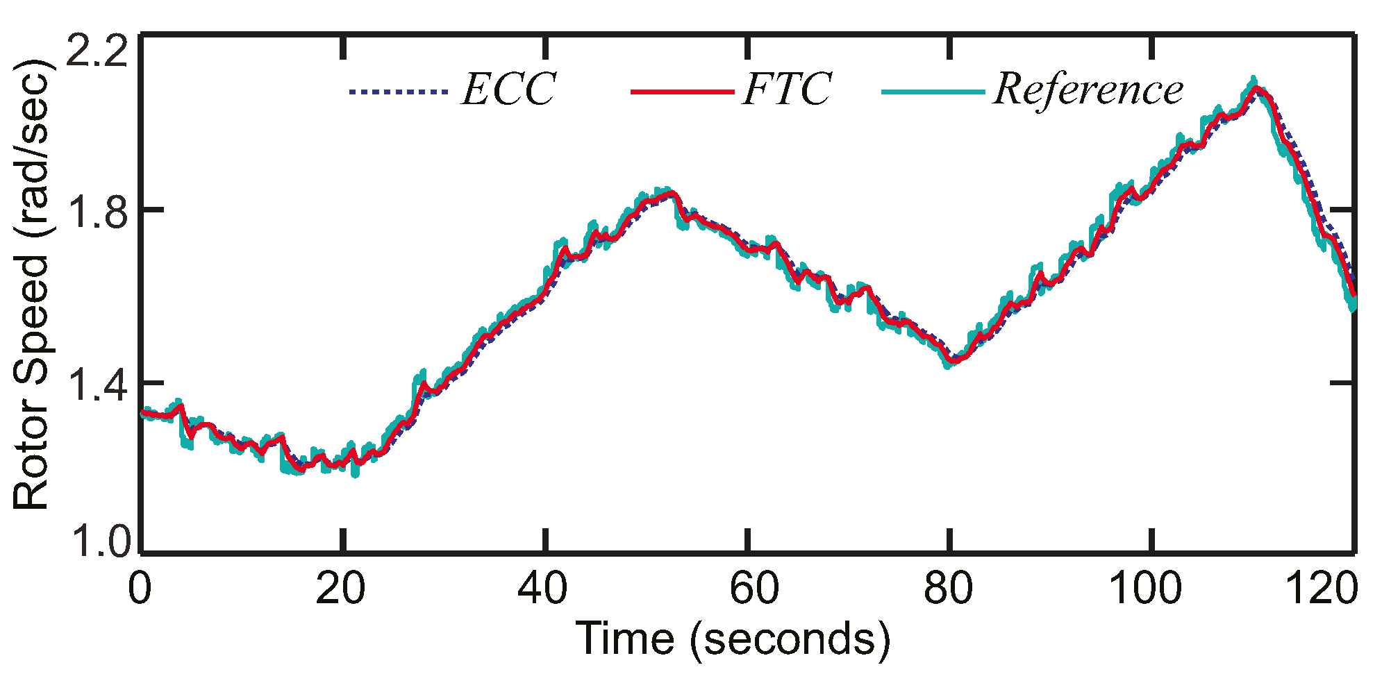
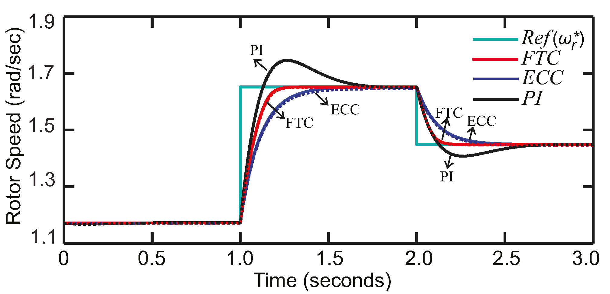
7.1. Rotor Speed Reference Tracking

Figure 5 shows the comparison of the rotor-speed-tracking performance between the proposed FTC and the ECC. The reference rotor speed for the maximum power extraction is determined by the MPPT algorithm. As shown in Figure 5, the FTC provides faster tracking to the reference rotor speed than the ECC does. The average values of the extracted real power using the FTC and the ECC are listed in

Table 4. Mean available and injected active power (MW).

Controller	FTC	ECC	PI Controller
Maximum available		2.091
Measurement based	1.854	1.835	1.817
Observer based	1.846	1.824	1.806

. Two scenarios are compared for different controllers; measurement-based values are calculated using direct rotor speed and WT torque measurements, while observer-based values specify the impact of the adaptive observer transient response. As shown in Table 4, the extracted wind power using the FTC is higher than that using the ECC by 1% since the FTC tracks the optimum rotor speed faster than the ECC does. The relative impact of the transient caused by the adaptive observer on the sensorless MPPT is less than 0.01% compared to the measurement-based MPPT.

To compare the controller outputs of the proposed FTC, the ECC, and the PI controller, an index called control effort (CE) is defined using the mean value of the WTG’s control outputs as

$$CE={\left(\frac{1}{\tau }{{\displaystyle \int }}_0^{\tau }{v}_{ds}^2+v_{qs}^2+v_{dn}^2+v_{qn}^2\right)}^{\frac{1}{2}}$$

(38)

where $\tau$ is the duration of control action.

The average CE for the FTC, the ECC, and the PI controller is 5951, 5948, and 5952, respectively (Figure 5 and Table 4). The proposed FTC extracts more power compared to the ECC and the PI controller though using an identical CE, which relatively differs only by 0.05%.

Figure 6 shows the unextracted wind powers by the FTC and the ECC when the adaptive observer is used. As shown in Figure 6, the FTC presents a smaller unextracted wind power compared to the ECC and improves the MPPT algorithm by accurate and fast tracking of the reference rotor speed.

The GSC of the WTG regulates a constant DC-link voltage under the condition of varying wind power output, as depicted in Figure 7. The reactive power reference of the GSC regulates a unity power factor at the PCC. As shown in Figure 7, the DC-link voltage is effectively regulated by the FTC and the ECC under fluctuating wind power. Figure 8 illustrates the control outputs of the proposed FTC for the case study. It is observed in Figure 8 that the control signals are in the practical range without chattering and saturation.

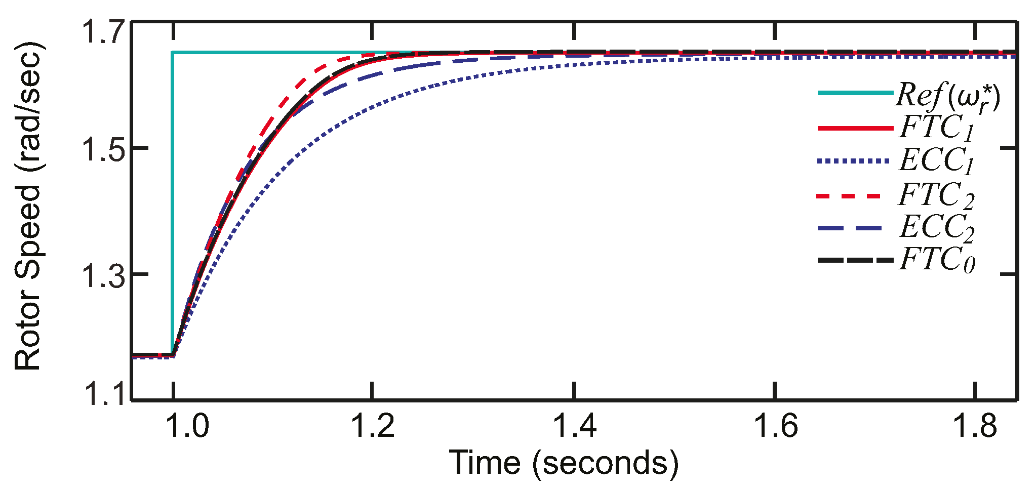
7.2. Robustness of the Proposed Nonlinear Controls against Uncertainties

The robustness of the closed-loop WTG system using the proposed FTC is investigated under the perturbed condition in which the magnitudes of the WTG parameters increase by 20% from the nominal values. The performance of the proposed FTC is compared to the ECC and the PI controller under nominal and perturbed conditions (Figure 9).

CE values are calculated for the FTC, the ECC, and the PI controller under nominal and perturbed conditions. Figure 10 illustrates that the control effort of the proposed FTC is analogous to the ECC and the PI controller. The proposed FTC provides lower overshoot compared to the PI controller and the ECC, although it uses a similar average CE. Therefore, the FTC is robust against uncertainty and improves the transient response under the perturbed condition as well as the nominal condition. In addition, the Bode diagram of the PI controller’s outer control loops for rotor speed and DC-link voltage in Figure 11 illustrates appropriate tuning of the PI controller with high and sufficient stability margins and robustness.

As discussed in Section 4, the robustness of the proposal FTC is influenced by the control gains $k_i$ and $k_t$. Three scenarios are created to analyze the impact of control gains. First, the response of the nominal WTG is evaluated for the FTC with nominal control gains given in Table 3. The simulated rotor speed response is denoted as FTC0 in Figure 12. Second, the same control gains $k_i$ and $k_t$ in Table 3 are used by the FTC and the ECC for the perturbed system. The resultant responses are denoted as FTC1 and ECC1 in Figure 12. Third, the control gains $k_i$ and $k_t$ for the FTC and the ECC are multiplied by a factor of 1.5 and denoted by FTC2 and ECC2. As depicted in Figure 12, the settling time and the steady-state error of the rotor speed are reduced by increasing the control gains $k_i$ and the finite-time gain $k_t$ under the perturbed condition. It is also shown in Figure 12 that the steady-state error and the settling time of the response with the proposed FTC are lower than the ECC’s. The relative tracking error by the proposed FTC is 0.12% for the perturbed system and is zero for the nominal system.

In Figure 13, the impact of increasing the control gains $k_i$ and $k_t$ on the settling time and the steady-state error of the closed-loop WTG’s response is illustrated for the perturbed system. For the label, FTC $k_i$ inc., used in Figure 13, the FTC’s gain $k_i$ increases from 1 to 1.5 and 2 pu, while $k_t$ is kept constant at 1 pu. Other labels in Figure 13 follow the similar notation as FTC $k_i$ inc. It is observed in Figure 13 that the FTC presents a shorter settling time and a smaller steady-state error compared to the ECC for various control gains $k_t$ and $k_i$.

7.3. Implemmention of the Adaptive Observer

The implementation of the adaptive observer proposed in Section 5 is investigated for the FTC in this section. The estimation of the mechanical variables ${\omega }_r$ and $T_m$ by the adaptive observer are shown in Figure 14 for the step change in wind speed. The results illustrate that the proposed observer accurately tracks the reference rotor speed and the mechanical torque in the steady state. As depicted in Figure 14b, the mechanical torque $T_m$ estimation has been designed to have a slower transient response in order to suppress any measurement noise presented in $T_m$. The proposed adaptive observer generates an accurate estimation of $T_m$ in the steady state, which is essential for the controller stability. It is noted that the estimation error may lead to a minor loss of MPPT during the transient response of the observation.

7.4. Performance of the GSC FTC for a Weak Grid

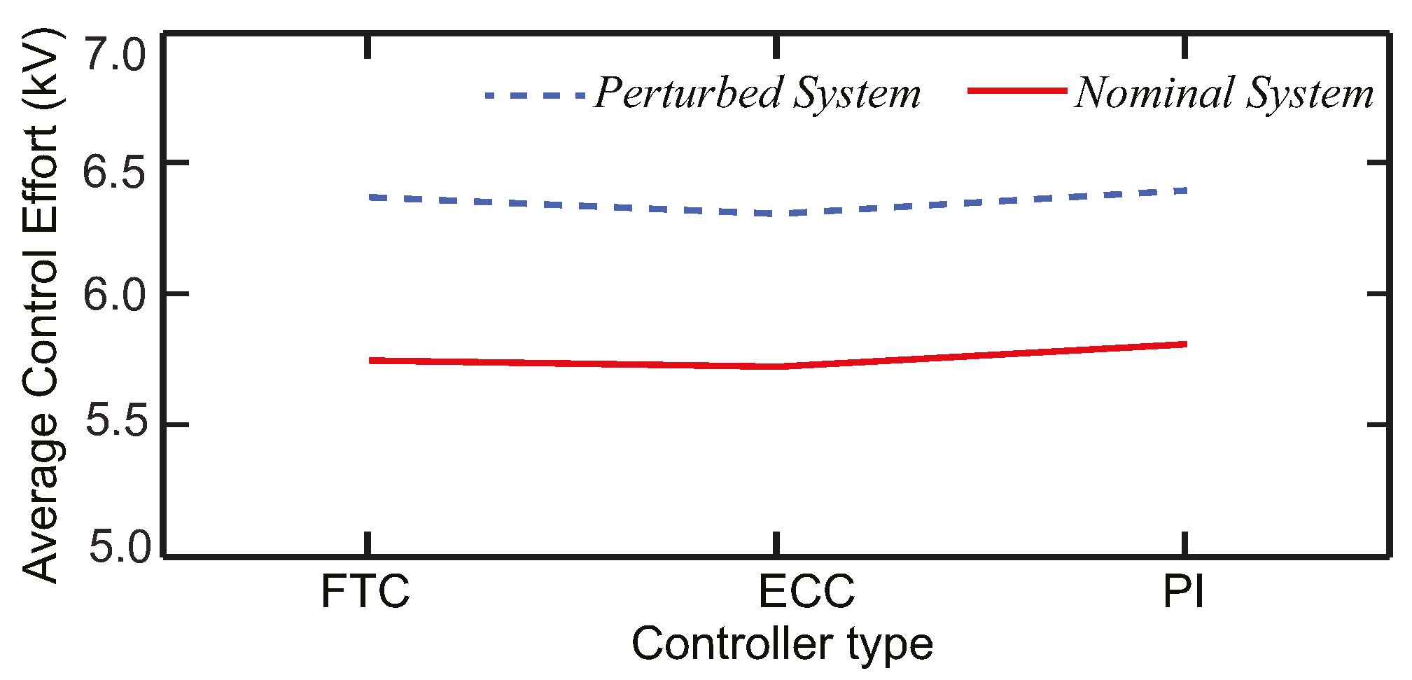
The robustness of the proposed FTC, ECC, and PI controller was analyzed in Section 5. In this subsection, the impact of the different grid strength and injected reactive power on the variations in the PCC’s voltage is investigated. A step change is applied to the wind speed, which is identical to Figure 9. The performance and resiliency of the proposed FTC are compared to the PI controller for the GSC of the WTG connecting to a weak grid in Figure 15a and Figure 15b, respectively. Commonly, a grid with an SCR lower than 20 is considered a weak grid. Furthermore, the impact of the PCC reactive power control (or GSC q axis current control) is depicted in Figure 15 for a grid with SCRs 5 and 19.

When a step change in the active power of the MSC occurs, the power has to be injected into the grid through the GSC in order to regulate a constant DC-link voltage. Moreover, enabling the reactive power control at the PCC compensates the steady-state PCC voltage variation caused by the grid strength. The DC-link voltage and PCC reactive power are regulated using the GSC d and q axis currents, respectively.

The proposed PI controller is also effective for the weak power grid.

As demonstrated in Figure 15, the steady-state variation and the transient overshoot in the PCC’s voltage magnitude are lower with the proposed FTC (Figure 15a) compared to the conventional PI controller (Figure 15b) since the FTC provides an advanced transient in the GSC dq axis currents and eliminates overshoot.

Similar to the uncompensated case, the proposed FTC (Figure 15a) further improves the transient in the PCC’s voltage magnitude compared to the conventional PI controller (Figure 15b) when the PCC reactive power control is enabled (i.e., $Q_n^{*}\ne 0$), as well as with unity power factor (i.e., $Q_n^{*}=0$).

7.5. Discussion

The proposed FTC is developed based on the existing ECC [40] with minor modifications, i.e., adding a finite-time term to each dynamic of the control errors. It is a critical variation, as the system can move from an FTC to an ECC and vice versa easily, yet take the advantages of finite-time convergence. The performance of the proposed FTC is compared to the ECC proposed in [40] and the conventional PI control method. Although the performance of the proposed nonlinear FTC is comparable to nonlinear high-order sliding mode control, the proposed FTC has the advantage that it can be easily implemented by slightly modifying the conventional ECC, i.e., by adding finite-time terms with a fractional power. Since the proposed FTC is developed by adding simple terms to the conventional ECC, its implementation in practice should have the same level of difficulties.

8. Conclusions

This paper proposed a finite-time nonlinear controller for the PMSG-based WTG system. The nonlinear controls of the machine-side converter and the grid-side converter are based on the control Lyapunov function and back-stepping control design techniques. Rotor speed and current are regulated through the machine-side converter for MPPT, whereas the voltage of the DC link is controlled using the grid-side converter’s current regulators. The robustness of the proposed controller was studied for bounded uncertainties. The proposed multi-loop output-feedback nonlinear FTC improves the control robustness against a bounded uncertainty, such as parameter variations, only by the proper tuning of its control gains, as the most effective part in the proposed scheme responsible for robustness against parameter uncertainties. Minimum required control gains to provide robustness against bounded uncertainties are calculated based on the Lyapunov stability theorem. A 5MW WTG is used in the case study to verify the effectiveness of the proposed nonlinear finite-time control techniques. The performance of the proposed FTC is compared with the ECC and the PI controller for the WTG under nominal and perturbed conditions. Simulation studies verify that the proposed FTC achieves fast and accurate MPPT and improves the controller robustness for parameter uncertainties and for a weak power grid compared to the conventional ECC and PI controllers. It also enhances stability of the system. The robustness of the proposed FTC is verified using aperturbed WTG system with 20% parameter variation and a weak power grid at the PCC. Moreover, the outer reactive power control loop is used to control the AC voltage in a weak grid at the PCC with a low circuit ratio. In a weak grid, the proposed FTC improves the steady-state variation and the transient overshoot in the PCC’s voltage compared to the conventional PI controller. As future research work, the authors aim to address the impacts of the delay caused by the observer on the performance and stability of the PMSG WEC system with different control methods, using the Lyapunov–Krasovskii linear matrix inequality (LMI) method for time delay systems.

References

1. Chinchilla, M.; Arnaltes, S.; Burgos, J.C. Control of permanent-magnet generators applied to variable-speed wind-energy systems connected to the grid. IEEE Trans. Energy Convers. 2006, 21, 130–135. [Google Scholar] [CrossRef] [Green Version]
2. Xia, Y.; Ahmed, K.H.; Williams, B.W. Wind turbine power coefficient analysis of a new maximum power point tracking technique. IEEE Trans. Ind. Electron. 2013, 60, 1122–1132. [Google Scholar] [CrossRef]
3. Yang, X.; Gong, X.; Qiao, W. Mechanical sensorless maximum power tracking control for direct-drive PMSG wind turbines. In Proceedings of the 2010 IEEE Energy Conversion Congress and Exposition (ECCE), Atlanta, GA, USA, 12–16 September 2010. [Google Scholar]
4. Rocha, R. A sensorless control for a variable speed wind turbine operating at partial load. Renew. Energy 2011, 36, 132–141. [Google Scholar] [CrossRef] [Green Version]
5. Tan, K.; Islam, S. Optimum control strategies in energy conversion of PMSG wind turbine system without mechanical sensors. IEEE Trans. Energy Convers. 2008, 19, 392–399. [Google Scholar] [CrossRef]
6. Blaabjerg, F.; Chen, Z.; Kjaer, S.B. Power electronics as efficient interface in dispersed power generation systems. IEEE Trans. Power Electron. 2004, 19, 1184–1194. [Google Scholar] [CrossRef]
7. Rigatos, G.; Siano, P.; Zervos, N. Sensorless control of distributed power generators with the derivative-free nonlinear Kalman filter. IEEE Trans. Ind. Electron. 2014, 61, 6369–6382. [Google Scholar] [CrossRef]
8. Pourebrahim, R.; Tohidi, S.; Younesi, A. Sensorless model adaptive control of DFIG by using High frequency signal injection and fuzzy logic control. Iran. J. Electr. Electron. Eng. 2018, 14, 11–21. [Google Scholar]
9. Qiao, W.; Zhou, W.; Aller, J.M.; Harley, R.G. Wind Speed Estimation Based Sensorless Output Maximization Control for a Wind Turbine Driving a DFIG. IEEE Trans. Power Electron. 2008, 23, 1156–1169. [Google Scholar] [CrossRef]
10. Qiao, W.; Harley, R.G.; Venayagamoorthy, G.K. Coordinated Reactive Power Control of a Large Wind Farm and a STATCOM Using Heuristic Dynamic Programming. IEEE Trans. Energy Convers. 2009, 24, 493–503. [Google Scholar] [CrossRef] [Green Version]
11. Fatu, M.; Blaabjerg, F.; Boldea, I. Grid to standalone transition motion-sensorless dual-inverter control of PMSG with asymmetrical grid voltage sags and harmonics filtering. IEEE Trans. Power Electron. 2014, 29, 3463–3472. [Google Scholar] [CrossRef]
12. Song, X.; Fang, J.; Han, B.; Zheng, S. Adaptive Compensation Method for High-Speed Surface PMSM Sensorless Drives of EMF-Based Position Estimation Error. IEEE Trans. Power Electron. 2016, 31, 1438–1449. [Google Scholar] [CrossRef]
13. Abdelrahem, M.; Hackl, C.M.; Kennel, R. Finite Position Set-Phase Locked Loop for Sensorless Control of Direct-Driven Permanent-Magnet Synchronous Generators. IEEE Trans. Power Electron. 2018, 33, 3097–3105. [Google Scholar] [CrossRef]
14. Abdelrahem, M.; Hackl, C.M.; Kenne, R.; Rodríguez, J. Computationally Efficient Finite-Position-Set-Phase-Locked Loop for Sensorless Control of PMSGs in Wind Turbine Applications. IEEE Trans. Power Electron. 2021, 36, 3007–3016. [Google Scholar] [CrossRef]
15. Ali, M.A.S.; Mehmood, K.K.; Baloch, S.; Kim, C. Wind-Speed Estimation and Sensorless Control for SPMSG-Based WECS Using LMI-Based SMC. IEEE Access 2020, 8, 26524–26535. [Google Scholar] [CrossRef]
16. Liang, D.; Li, J.; Qu, R.; Kong, W. Adaptive Second-Order Sliding-Mode Observer for PMSM Sensorless Control Considering VSI Nonlinearity. IEEE Trans. Power Electron. 2018, 33, 8994–9004. [Google Scholar] [CrossRef]
17. Wang, Y.; Xu, Y.; Zou, J. Sliding-Mode Sensorless Control of PMSM with Inverter Nonlinearity Compensation. IEEE Trans. Power Electron. 2019, 34, 10206–10220. [Google Scholar] [CrossRef]
18. Pan, Y.; Yang, C.; Pan, L.; Yu, H. Integral Sliding Mode Control: Performance, Modification, and Improvement. IEEE Trans. Ind. Inform. 2018, 14, 3087–3096. [Google Scholar] [CrossRef]
19. Zhang, Z.; Zhao, Y.; Qiao, W.; Qu, L. A space-vector-modulated sensorless direct-torque control for direct-drive PMSG wind turbines. IEEE Trans. Ind. Appl. 2014, 50, 2331–2341. [Google Scholar] [CrossRef]
20. Yan, J.; Lin, H.; Feng, Y.; Guo, X.; Huang, Y.; Zhu, Z.Q. Improved sliding mode model reference adaptive system speed observer for fuzzy control of direct-drive permanent magnet synchronous generator wind power generation system. IET Renew. Power Gener. 2013, 7, 28–35. [Google Scholar] [CrossRef]
21. Beltran, B.; Benbouzid, M.E.H.; Ahmed-Ali, T. Second-Order Sliding Mode Control of a Doubly Fed Induction Generator Driven Wind Turbine. IEEE Trans. Energy Convers. 2012, 27, 261–269. [Google Scholar] [CrossRef] [Green Version]
22. Benbouzid, M.E.H.; Beltran, B.; Amirat, Y.; Yao, G.; Han, J. Second-Order Sliding Mode Control for DFIG-Based Wind Turbines Fault Ride-Through Capability Enhancement. ISA Trans. 2014, 53, 827–833. [Google Scholar] [CrossRef] [PubMed] [Green Version]
23. Besancon, G.; Leon-Morales, J.D.; Huerta-Guevara, O. On adaptive observers for state affine systems. Int. J. Control 2006, 79, 581–591. [Google Scholar] [CrossRef]
24. Haque, M.E.; Negnevitsky, M.; Muttaqi, K.M. A novel control strategy for a variable-speed wind turbine with a permanent-magnet synchronous generator. IEEE Trans. Ind. Appl. 2010, 46, 331–339. [Google Scholar] [CrossRef] [Green Version]
25. Geng, H.; Xu, D. Stability analysis and improvements for variable-speed multipole permanent magnet synchronous generator-based wind energy conversion system. IEEE Trans. Sustain. Energy 2011, 2, 459–467. [Google Scholar] [CrossRef]
26. Geng, H.; Yang, G.; Xu, D.; Wu, B. Unified Power Control for PMSG-Based WECS Operating Under Different Grid Conditions. IEEE Trans. Energy Convers. 2011, 26, 822–830. [Google Scholar] [CrossRef]
27. Debnath, S.; Saeedifard, M. A new hybrid modular multilevel converter for grid connection of large wind turbines. IEEE Trans. Sustain. Energy 2013, 4, 1051–1064. [Google Scholar] [CrossRef]
28. Li, S.; Haskew, T.A.; Xu, L. Conventional and novel control designs for direct driven PMSG wind turbines. Electr. Power Syst. Res. 2010, 80, 328–338. [Google Scholar] [CrossRef]
29. Giraldo, E.; Garces, A. An adaptive control strategy for a wind energy conversion system based on PWM-CSC and PMSG. IEEE Trans. Power Syst. 2014, 29, 1446–1453. [Google Scholar] [CrossRef]
30. Muljadi, E.; Butterfield, C.P.; Parsons, B.; Ellis, A. Effect of variable speed wind turbine generator on stability of a weak grid. IEEE Trans. Energy Convers. 2007, 22, 29–36. [Google Scholar] [CrossRef]
31. Wang, W.; Beddard, A.; Barnes, M.; Marjanovic, O. Analysis of active power control for VSC–HVDC. IEEE Trans. Power Deliv. 2014, 29, 1978–1988. [Google Scholar] [CrossRef]
32. Yuan, X.; Wang, F.; Boroyevich, D.; Li, Y.; Burgos, R. DC-link voltage control of a full power converter for wind generator operating in weak-grid systems. IEEE Trans. Power Electron. 2009, 24, 2178–2192. [Google Scholar] [CrossRef]
33. Strachan, N.P.W.; Jovcic, D. Stability of a variable-speed permanent magnet wind generator with weak AC grids. IEEE Transactions on Power Delivery 2010, 25, 2779–2788. [Google Scholar] [CrossRef]
34. Xi, X.; Geng, H.; Yang, G. Enhanced model of the doubly fed induction generator-based wind farm for small-signal stability studies of weak power system. IET Renew. Power Gener. 2014, 8, 765–774. [Google Scholar] [CrossRef]
35. Mitra, P.; Zhang, L.; Harnefors, L. Offshore wind integration to a weak grid by VSC-HVDC links using power-synchronization control: A case study. IEEE Trans. Power Deliv. 2014, 29, 453–461. [Google Scholar] [CrossRef]
36. Neris, A.S.; Vovos, N.A.; Giannakopoulos, G.B. A variable speed wind energy conversion scheme for connection to weak AC systems. IEEE Trans. Energy Convers. 1999, 14, 122–127. [Google Scholar] [CrossRef]
37. Lin, W.M.; Hong, C.M.; Lee, M.R.; Huang, C.H.; Huang, C.C.; Wu, B.L. Fuzzy sliding mode-based control for PMSG maximum wind energy capture with compensated pitch angle. In Proceedings of the 2010 International Symposium on Computer, Communication, Control and Automation (3CA), Tainan, Taiwan, 5–7 May 2010; pp. 397–400. [Google Scholar]
38. Lin, W.M.; Hong, C.M.; Chen, C.H. Neural-network-based MPPT control of a stand-alone hybrid power generation system. IEEE Trans. Power Electron. 2011, 26, 3571–3581. [Google Scholar] [CrossRef]
39. Koutiva, X.I.; Vrionis, T.D.; Vovos, N.A.; Giannakopoulos, G.B. Optimal integration of an offshore wind farm to a weak AC grid. IEEE Trans. Power Deliv. 2006, 21, 987–994. [Google Scholar] [CrossRef]
40. Magri, A.E.; Giri, F.; Besancon, G.; Fadili, A.E.; Dugard, L.; Chaoui, F.Z. Sensorless adaptive output feedback control of wind energy systems with PMS generators. Control Eng. Pract. 2013, 21, 530–543. [Google Scholar] [CrossRef] [Green Version]
41. Shotorbani, A.M.; Mohammadi, B.; Wang, L.; Marzband, M.; Sabahi, M. Application of finite-time control Lyapunov function in low-power PMSG wind energy conversion systems for sensorless MPPT. Electr. Power Energy Syst. 2019, 106, 169–182. [Google Scholar] [CrossRef]
42. Khalil, H.K. Nonlinear Systems, 3rd ed.; Prentice Hall: Upper Saddle River, NJ, USA, 2011. [Google Scholar]
43. Sami, I.; Ullah, S.; Ullah, N.; Ro, J.S. Sensorless fractional order composite sliding mode control design for wind generation system. ISA Trans. 2020. [Google Scholar] [CrossRef] [PubMed]
44. Gonzales, L.G.; Figueres, E.; Garcera, G.; Carranza, O. Maximum-power-point tracking with reduced mechanical stress applied to wind-energy-conversion-systems. Appl. Energy 2010, 87, 2304–2312. [Google Scholar] [CrossRef] [Green Version]
Figure 1. Permanent magnet synchronous generator (PMSG)-based wind energy conversion system.
Energies 14 01712 g001
Figure 2. PI control scheme for comparison with the proposed finite-time controller (FTC).
Energies 14 01712 g002
Figure 3. Block diagram of the proposed FTC.
Energies 14 01712 g003
Figure 4. Input and output of the wind turbine: (a) wind speed profile and (b) mechanical output torque of the wind turbine.
Energies 14 01712 g004
Figure 5. Rotor speed tracking by the ECC and the FTC.
Energies 14 01712 g005
Figure 6. The unextracted wind power due to the transients in reference tracking of the FTC and the ECC.
Energies 14 01712 g006
Figure 7. DC-link voltage.
Energies 14 01712 g007
Figure 8. Reference control outputs of the MSC and the GSC by the FTC.
Energies 14 01712 g008
Figure 9. Comparison of the proposed FTC to the ECC and the PI controller: rotor speed reference-tracking performance.
Energies 14 01712 g009
Figure 10. Average control efforts of the FTC, the ECC, and the PI controller for nominal and perturbed systems.
Energies 14 01712 g010
Figure 11. Bode diagram of the closed-loop WTG system with the proposed PI controller.
Energies 14 01712 g011
Figure 12. Responses of FTCs and ECCs under nominal and perturbed conditions.
Energies 14 01712 g012
Figure 13. Effects of an increase in k i and k t on responses of the perturbed WTG with the FTC and ECC: (a) settling time and (b) relative steady-state error.
Energies 14 01712 g013
Figure 14. Mechanical output from the adaptive observer: (a) rotor speed ω r and (b) mechanical torque T m .
Energies 14 01712 g014
Figure 15. Impact of the grid strength on the PCC voltage magnitude with different controllers: (a) proposed FTC and (b) conventional PI controller.
Energies 14 01712 g015