Article

Analysis of Aeroacoustic Properties of the Local Radial Point Interpolation Cumulant Lattice Boltzmann Method

1
Department of Mechanical Engineering, ETSEQ, Rovira i Virgili University, Països Catalans, 26, 43007 Tarragona, Spain
2
Department of Mechanical Engineering, The University of Manchester, Oxford Rd, Manchester M13 9PL, UK
*
Author to whom correspondence should be addressed.
Energies 2021, 14(5), 1443; https://doi.org/10.3390/en14051443
Submission received: 11 January 2021 / Revised: 26 February 2021 / Accepted: 2 March 2021 / Published: 6 March 2021
(This article belongs to the Special Issue The Numerical Simulation of Fluid Flow)

Abstract

:
The lattice Boltzmann method (LBM) has recently been used to simulate wave propagation, one of the challenging aspects of wind turbine modeling and simulation. However, standard LB methods suffer from the instability that occurs at low viscosities and from its characteristic lattice uniformity, which results in issues of accuracy and computational efficiency following mesh refinement. The local radial point interpolation cumulant lattice Boltzmann method (LRPIC-LBM) is proposed in this paper to overcome these shortcomings. The LB equation is divided into collision and streaming steps. The collision step is modeled by the cumulant method, one of the stable LB methods at low viscosities. In addition, the streaming step, which is naturally a pure advection equation, is discretized in time and space using the Lax–Wendroff scheme and the local radial point interpolation method (RPIM), a mesh free method. We describe the propagation of planar acoustic waves, including the temporal decay of a standing plane wave and the spatial decay of a planar acoustic pulse. The analysis of these specific benchmark problems has yielded qualitative and quantitative data on acoustic dispersion and dissipation, and their deviation from analytical results demonstrates the accuracy of the method. We found that the LRPIC-LBM replicates the analytical results for different viscosities, and the errors of the fundamental acoustic properties are negligible, even for quite low resolutions. Thus, this method may constitute a useful platform for effectively predicting complex engineering problems such as wind turbine simulations, without parameter dependencies such as the number of points per wavelength N p p w and resolution σ or the detrimental effect caused by the use of coarse grids found in other accurate and stable LB models.

1. Introduction

Evidence of early sailing boats on the Nile and of Persian pumps and mills from the first century B.C. shows humans have been interested in Wind Energy since ancient times [1]. In general, a wind turbine is defined as a device which converts the wind’s kinetic energy into electrical energy [2,3]. It plays a key role on producing intermittent renewable energy and implementing a strategy to lower costs and reducing the reliance on fossil fuels [4,5]. Wind turbines have unique aerodynamic and aeroacoustic behavior that makes their prediction most challenging [6,7], particularly their simulation needs an enormous number of grid points or cells, and long enough time samples [8]. Researchers and centers such as the National Renewable Energy Laboratory (NREL) and the National Wind Technology Center (NWTC) have initiated multi-year programs on aeroacoustic wind turbine modeling [9] to develop efficient and appropriate computational aeroacoustic (CAA) implementations. Among particular issues specified to wind turbine problems, the propagation of sound is always a significant computational challenge [10,11]. With this aim, different numerical approaches were developed in the field of computational aeroacoustics. Tam [12] and Wells et al. [13] proposed popular numerical schemes such as compact and non-compact optimized schemes like the high-order compact difference scheme [14] and the dispersion-relation-preserving (DRP) scheme [15]. Cheong et al. proposed grid-optimized dispersion-relation-preserving (GODRP) schemes for aeroacoustic simulations [16]. Due to the huge cost of CAA simulations, hybrid methods using two sets of equations, one for the flow and another one for the acoustic disturbance field were developed [17].
Direct aerostatic simulations are computer-intensive due to the small ratio between sound pressure and pressure variation as a whole, the spreading of acoustic fields over a large area, and the time-consuming nature of traditional methods [18]. As an illustration, the direct numerical simulation of waves using Navier–Stokes equations requires schemes of fifth-order accuracy in space and fourth order accuracy in time [19,20]. Therefore, the lattice Boltzmann method (LBM), an explicit time marching scheme [21], has been widely used as an alternative to simulate sound wave propagation due to its kinetic nature, relative simplicity of implementation and parallelization. The LBM as a mesoscopic method uses probability density functions (probability of finding particles within a certain range of velocities at a certain range of locations at a given time) to model the momentum distribution in discrete space, thereby economizing computer resources [22]. Buick et al. [23] and Dellar et al. [24] studied sound wave propagation using LBM and achieved acceptable results. Bres et al. [25] and Gorakifard et al. [26] presented the dissipation and dispersion of acoustic waves using the BGK-LBM and the cumulant LBM, respectively. Furthermore, a regularized method for the BGK-LBM [27] and the recursive and regularized LBM (LBM-rrBGK) [28,29] have been developed to model wave propagation.
One of the drawbacks of the LBM is lattice uniformity, originated from symmetric lattice velocity models such as the square and cubic lattice meshes in 2D/3D simulations [30]. Lattice uniformity causes the streaming step to occur at uniform neighboring grid points. Thus, the LBM is only applied to uniform meshes, whereas issues of accuracy and computational efficiency mainly affect simulations of problems that require non-uniform meshes. For example, numerical simulations with curved and irregular boundaries, common in wind turbine simulations, encounter difficulties when fitting the grids to the boundaries or adapting complex computational domains. Grid refinement schemes or adaptive LBM can help to simulate curved and moving boundaries more accurately [31]. Wood [32] used refinement in LBM simulations to analyze wind energy and utilized adaptive LBM for moving boundaries [33]. However, these schemes are associated with higher computational costs and even additional perturbations in acoustical problems [34].
Generally, the methods commonly used along with the LBM on non-uniform meshes include three distinct categories [35]. The first is the interpolation-supplemented LBM (IS-LBM) [36,37]. This method adds an interpolation step to the collision and streaming steps of the LBM. Two major drawbacks of the IS-LBM are its inefficiency due to the need to interpolate at each time-step, and the appearance of negative particle distributions [38]. The second method is the combination of the LBM with the finite difference method (FDLBE) [39], finite volume methods (FVLBE) [40,41,42], or finite element methods (FELBE) [43,44,45] used to stabilize the computation. The third method is the Taylor-series expansion and least-squares-based lattice Boltzmann method (TLLBM) [46,47] instead of direct interpolation. These methods, the implementation of which is somewhat simple, use continuous distribution functions in physical space.
Although the above numerical schemes show robustness for complex problems, they are affected by the inherent shortcomings of using meshes in numerical methods, such as the enormous cost of generating meshes, the low level of stress accuracy in fluid–structure interaction simulations (FSI) [48], obstacles in the adaptive analysis, and limitations in simulations of physical phenomena with singular, or nearly singular behavior. Mesh-free or meshless methods have been devised to eliminate mesh-related problems [49]. The MFree method based on Liu’s definition [50] is “a method that generates a system of algebraic equations for the entire problem domain without consideration of a predefined mesh”. This means that the method needs a set of scattered nodes inside the problem domain and on the boundaries of the domain called field nodes. In addition, the relationship between the nodes for the interpolation or approximation of the unknown field variables is not required [49]. Some of these well-known methods are the local point interpolation method (LPIM) [51], the local radial point interpolation method (LRPIM) [52], and the meshless local Petrov–Galerkin method (MLPG) [53,54].
The coupling of LBM and MFree methods has achieved acceptable results in some applications [55,56,57,58]; however, this approach is at an early stage of development and must be improved to address instability in low viscosities and high Re numbers. A key point in the stability and the accuracy of these methods is the collision operator, which is not remarkable in early LB methods such as the BGK model and the multi-relaxation times (MRT) model [59], both of which also violate the principle of Galilean invariance. Therefore, using a suitable collision operator to simulate complex engineering problems accurately has been recognized as a necessity. The advent of the more stable cumulant LBM [60,61] could dramatically improve MFree-LB methods and contribute to their advancement as powerful numerical tools for complex simulations.
The aim of this paper is to study the capability of the local radial point interpolation cumulant LBM (LRPIC-LBM) to simulate the propagation of planar acoustic waves, including the temporal decay of a standing plane wave and the spatial decay of a planar acoustic pulse of Gaussian shape and calculate the deviation from theoretical results, and to determine whether this method might be useful for wind turbine problems. The LB equation is deconstructed into collision and streaming parts. The collision step is performed by means of the cumulant method. The streaming step, which represents a pure advection equation, is discretized first in time using the Lax–Wendroff scheme, and then in space using the local radial point interpolation method (RPIM). Thus, this paper is arranged in the following sections; Section 2 is devoted to a brief summary of our new LB method. Section 2.1 presents the collision part referred to as cumulant collision step. Section 2.2 is devoted to the second most important part of the LBM, the streaming step. The Mfree shape function construction (RPIM shape function), time discretization (Lax–Wendroff scheme), and space discretization (LRPIM) are discussed in Section 2.2.1, Section 2.2.2 and Section 2.2.3. Section 3 reports the results of the LRPIC-LBM. Particularly, the planar standing wave and planar pulse wave propagation results are discussed in Section 3.1 and Section 3.2.

2. The Lattice Boltzmann Method

The lattice Boltzmann method (LBM) is obtained from the kinetic theory of gases. In the LBM, a key point for modeling the momentum distribution in discrete space is the use of probability density functions [22]. The lattice Boltzmann equation without an external force is
f i x + e x i c Δ t , y + e y i c Δ t , t + Δ t f i x , y , t = Ω i
where f i , Ω i , and c are the particle distribution function, the collision operator, and the lattice speed, respectively.
In general, the LBM consists of collision and streaming steps. In the local radial point interpolation cumulant LBM (LRPIC-LBM), the cumulant method is used for the collision part and the local radial point interpolation method (RPIM) is used for the streaming parts.

2.1. Collision Step

The cascade method has been proposed [62,63] as a way to overcome the instability problems and modeling artifacts of previous LB methods. However, it is hindered by the effects of lower order moments over higher order moments. The cumulant method, presented by Seeger to solve the Boltzmann Equation [64,65], effectively resolves these issues. Cumulants can be efficiently generated from central moments. The cumulant method for solving the LBM is briefly described in this section.
The probability density function (PDF) [22] is
f ( ξ , η ) = i j f ( ξ i , η j ) δ ( ξ ξ i ) δ ( η η i ) ,
where f is a probability mass function (PMF) and ξ , η are discrete random variables with ranges R ξ = ξ 1 , ξ 2 , , R η = η 1 , η 2 , based on microscopic velocities in x , y directions.
Using the moment-generating function, M ( Ξ , H ) = i j f ( ξ i , η j ) e Ξ ξ i e H η j , the moments can be determined without any discontinuity issues as [66]
μ ξ m η n = m n Ξ m H n M ( Ξ , H ) Ξ = H = 0 ,
where H , Ξ are the normalized wave numbers.
It is a good idea to shift the moment-generating function into the moving reference frame of the fluid to reduce the Galilean invariant issues in the collision process. Therefore, using the central moment-generating function, M ( Ξ , H ) = e Ξ u / c H v / c M ( Ξ , H ) , the central moments can be defined as [67]
μ ξ m η n = m n Ξ m H n M ( Ξ , H ) Ξ = H = 0 .
The cumulants are calculated using the logarithm form of the moment-generating function [68] as follows:
c ξ m η n = m n Ξ m H n ln ( M ( Ξ , H ) ) Ξ = H = 0 .
Each cumulant relaxes with an individual relaxation rate [69].
c ξ m η n = c ξ m η n + ω ξ m η n ( c ξ m η n e q c ξ m η n ) ,
where c ξ m η n e q are the cumulants of the equilibrium state.
The sound speed and the kinematic viscosity are defined as c s = Δ x / ( 3 Δ t ) and υ = Δ t c s 2 ( 1 / ω 0.5 ) , respectively.

2.2. Streaming Step

To model the streaming step, the second most important part of the LBM, a pure advection equation is normally solved from a Lagrangian approach within uniform structured meshes with CFL numbers equal to one. However, considering the Eulerian perspective for the calculation can effectively resolve this step when meshes are non-uniform and unstructured. The pure advection equation is
f i t + c i , α f i x α = 0 ,
One alternative is a semi-discrete formulation with time and space derivatives discretized separately. Thus, Equation (7) is discretized using the explicit Lax–Wendroff scheme in time, followed by the local radial point interpolation method (LRPIM) in space. In addition, it is important to approximate the unknown field functions using trial (shape) functions as an approximate solution for the partial differential equation.

2.2.1. MFree Shape Function Construction—Radial Point Interpolation Shape Functions

Radial point interpolation method (RPIM) shape functions were developed to circumvent the singularity problem arising in the point interpolation method (PIM). The RPIM interpolation augmented with polynomials is
f h ( x , t ) = i = 1 n R i ( x ) a i ( t ) + j = 1 m p j ( x ) b j ( t ) = R T ( x ) a ( t ) + p T ( x ) b ( t )
where R i ( x ) is a radial basis function (RBF), and p j ( x ) is monomial in the coordinate space x T = [ x , y ] : R T = [ R 1 ( x ) R 2 ( x ) R n ( x ) ] and p T = [ p 1 ( x ) p 2 ( x ) p m ( x ) ] . Parameters n and m are the number of RBFs and polynomial basis functions. Variables a i and b j are time dependent unknown coefficients. It should be noted that the independent variable in RBF R i ( x ) is the distance between the point of interest x and a node at x i .
Different radial basis functions (RBF), and their characteristics have been studied extensively in the meshless RPIM. In this paper, the multi-quadrics (MQ) function is used as
R i = r i 2 + α c d c 2 q
where α c = 1.0 , q = 1.03 , and d c = 3.0 .
To determine the n + m unknown coefficients in Equation (8), some specific constraint equations and the Kronecker delta function property are dictated. These constraints are
i = 1 n p j x i a i t = P m T a ( t ) = 0 , j = 1 , 2 , , m
where
P m T = 1 1 1 x 1 x 2 x n y 1 y 2 y n p m ( x 1 ) p m ( x 2 ) p m ( x n )
Thus, the approximation function can be obtained as
f h ( x , t ) = i = 1 n ϕ i x f i t = Φ x F t
where F is a vector containing the nodal values of the distribution function and Φ is a vector containing the first n components of the Φ ˜ vector
Φ ˜ = R T p T G 1
where
G = R 0 P m P m T 0 , R 0 = R 1 ( r 1 ) R 2 ( r 1 ) R n ( r 1 ) R 1 ( r 2 ) R 2 ( r 2 ) R n ( r 2 ) R 1 ( r n ) R 2 ( r n ) R n ( r n ) , r k = x k x i 2 + y k y i 2 .

2.2.2. Semi-Discrete Formulation—Time Discretization

The Taylor series expansion of the particle distributions is
f i n + 1 = f i n + Δ t f i t n + Δ t 2 2 2 f i t 2 n + O ( Δ t 3 ) ,
where here n refers to the time step. Substituting the time derivatives in terms of the t derivatives up to second order results in the time discretization of Equation (7) based on the Lax–Wendroff scheme,
f i n + 1 = f i n Δ t c i , α f i n x α + Δ t 2 2 c i , α c i , β 2 f i n x α x β .

2.2.3. Semi-Discrete Formulation—Space Discretization

The local radial point interpolation method (LRPIM) was developed to avoid the side effects of using global background cells in the global weak-form. In this method, the numerical integration is performed within the local domain consisting of a set of distributed nodes. The LRPIM is based on the RPIM shape functions with the delta function property. The main advantage of the LRPIM is the excellent interpolation stability of RBFs.
MFree local weak-form methods use the weak form of the problem obtained from the method of weighted residuals (MWR). The weighted residual statement of Equation (16) on the local domain Ω I of point I bounded by Γ I is posed as
Ω I w I f i n + 1 d Ω = Ω I w I f i n d Ω Δ t Ω I w I c i , α f i n x α d Ω + Δ t 2 2 Ω I w I c i , α c i , β 2 f i n x α x β d Ω
where w I is the local weight function of node I considered as
w I r = 2 3 4 r 2 + 4 r 3 r 0.5 4 3 4 r + 4 r 2 4 3 r 3 0.5 < r 1 0 r > 1
where r = x x i / d max and d m a x is the radius of the compact support. Equation (17) is applied to all nodes in the problem domain.
To work with a continuous approximate solution, it is necessary to decrease the differentiation requirements of the unknown in the weighted residual statement by employing integration by parts in Equation (17),
Ω I w I f i n + 1 d Ω = Ω I w I f i n d Ω Ω I Δ t w I c i , α f i n x α + Δ t 2 2 c i , α c i , β w I x β f i n x α d Ω + Δ t 2 2 Γ I w I c i , α c i , β f i n x α n β d Γ
where Γ I is the boundary of the local domain Ω I and n β is the unit outward normal vector.
Substitution of the approximate solution given in Equations (12) into the weak form given by Equation (19) leads to
J = 1 N I M I J f i , J n + 1 = J = 1 N I M I J + K i , I J f i , J n
where M I J and K i , I J are the nodal mass and stiffness matrix, respectively, defined as
M I J = Ω I w I Φ J d Ω
K i , I J = Ω I Δ t w I + Δ t 2 2 c i , β w I x β c i , α Φ J x α d Ω + Δ t 2 2 Γ I w I c i , α Φ J x α c i , β n β d Γ
Thus, the global equation system for all nodes in the entire domain is obtained as
M f i n + 1 = M + K i f i n
where M , K , and f i are the global mass matrix, stiffness matrix, and particle distribution vector, respectively. This system has N equations with N unknowns which is solved separately for each direction.
To numerically evaluate the area and the curve integrals in Equations (21) and (22) the Gauss quadrature scheme is used as follows
M I J = k = 1 n g w ˜ k w I x k Φ J x k J Ω I
K i , I J = k = 1 n g w ˜ k Δ t w I ( x k ) + Δ t 2 2 c i , β w I x β x k c i , α Φ J x α x k J Ω I + Δ t 2 2 k = 1 n g b w ˜ k w I ( x k ) c i , α Φ J x α x k c i , β n β J Γ I
where n g and n g b are the total number of Gauss points in the quadrature domain and boundaries, w ˜ k is the Gauss weight factor for Gauss point x k , J Ω I and J Γ I are the Jacobian matrix for the domain and boundary integrations, respectively.

3. Results and Discussion

One of the complicated phenomena that has recently received major interest from researchers using the LBM is wind turbine aeroacoustics [32,33,70,71], which can be directly simulated without additional computational cost. In this section, our aim is to demonstrate the standard analysis procedure using the local radial point interpolation cumulant lattice Boltzmann method (LRPIC-LBM) to predict acoustic properties for benchmark cases. Thus, numerical studies are conducted for the propagation of planar acoustic waves, concentrating on numerical dissipation and dispersion. Considering the total pressure equation as p = p 0 + p , where p 0 is the atmospheric pressure and p is the acoustic pressure, a lossy wave equation is [72]
1 + τ s t 2 p = 1 c s 2 2 p t 2
where
τ s = 1 ρ 0 c s 2 4 3 η + η B .
where η is the coefficient of shear viscosity, and η B is the coefficient of bulk viscosity. A quantitative assessment of the method’s two setups, including the temporal decay of a standing plane wave in a periodic domain and the spatial decay of a propagating planar acoustic pulse of Gaussian shape for regular and irregular nodal distributions (shown in Figure 1a,b) are discussed below. It should be noted that the default nodal arrangement is a regular distribution; the base units are in the LB system.

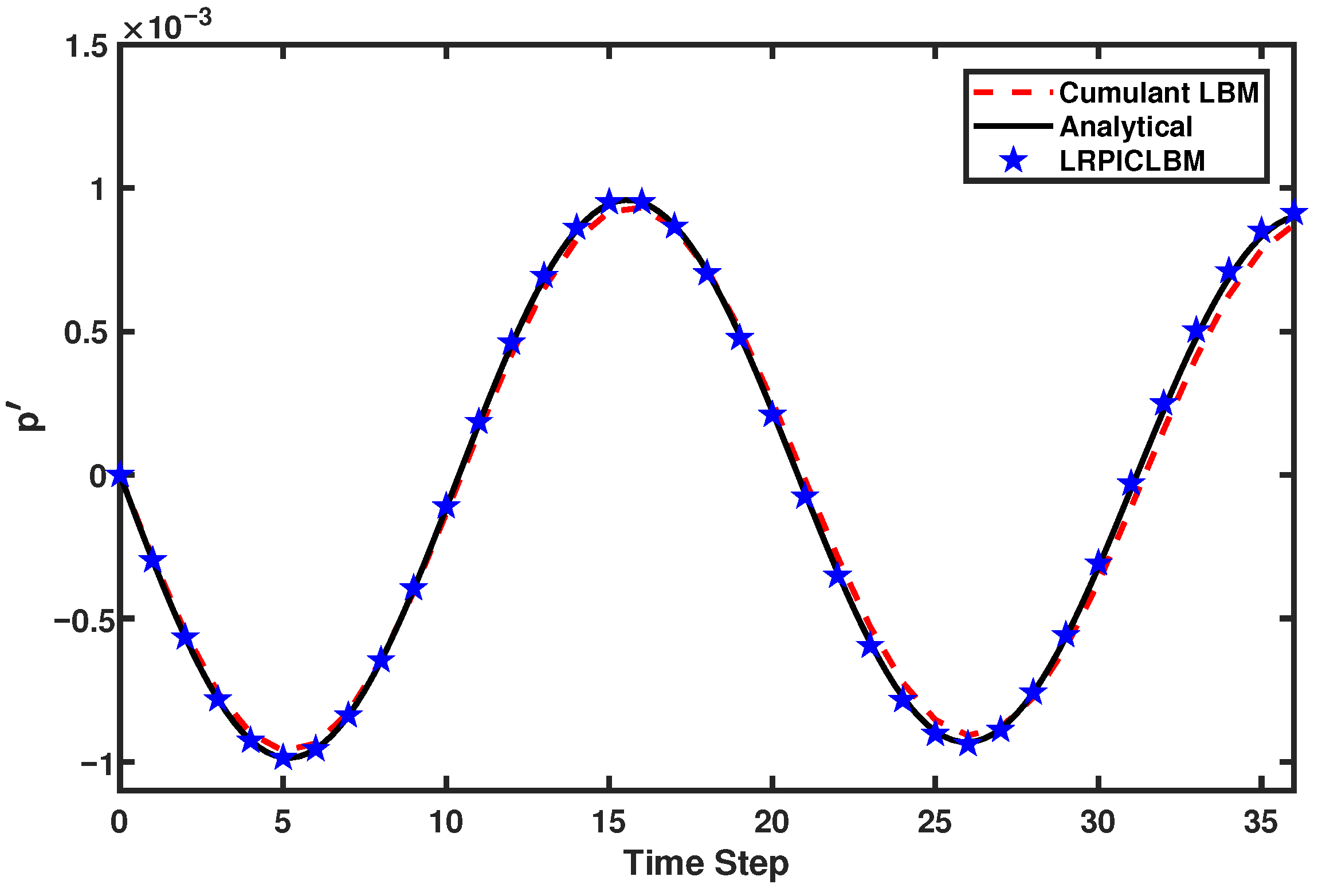
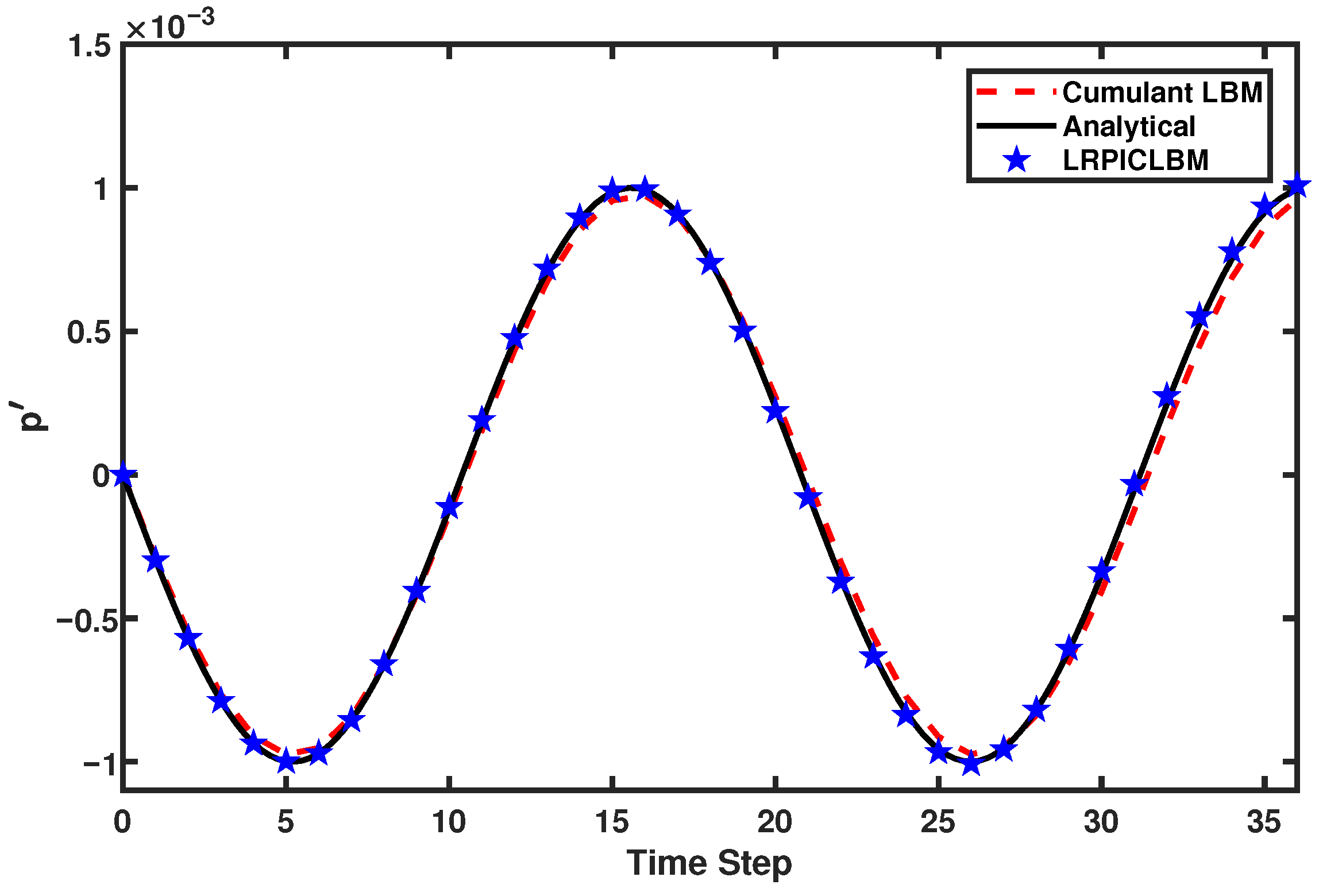
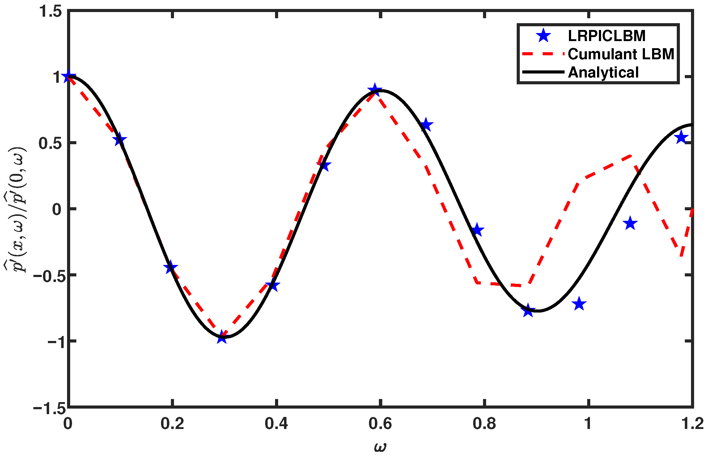
3.1. Planar Standing Wave

As an initial case study, we performed a temporal analysis on a standing plane acoustic wave in a periodic domain. The dissipation and dispersion relations based on the temporal analysis of Equation (26) are [25]
c T = c s 1 k ν c s 2
α T = k 2 ν
where k is the wave number. The assumptions for this set-up are presented in Table 1. They were chosen as in reference [26] for ease of comparison.
The acoustic pressure at time t is [26]
p ( x , y , t ) = A exp α T t sin k x c T t
It should be noted that the results of the temporal analysis can be considered as a function of the number of points per wavelength N p p w = λ / Δ x or the non-dimensional wave-number k Δ x = 2 π / N p p w .
In accordance with the concepts discussed in [26] to study the accuracy of the propagation of waves using the local radial point interpolation cumulant lattice Boltzmann method (LRPIC-LBM), various viscosities and different resolutions (i.e., the number of points per wavelength) were studied. Figure 2 shows the acoustic pressure time history for ν = 1.0 × 10 2 ( Δ x 2 Δ t ) with N p p w = 12 points per wavelength. The analytical result is represented by a solid black line, whereas the cumulant LBM and the LRPIC-LBM are shown with a red dashed line and a blue five-pointed star, respectively. The deviations of the numerical phase speed and the temporal dissipation rate from the theoretical values are less than one percent for the BGK LBM [25] and the cumulant LBM [26] for resolutions lower than 12 points per wavelength. However, the LRPIC-LBM exhibits even better behavior in predicting the acoustic pressure of the analytical values.
The acoustic pressure time history for ν = 1.0 × 10 4 ( Δ x 2 Δ t ) with N p p w = 12 points per wavelength is presented in Figure 3. It shows the comparison between the analytical solution, the cumulant LBM and the LRPIC-LBM numerical solution at low viscosities. One of the most problematic issues in the BGK LBM is the low viscosity limit, which makes the solution unstable. However, the cumulant LBM, with phase speed and temporal dissipation rate errors of less than 1 percent, as in reference [26], did not present difficulties at low viscosity. Although both approaches were successful, the new method exhibited better performance, closely following the theoretical result for the same viscosity value.
An important characteristic highlighted by some researchers [25,26] is that these numerical deviations are only a function of N p p w and are independent of other parameters such as frequency and viscosity. They found that the errors of the BGK [25] and the cumulant LBM [26] are about 7 percent for N p p w = 4 . However, the acoustic pressure time history for ν = 1.0 × 10 2 ( Δ x 2 Δ t ) with N p p w = 4 points per wavelength illustrated in Figure 4 for the analytical solution, the cumulant LBM and the LRPIC-LBM reveals that the deviation is less than 2 percent for the LRPIC-LBM, with Δ t = 0.25 . Thus, the LRPIC-LBM is much more successful in predicting theoretical results even with a low number of points per wavelength.
The choice of the time step size has an influence on the accuracy and stability of the solution. A smaller time step leads to more accurate results, especially in a hyperbolic partial differential Equation (PDE). To minimize the phase speed and dissipation rate errors, the time step was reduced. Figure 5 shows the acoustic pressure time history for ν = 1.0 × 10 2 ( Δ x 2 Δ t ) with N p p w = 4 points per wavelength and Δ t = 0.1 . The LRPI-CLBM replicates the analytical results with negligible errors. Therefore, this method makes it possible to predict wave motion more accurately with no dependency on the number of points per wavelength N p p w .
Although the results of the propagation of acoustic waves for regular nodal distributions were good, it is important to adequately estimate accuracy when considering irregular nodes (Figure 1b). The acoustic pressure time history for ν = 1.0 × 10 2 ( Δ x 2 Δ t ) with N p p w = 12 points per wavelength is presented in Figure 6. The results show that the local radial point interpolation cumulant lattice Boltzmann method (LRPIC-LBM) with irregular nodal distributions again very closely reproduced the analytical acoustic pressure.

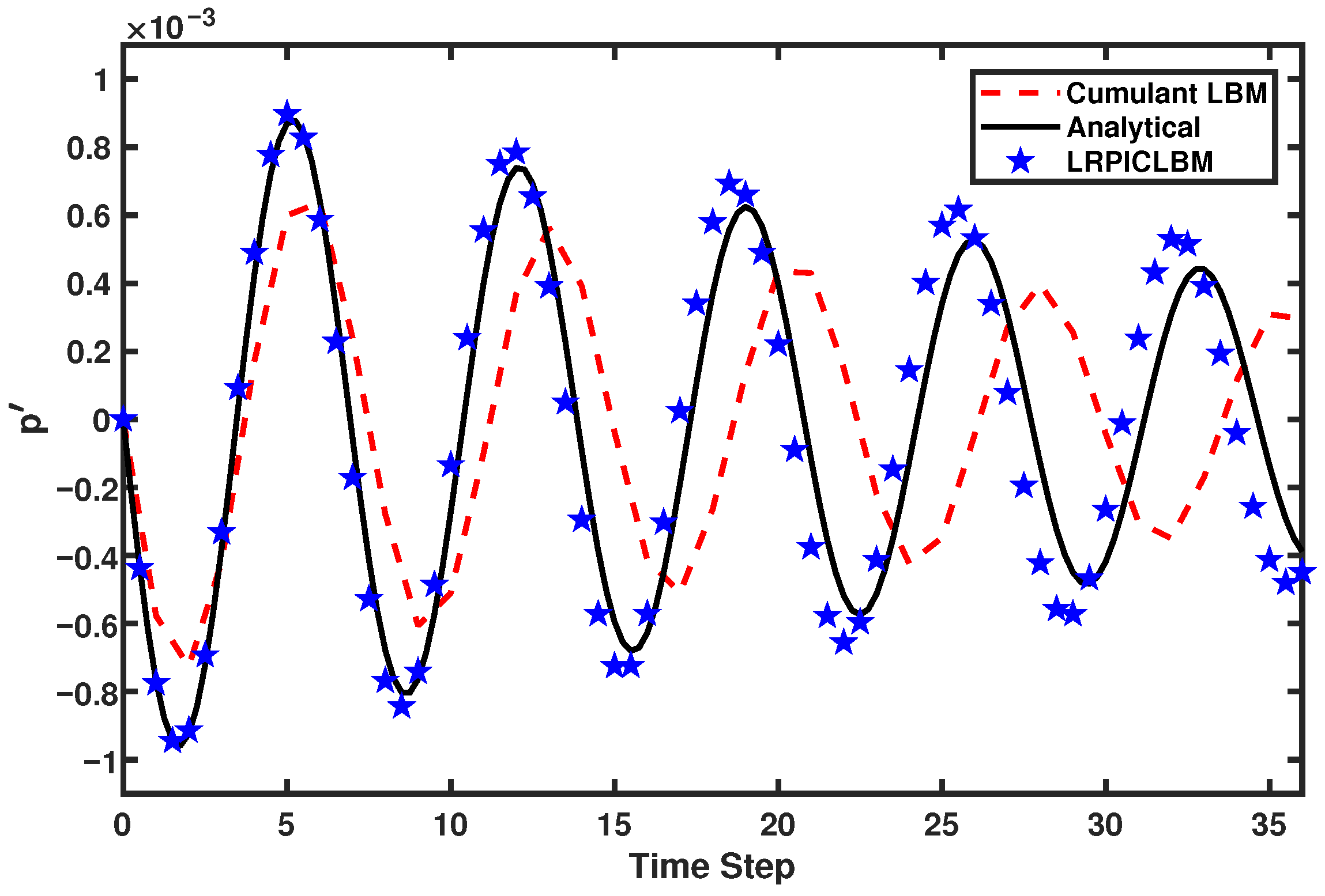
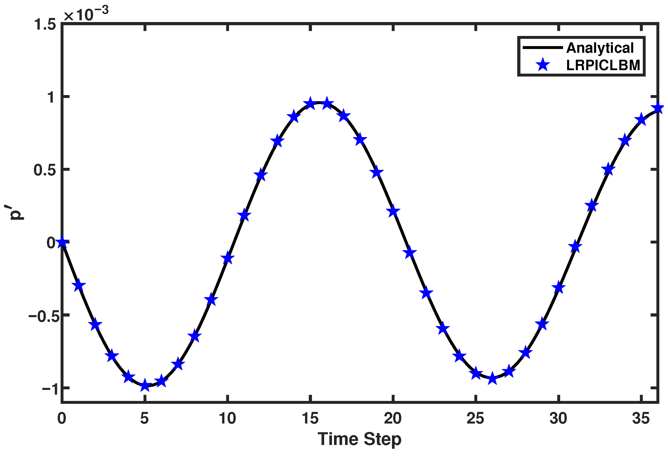
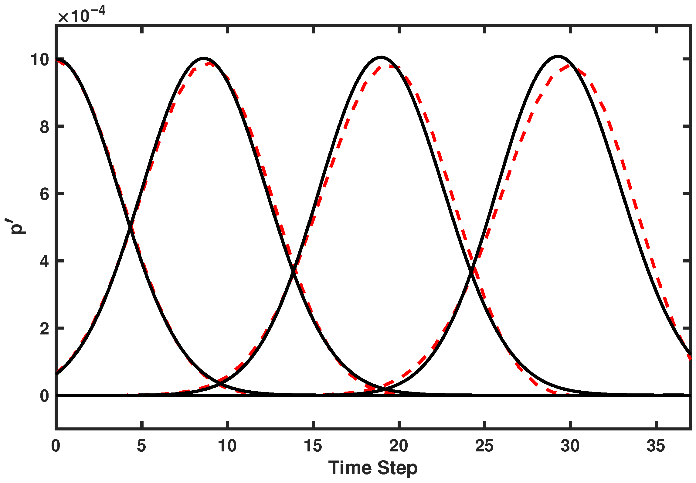
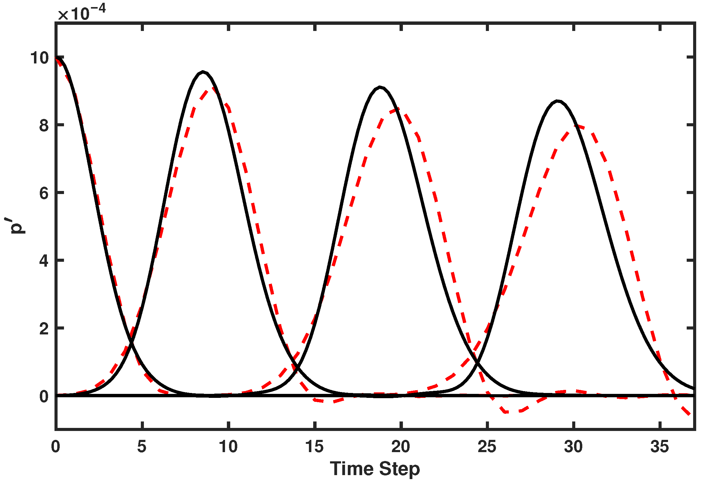
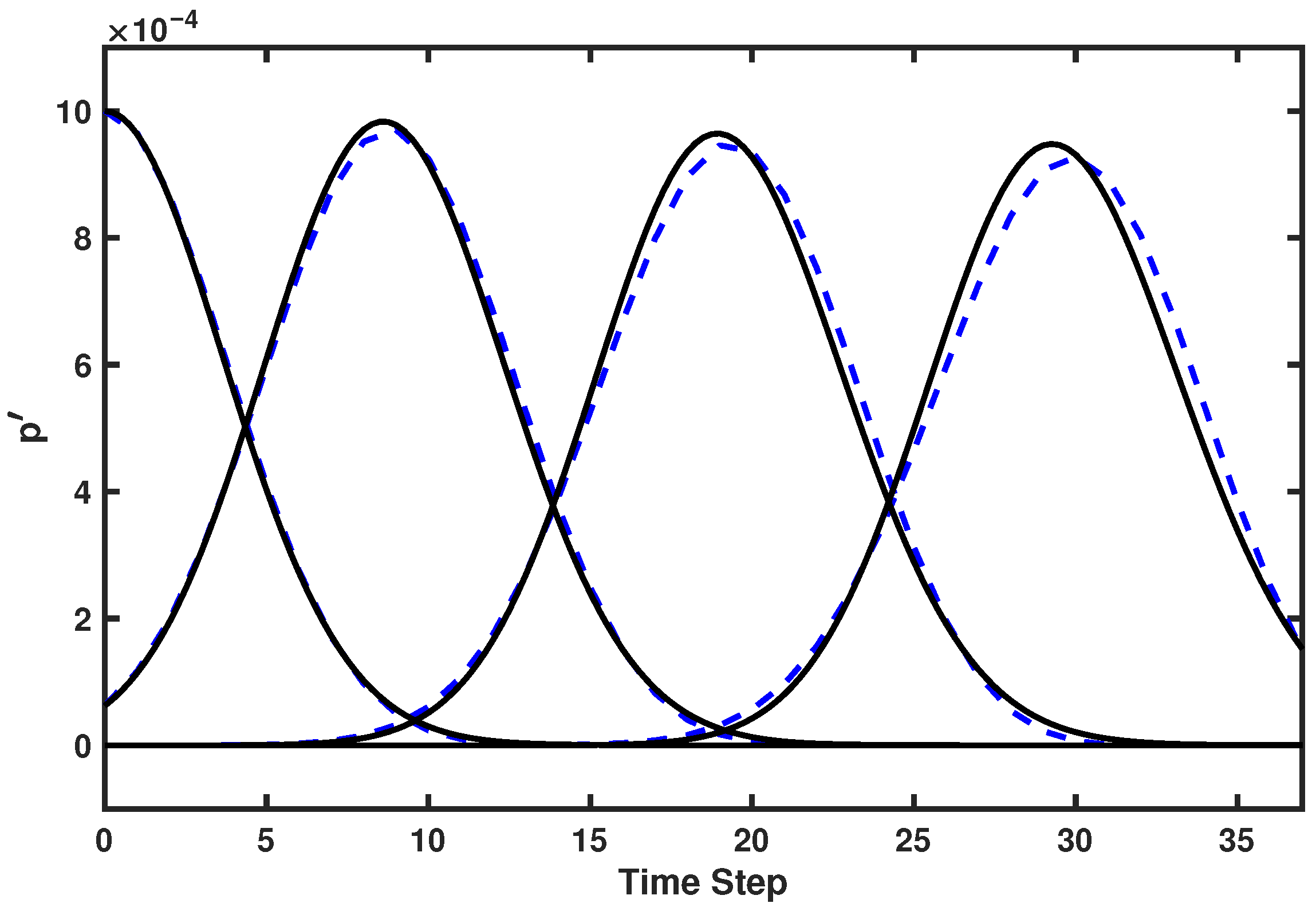
3.2. Planar Pulse Wave

Next, we studied a planar pulse wave by replacing the plane wave with a Gaussian shape planar pulse, initially located at the center of the domain. The dissipation and dispersion relationships derived from the spatial analysis of Equation (26) are [25]
c S = 2 c s 1 + ω τ s 2 1 + ω τ s 2 + 1
α S = ω 2 c s 1 + ω τ s 2 1 1 + ω τ s 2
The variables and parameters for this case are presented in Table 2. A planar pulse emits from the origin throughout the domain, where periodic boundary conditions are imposed.
To assess the accuracy of the LRPIC-LBM in simulating the pulse wave emission, we proceeded as in reference [26]. Different viscosities and resolutions (which are related to the choice of σ ) were studied. Figure 7 depicts the acoustic pressure time history for ν = 1.0 × 10 2 ( Δ x 2 Δ t ) with σ = 0.1 . The cumulant LBM results (dashed red line) are compared to the LRPIC-LBM (solid black line). As stated in [25,26] the intensity loss at any location is proportional to the distance of propagation, regardless of the precise location. Thus, the data were extracted from the center of the domain, and at 5, 11, and 17 nodes apart from the center. For resolutions up to σ = 0.1 , deviations between the cumulant LBM and the LRPIC-LBM results were less than 1 percent.
The acoustic pressure time history for ν = 1.0 × 10 4 ( Δ x 2 Δ t ) with σ = 0.1 is shown in Figure 8. It presents the comparison between the cumulant LBM and the LRPIC-LBM at low viscosity. While the standard BGK LBM creates instabilities and noisy results, less than 1 percent deviation was found between the cumulant LBM and this method, with stable behavior at low viscosities. In addition, as in the case of the temporal results shown in Figure 3, reducing the viscosity in the considered range did not substantially impact the results.
Like the parameter N p p w introduced in the temporal analysis of the first set up, σ is another effective parameter used in spatial analysis which affects the accuracy of the LBM results.The acoustic pressure time history is depicted in Figure 9 for ν = 1.0 × 10 2 ( Δ x 2 Δ t ), with σ = 0.06 . It shows that the deviations between the cumulant LBM and the LRPIC-LBM results increase after the reduction of σ . The wiggling observed in the results of the cumulant LBM is due to the reduction of the number of nodes inside the pulse, which brings the accuracy of the results into question. However, the LRPIC-LBM graphs are smooth and unaffected by the lesser number of nodes. To better assess the accuracy of the LRPIC-LBM compared to the cumulant LBM, the data shown in Figure 9 were compared with the analytical results. The Fourier transform of the pressure time history of the passing wave yields the Fourier coefficient of pressure p ^ x , ω = p ^ x , 0 exp α S x exp i ω x c S which is the solution to Equation (26) [25]. Figure 10 shows the ratio p ^ x , ω / p ^ x , 0 as a function of angular frequency for the analytical solution. This figure shows that the LRPIC-LBM is more successful than the cumulant LBM at predicting theoretical results with σ = 0.06 . Thus, this method can model wave propagation more accurately even at smaller resolutions.
Figure 11 illustrates the acoustic pressure time history for ν = 1.0 × 10 2 ( Δ x 2 Δ t ) with σ = 0.1 considering irregular nodes (Figure 1b). The cumulant LBM and the LRPIC-LBM results are represented by a dashed blue line and a solid black line, respectively. The data are extracted as in Figure 7. The results show that the LRPIC-LBM with irregular nodal distributions reproduced the behavior observed previously.

4. Conclusions

This paper presents a numerical study of the propagation of acoustic waves, one of the challenging issues occurring in wind turbine simulations, that includes the temporal decay of a standing plane wave and the spatial decay of a planar acoustic pulse, using the local radial point interpolation cumulant lattice Boltzmann method (LRPIC-LBM). The LB equation is divided into collision, modeled by the cumulant method, and streaming, discretized in time and space, using the Lax–Wendroff scheme and the local radial point interpolation method (RPIM). The LRPIC-LBM results were compared with the cumulant LBM and the analytical solutions. Both methods showed a similar acoustic pressure time history, and the deviations for the phase speed and the dissipation rate were minor for high number of points per wavelength N p p w and resolution σ . In addition, they showed that reduced viscosity does not affect the stability of either LB method due to the intrinsic characteristics of the cumulant method. Unlike LB methods such as the BGK LBM and the cumulant LBM, the time history for the acoustic pressure and the phase speed and dissipation rate predicted by LRPIC-LBM showed considerably smaller errors for low N p p w and σ due to the construction of the meshless method itself. Moreover, the LRPIC-LBM with irregular nodal distributions reproduces the same propagation of acoustic waves obtained with regular nodal distributions.
In summary, the freedom to scatter nodes based on problem conditions and the occurrence of sharp gradients plus the accuracy obtained from the RPIM along with the good stability and simplicity achieved by the cumulant LBM may provide an adequate platform with which to model wind turbine problems.

Author Contributions

Conceptualization: M.G., C.S., I.C. and E.K.F.; methodology, M.G., C.S., I.C. and E.K.F.; coding, M.G., C.S., I.C. and E.K.F.; validation, M.G., C.S., I.C. and E.K.F.; formal analysis, M.G., C.S., I.C. and E.K.F.; investigation, M.G., C.S., I.C. and E.K.F.; resources, M.G., C.S., I.C. and E.K.F.; data curation, M.G., C.S., I.C. and E.K.F.; writing—original draft preparation, M.G.; writing—review and editing, C.S., I.C. and E.K.F.; visualization, M.G., C.S., I.C. and E.K.F.; supervision, C.S. and I.C.; project administration, C.S. and I.C.; funding acquisition, C.S. and I.C. All authors contributed equally to this work. All authors have read and agreed to the published version of the manuscript.

Funding

This work has been funded by the Spanish Ministry of Economy, Industry and Competitiveness Research National Agency (under project DPI2016-75791-C2-1-P), by FEDER funds and by Generalitat de Catalunya - AGAUR (under project 2017 SGR 01234).

Institutional Review Board Statement

Not applicable.

Informed Consent Statement

Not applicable.

Data Availability Statement

Not applicable.

Conflicts of Interest

The authors declare no conflict of interest.

Abbreviations

The following abbreviations are used in this manuscript:
LRPIC-LBMLocal radial point interpolation cumulant lattice Boltzmann method
LBMLattice Boltzmann method
RPIMRadial point interpolation method
NRELNational Renewable Energy Laboratory
NWTCNational Wind Technology Center
CAAComputational aeroacoustic
DRPDispersion relation preserving scheme
GODRPGrid optimized dispersion relation preserving schemes
BGK-LBMBhatnagar Gross Krook lattice Boltzmann method
LBM-rrBGKLattice Boltzmann method recursive regularized Bhatnagar Gross Krook
IS-LBMInterpolation supplemented lattice Boltzmann method
FDLBEFinite difference lattice Boltzmann equation
FVLBEFinite volume lattice Boltzmann Equation
FELBEFinite element lattice Boltzmann equation
TLLBMTaylor-series expansion and least-squares-based lattice Boltzmann method
FSIFluid structure interaction
FDMFinite difference method
SPHSmoothed particle hydrodynamics
LPIMLocal point interpolation method
LRPIMLocal radial point interpolation method
MLPGMeshless local Petrov–Galerkin method
MRTMulti-relaxation times
PDFProbability density function
PIMPoint interpolation method
RBFRadial basis functions
MQMulti-quadrics
WRWeighted residuals
PDEPartial differential equation

References

  1. Burton-Jones, A. Knowledge Capitalism: Business, Work, and Learning in the New Economy; Oxford University Press: Oxford, UK, 2001. [Google Scholar]
  2. Letcher, T.M. Wind Energy Engineering: A Handbook for Onshore and Offshore Wind Turbines; Academic Press: Cambridge, MA, USA, 2017. [Google Scholar]
  3. Bowdler, D.; Leventhall, H. Wind Turbine Noise; Multi-Science Pub.: Brentwood, CA, USA, 2011. [Google Scholar]
  4. Wagner, S.; Bareiss, R.; Guidati, G. Wind Turbine Noise; Springer Science & Business Media: Berli/Heidelberg, Germany, 2012. [Google Scholar]
  5. Singer, B.A.; Lockard, D.P.; Brentner, K.S. Computational aeroacoustic analysis of slat trailing-edge flow. AIAA J. 2000, 38, 1558–1564. [Google Scholar] [CrossRef]
  6. Manwell, J.F.; McGowan, J.G.; Rogers, A.L. Wind Energy Explained: Theory, Design and Application; John Wiley & Sons: Hoboken, NJ, USA, 2010. [Google Scholar]
  7. Geier, M.; Kian Far, E. A Sliding Grid Method For The Lattice Boltzmann Method Using Compact Interpolation. In Proceedings of the The First International Workshop on Lattice Boltzmann for Wind Energy, Online Conference, 25–26 February 2021. [Google Scholar]
  8. Morris, P.; Long, L.; Brentner, K. An aeroacoustic analysis of wind turbines. In Proceedings of the 42nd AIAA Aerospace Sciences Meeting and Exhibit, Reno, NV, USA, 5–8 January 2004; p. 1184. [Google Scholar]
  9. Robinson, M.C.; Hand, M.; Simms, D.; Schreck, S. Horizontal Axis Wind Turbine Aerodynamics: Three-Dimensional, Unsteady, and Separated Flow Influences; Technical Report; National Renewable Energy Lab.: Golden, CO, USA, 1999.
  10. Tummala, A.; Velamati, R.K.; Sinha, D.K.; Indraja, V.; Krishna, V.H. A review on small scale wind turbines. Renew. Sustain. Energy Rev. 2016, 56, 1351–1371. [Google Scholar] [CrossRef]
  11. Spera, D.A. Wind Turbine Technology; Wind Energy Technologies Office: Washington, DC, USA, 1994.
  12. Tam, C.K. Computational aeroacoustics-Issues and methods. AIAA J. 1995, 33, 1788–1796. [Google Scholar] [CrossRef]
  13. Wells, V.L.; Renaut, R.A. Computing aerodynamically generated noise. Annu. Rev. Fluid Mech. 1997, 29, 161–199. [Google Scholar] [CrossRef] [Green Version]
  14. Kim, J.W.; Lee, D.J. Optimized compact finite difference schemes with maximum resolution. AIAA J. 1996, 34, 887–893. [Google Scholar] [CrossRef] [Green Version]
  15. Tam, C.K.; Webb, J.C. Dispersion-Relation-Preserving Schemes for Computational Aeroacoustics; NASA: Washington, DC, USA, 1992.
  16. Cheong, C.; Lee, S. Grid-optimized dispersion-relation-preserving schemes on general geometries for computational aeroacoustics. J. Comput. Phys. 2001, 174, 248–276. [Google Scholar] [CrossRef]
  17. Gröschel, E.; Schröder, W.; Renze, P.; Meinke, M.; Comte, P. Noise prediction for a turbulent jet using different hybrid methods. Comput. Fluids 2008, 37, 414–426. [Google Scholar] [CrossRef]
  18. Delfs, J.; Bertsch, L.; Zellmann, C.; Rossian, L.; Kian Far, E.; Ring, T.; Langer, S.C. Aircraft Noise Assessment—From Single Components to Large Scenarios. Energies 2018, 11, 429. [Google Scholar] [CrossRef] [Green Version]
  19. Colonius, T.; Lele, S.K.; Moin, P. The scattering of sound waves by a vortex: Numerical simulations and analytical solutions. J. Fluid Mech. 1994, 260, 271–298. [Google Scholar] [CrossRef] [Green Version]
  20. Mitchell, B.; Lele, S.; Moin, P. Direct computation of the sound from a compressible co-rotating vortex pair. In Proceedings of the 30th Aerospace Sciences Meeting and Exhibit, Reno, NV, USA, 6–9 January 1992; p. 374. [Google Scholar]
  21. Kian Far, E.; Geier, M.; Kutscher, K.; Krafczyk, M. Implicit Large Eddy Simulation of Flow in a Micro-Orifice with the Cumulant Lattice Boltzmann Method. Computation 2017, 5, 23. [Google Scholar] [CrossRef] [Green Version]
  22. Kian Far, E. A Cumulant LBM approach for Large Eddy Simulation of Dispersion Microsystems. Ph.D. Thesis, Universität Braunschweig, Braunschweig, Germany, 2015. [Google Scholar]
  23. Buick, J.; Greated, C.; Campbell, D. Lattice BGK simulation of sound waves. EPL (Europhysics Lett.) 1998, 43, 235. [Google Scholar] [CrossRef]
  24. Dellar, P.J. Bulk and shear viscosities in lattice Boltzmann equations. Phys. Rev. E 2001, 64, 031203. [Google Scholar] [CrossRef] [Green Version]
  25. Bres, G.; Pérot, F.; Freed, D. Properties of the lattice Boltzmann method for acoustics. In Proceedings of the 15th AIAA/CEAS Aeroacoustics Conference (30th AIAA Aeroacoustics Conference), Miami, FL, USA, 11–13 May 2009; p. 3395. [Google Scholar]
  26. Gorakifard, M.; Cuesta, I.; Salueña, C.; Kian Far, E. Acoustic Wave Propagation and its Application to Fluid Structure Interaction using the Cumulant Lattice Boltzmann Method. Comput. Math. Appl. 2021, 87, 91–106. [Google Scholar] [CrossRef]
  27. Latt, J.; Chopard, B. Lattice Boltzmann method with regularized pre-collision distribution functions. Math. Comput. Simul. 2006, 72, 165–168. [Google Scholar] [CrossRef]
  28. Malaspinas, O. Increasing stability and accuracy of the lattice Boltzmann scheme: Recursivity and regularization. arXiv 2015, arXiv:1505.06900. [Google Scholar]
  29. Brogi, F.; Malaspinas, O.; Chopard, B.; Bonadonna, C. Hermite regularization of the lattice Boltzmann method for open source computational aeroacoustics. J. Acoust. Soc. Am. 2017, 142, 2332–2345. [Google Scholar] [CrossRef]
  30. Chávez-Modena, M.; Martínez, J.; Cabello, J.; Ferrer, E. Simulations of aerodynamic separated flows using the lattice Boltzmann solver XFlow. Energies 2020, 13, 5146. [Google Scholar] [CrossRef]
  31. Filippova, O.; Hänel, D. Grid Refinement for Lattice-BGK Models. J. Comput. Phys. 1998, 147, 219–228. [Google Scholar] [CrossRef]
  32. Wood, S.L. Lattice Boltzmann Methods for Wind Energy Analysis. Ph.D. Thesis, University of Tennessee, Knoxville, TN, USA, 2016. [Google Scholar]
  33. Deiterding, R.; Wood, S.L. Predictive Wind Turbine Simulation with an Adaptive Lattice Boltzmann Method for Moving Boundaries; Journal of Physics: Conference Series; IOP Publishing: Bristol, UK, 2016; Volume 753, p. 082005. [Google Scholar]
  34. Gorakifard, M.; Salueña, C.; Cuesta, I.; Kian Far, E. Acoustical analysis of fluid structure interaction using the Cumulant lattice Boltzmann method. In Proceedings of the 16th International Conference for Mesoscopic Methods in Engineering and Science, Heriot-Watt University, Edinburgh, UK, 22–26 July 2019. [Google Scholar]
  35. Chen, Z.; Shu, C.; Tan, D.S. The simplified lattice Boltzmann method on non-uniform meshes. Commun. Comput. Phys 2018, 23, 1131. [Google Scholar] [CrossRef]
  36. He, X.; Luo, L.S.; Dembo, M. Some Progress in Lattice Boltzmann Method. Part I. Nonuniform Mesh Grids. J. Comput. Phys. 1996, 129, 357–363. [Google Scholar] [CrossRef] [Green Version]
  37. He, X.; Doolen, G. Lattice Boltzmann Method on Curvilinear Coordinates System: Flow around a Circular Cylinder. J. Comput. Phys. 1997, 134, 306–315. [Google Scholar] [CrossRef]
  38. Chen, H. Volumetric formulation of the lattice Boltzmann method for fluid dynamics: Basic concept. Phys. Rev. E 1998, 58, 3955–3963. [Google Scholar] [CrossRef]
  39. Mei, R.; Shyy, W. On the finite difference-based lattice Boltzmann method in curvilinear coordinates. J. Comput. Phys. 1998, 143, 426–448. [Google Scholar] [CrossRef]
  40. Xi, H.; Peng, G.; Chou, S.H. Finite-volume lattice Boltzmann method. Phys. Rev. E 1999, 59, 6202. [Google Scholar] [CrossRef] [PubMed] [Green Version]
  41. Nannelli, F.; Succi, S. The lattice Boltzmann equation on irregular lattices. J. Stat. Phys. 1992, 68, 401–407. [Google Scholar] [CrossRef]
  42. Peng, G.; Xi, H.; Duncan, C.; Chou, S.H. Finite volume scheme for the lattice Boltzmann method on unstructured meshes. Phys. Rev. E 1999, 59, 4675. [Google Scholar] [CrossRef]
  43. Lee, T.; Lin, C.L. A Characteristic Galerkin Method for Discrete Boltzmann Equation. J. Comput. Phys. 2001, 171, 336–356. [Google Scholar] [CrossRef]
  44. Li, Y.; LeBoeuf, E.J.; Basu, P.K. Least-squares finite-element scheme for the lattice Boltzmann method on an unstructured mesh. Phys. Rev. E 2005, 72, 046711. [Google Scholar] [CrossRef] [PubMed] [Green Version]
  45. Min, M.; Lee, T. A spectral-element discontinuous Galerkin lattice Boltzmann method for nearly incompressible flows. J. Comput. Phys. 2011, 230, 245–259. [Google Scholar] [CrossRef]
  46. Shu, C.; Niu, X.; Chew, Y. Taylor-series expansion and least-squares-based lattice Boltzmann method: Two-dimensional formulation and its applications. Phys. Rev. E 2002, 65, 036708. [Google Scholar] [CrossRef] [PubMed] [Green Version]
  47. Shu, C.; Chew, Y.; Niu, X. Least-squares-based lattice Boltzmann method: A meshless approach for simulation of flows with complex geometry. Phys. Rev. E 2001, 64, 045701. [Google Scholar] [CrossRef]
  48. Fard, E.G.; Shirani, E.; Geller, S. The Fluid Structure Interaction Using the Lattice Boltzmann Method. In Proceedings of the 13th Annual International Conference fluid dynamic conference, Shiraz, Iran, 26–28 October 2010. [Google Scholar]
  49. Liu, G.R.; Gu, Y.T. An Introduction to Meshfree Methods and Their Programming; Springer Science & Business Media: Berlin/Heidelberg, Germany, 2005. [Google Scholar]
  50. Liu, G. Meshfree Methods: Moving Beyond the Finite Element Method, Second Edition, 2nd ed.; CRC Press: Boca Raton, FL, USA, 2009; pp. 1–692. [Google Scholar]
  51. Liu, G.; Gu, Y. A local point interpolation method for stress analysis of two-dimensional solids. Struct. Eng. Mech. 2001, 11, 221–236. [Google Scholar] [CrossRef]
  52. Liu, G.; Gu, Y. A local radial point interpolation method (LRPIM) for free vibration analyses of 2-D solids. J. Sound Vib. 2001, 246, 29–46. [Google Scholar] [CrossRef] [Green Version]
  53. Atluri, S.N.; Zhu, T. A new meshless local Petrov-Galerkin (MLPG) approach in computational mechanics. Comput. Mech. 1998, 22, 117–127. [Google Scholar] [CrossRef]
  54. Li, Q.; Yang, H.; Yang, F.; Yao, D.; Zhang, G.; Ran, J.; Gao, B. Calculation of Hybrid Ionized Field of AC/DC Transmission Lines by the Meshless Local Petorv–Galerkin Method. Energies 2018, 11, 1521. [Google Scholar] [CrossRef] [Green Version]
  55. Musavi, S.H.; Ashrafizaadeh, M. Meshless lattice Boltzmann method for the simulation of fluid flows. Phys. Rev. E 2015, 91, 023310. [Google Scholar] [CrossRef] [PubMed]
  56. Musavi, S.H.; Ashrafizaadeh, M. Development of a three dimensional meshless numerical method for the solution of the Boltzmann equation on complex geometries. Comput. Fluids 2019, 181, 236–247. [Google Scholar] [CrossRef]
  57. Bawazeer, S. Lattice Boltzmann Method with Improved Radial Basis Function Method. Ph.D. Thesis, University of Calgary, Calgary, AB, Canada, 2019. [Google Scholar]
  58. Tanwar, S. A meshfree-based lattice Boltzmann approach for simulation of fluid flows within complex geometries: Application of meshfree methods for LBM simulations. In Analysis and Applications of Lattice Boltzmann Simulations; IGI Global: Hershey, PA, USA, 2018; pp. 188–222. [Google Scholar]
  59. Kian Far, E.; Geier, M.; Krafczyk, M. Simulation of rotating objects in fluids with the cumulant lattice Boltzmann model on sliding meshes. Comput. Math. Appl. 2018. [Google Scholar] [CrossRef]
  60. Kian Far, E.; Geier, M.; Kutscher, K.; Konstantin, M. Simulation of micro aggregate breakage in turbulent flows by the cumulant lattice Boltzmann method. Comput. Fluids 2016, 140, 222–231. [Google Scholar] [CrossRef]
  61. Kian Far, E.; Langer, S. Analysis of the cumulant lattice Boltzmann method for acoustics problems. In Proceedings of the 13th International Conference on Theoretical and Computational Acoustics, Vienna, Austria, 31 July–3 August 2017. [Google Scholar]
  62. Geier, M. Ab Initio Derivation of the Cascaded Lattice Boltzmann Automaton. Ph.D. Thesis, University of Freiburg–IMTEK, Freiburg, Germany, 2006. [Google Scholar]
  63. Geier, M.; Greiner, A.; Korvink, J.G. Reference Frame Independent Partitioning of the Momentum Distribution Function in Lattice Boltzmann Methods with Multiple Relaxation Rates; University of Freiburg: Freiburg, Germany, 2008. [Google Scholar]
  64. Seeger, S.; Hoffmann, H. The cumulant method for computational kinetic theory. Contin. Mech. Thermodyn. 2000, 12, 403–421. [Google Scholar] [CrossRef]
  65. Seeger, S.; Hoffmann, K. The cumulant method for the space-homogeneous Boltzmann equation. Contin. Mech. Thermodyn. 2005, 17, 51–60. [Google Scholar] [CrossRef]
  66. Kian Far, E.; Geier, M.; Kutscher, K.; Krafczyk, M. Distributed cumulant lattice Boltzmann simulation of the dispersion process of ceramic agglomerates. J. Comput. Methods Sci. Eng. 2016, 16, 231–252. [Google Scholar] [CrossRef]
  67. Kian Far, E. A sliding mesh LBM approach for the simulation of the rotating objects. In Proceedings of the 13th International Conference for Mesoscopic Methods in Engineering and Science, Hamburg, Germany, 18–22 July 2016. [Google Scholar]
  68. Geier, M.; Schönherr, M.; Pasquali, A.; Krafczyk, M. The cumulant lattice Boltzmann equation in three dimensions: Theory and validation. Comput. Math. Appl. 2015, 70, 507–547. [Google Scholar] [CrossRef] [Green Version]
  69. Kian Far, E. Turbulent Flow Simulation of Dispersion Microsystem with Cumulant Lattice Boltzmann Method, FORMULA X. 24 June 2019. Available online: https://www.formulation.org.uk/images/stories/FormulaX/Posters/P-27.pdf (accessed on 2 March 2021).
  70. Schäfer, R.; Böhle, M. Validation of the Lattice Boltzmann Method for Simulation of Aerodynamics and Aeroacoustics in a Centrifugal Fan. In Acoustics; Multidisciplinary Digital Publishing Institute: Basel, Switzerland, 2020; Volume 2, pp. 735–752. [Google Scholar]
  71. Ye, Q.; Avallone, F.; Van Der Velden, W.; Casalino, D. Effect of Vortex Generators on NREL Wind Turbine: Aerodynamic Performance and Far-Field Noise; Journal of Physics: Conference Series; IOP Publishing: Bristol, UK, 2020; Volume 1618, p. 052077. [Google Scholar]
  72. Kinsler, L.E.; Frey, A.R.; Coppens, A.B.; Sanders, J.V. Fundamentals of Acoustics; John Wiley & Sons: Hoboken, NJ, USA, 1999. [Google Scholar]
Figure 1. Nodal arrangement for the propagation of planar acoustic waves in LRPIC-LBM simulations: (a) Regular nodes. (b) Irregular nodes.
Energies 14 01443 g001
Figure 2. Acoustic pressure ( k g Δ x Δ t 2 ) versus time step ( Δ t ) for ν = 1.0 × 10 2 ( Δ x 2 Δ t ) with N p p w = 12 points per wavelength.
Energies 14 01443 g002
Figure 3. Acoustic pressure ( k g Δ x Δ t 2 ) versus time step ( Δ t ) for ν = 1.0 × 10 4 ( Δ x 2 Δ t ) with N p p w = 12 points per wavelength.
Energies 14 01443 g003
Figure 4. Acoustic pressure ( k g Δ x Δ t 2 ) versus time step ( Δ t ) for ν = 1.0 × 10 2 ( Δ x 2 Δ t ) with N p p w = 4 points per wavelength with Δ t = 0.25 .
Energies 14 01443 g004
Figure 5. Acoustic pressure ( k g Δ x Δ t 2 ) versus time step ( Δ t ) for ν = 1.0 × 10 2 ( Δ x 2 Δ t ) with N p p w = 4 points per wavelength with Δ t = 0.1 .
Energies 14 01443 g005
Figure 6. Acoustic pressure ( k g Δ x Δ t 2 ) versus time step ( Δ t ) for ν = 1.0 × 10 2 ( Δ x 2 Δ t ) with N p p w = 12 points per wavelength with irregular nodal distributions.
Energies 14 01443 g006
Figure 7. Acoustic pressure ( k g Δ x Δ t 2 ) versus time step ( Δ t ) for ν = 1.0 × 10 2 ( Δ x 2 Δ t ) with σ = 0.1 : the cumulant LBM (dashed red line), LRPIC-LBM (solid black line).
Energies 14 01443 g007
Figure 8. Acoustic pressure ( k g Δ x Δ t 2 ) versus time step ( Δ t ) for ν = 1.0 × 10 4 ( Δ x 2 Δ t ) with σ = 0.1 : the cumulant LBM (dashed red line), LRPIC-LBM (solid black line).
Energies 14 01443 g008
Figure 9. Acoustic pressure( k g Δ x Δ t 2 ) versus time step ( Δ t ) for ν = 1.0 × 10 2 ( Δ x 2 Δ t ) with σ = 0.06 : the cumulant LBM (dashed red line), LRPIC-LBM (solid black line).
Energies 14 01443 g009
Figure 10. The ratio p ^ x , ω / p ^ x , 0 as a function of angular frequency ( 1 Δ t ) for the analytical solution, the cumulant LB and the LRPIC-LB methods.
Energies 14 01443 g010
Figure 11. Acoustic pressure ( k g Δ x Δ t 2 ) versus time step ( Δ t ) for ν = 1.0 × 10 2 ( Δ x 2 Δ t ) with σ = 0.1 considering irregular nodal distributions: the cumulant LBM (dashed blue line), LRPIC-LBM (solid black line).
Energies 14 01443 g011
Table 1. Parameters for the planar standing wave.
Variables p ( x , y , 0 ) ρ u v A
Description A sin 2 π x λ p ç s 2 p ρ 0 ç s 0 10 3 p 0
Table 2. Parameters for the planar pulse wave.
Variables p ( x , y , 0 ) ρ u v A σ
Description A exp ln 2 x 2 σ 2 p ç s 2 p ρ 0 ç s 0 10 3 p 0 0.06 0.1
Publisher’s Note: MDPI stays neutral with regard to jurisdictional claims in published maps and institutional affiliations.

