Snow-Induced PV Loss Modeling Using Production-Data Inferred PV System Models

Abstract

Snow-induced photovoltaic (PV)-energy losses (snow losses) in snowy and cold locations vary up to 100% monthly and 34% annually, according to literature. Levels that illustrate the need for snow loss estimation using validated models. However, to our knowledge, all these models build on limited numbers of sites and winter seasons, and with limited climate diversity. To overcome this limitation in underlying statistics, we investigate the estimation of snow losses using a PV system’s yield data together with freely available gridded weather datasets. To develop and illustrate this approach, 263 sites in northern Sweden are studied over multiple winters. Firstly, snow-free production is approximated by identifying snow-free days and using corresponding data to infer tilt and azimuth angles and a snow-free performance model incorporating shading effects, etc. This performance model approximates snow-free monthly yields with an average hourly standard deviation of 6.9%, indicating decent agreement. Secondly, snow losses are calculated as the difference between measured and modeled yield, showing annual snow losses up to 20% and means of 1.5–6.2% for winters with data for at least 89 sites. Thirdly, two existing snow loss estimation models are compared to our calculated snow losses, with the best match showing a correlation of 0.73 and less than 1% bias for annual snow losses. Based on these results, we argue that our approach enables studying snow losses for high numbers of PV systems and winter seasons using existing datasets.

1. Introduction

As costs for photovoltaic (PV) modules and systems continuously drop, PV is becoming increasingly mainstream and widespread. The technology expands ever more in geographical regions and climates with lower annual irradiations and with significant snowfall, such as Scandinavia and Canada [1,2].

With the expansion of new PV markets, the interest in climate-specific impacts also seems to increase, including impacts from snowfall on PV production. In a number of studies from snow-rich locations with cold winters, PV systems are found to suffer annual energy output losses up to 34% for certain years and systems, with monthly losses up to 100% [3,4,5,6,7]. Moreover, in moderate climates, significant loss levels around 5–6% typically, and up to 9.3%, have been reported, whereas plants in mild climates show typical annual losses below 2–3% [3,8,9,10]. These studies and their reported levels indicate that snow losses can have a substantial impact on the energy yield, in addition to impacting the financial conditions for the site investor and owner. Therefore, snow impacts should reasonably be taken into account during the planning of PV sites and be included in quotations and financial return on investment (ROI) or lifecycle cost of energy (LCoE) calculations.

The extent to which a PV array is covered with snow during winter is clearly depending on climate and—at a more detailed level—on weather conditions present before, during, and after snowfall. The surface temperature of the modules, whether the module surface is wet or dry, and the type of snow (wet or dry) impact the extent of accumulation of falling snow on the modules [11,12]. Once a module array is covered by snow, air temperature and irradiation levels and snow type play a crucial role in the speed of natural clearing of the modules by sliding or melting [9,11]. Furthermore, design parameters and technical specifics of the plant impact the speed of snow clearance. In general, higher tilt angles lead to shorter periods of snow coverage, but not in a linear relation. Townsend and Powers [6] suggested a linear relationship with the squared cosine of the tilt angle for annual losses, while Marion et al. [10] proposed a linear relationship to the sine of the tilt angle for the speed of snow sliding. Moreover, the smoothness of the array surface affected by module framing or mounting system parts [3,11] and interference with ground or roof constructions below the array [3,5,6,10] were reported to have a significant impact on snow clearance rates. Townsend and Powers [6] defined a basic approach to model ground interference, but for rooftop systems, many more parameters are likely to impact the interference, such as roof tilt angle, the possible presence of snow racks, module mounting height, type of roof cladding, and distance between the bottom of the array and the roof eaves.

In addition to the fraction of a PV module or array that is covered by snow, the spatial distribution in relation to string and module substring configurations also defines the resulting electrical power loss. The impact of snow coverage is similar to the impact of shading, or soiling in general, and includes the thickness and light transmittance of the snow cover [3,12]. Because snow is cleared by a combination of melting and sliding, it tends to cover only a part of the module and array, mostly reported to be the bottom of modules [9,12], but not limited to this area. In the latter case, snow from the bottom part of one module row is observed to slide downwards onto the top part of the underlying module row in the same array [13]. Based on these observations, the use of landscape orientation of modules seems to be beneficial because module bypass diodes typically divide modules into substrings in parallel to their long edge. However, early observations in an ongoing study indicate that snow sliding might be affected negatively due to module frames and inter-module gaps occurring at smaller intervals [14]. No conclusions on the final, combined effect of the two factors—bypass diodes and clearance speeds—can be drawn from current literature.

Several approaches to model snow coverage and/or snow losses have been developed, most of them being empirical and a few based on modeling physical principles [3]. Pawluk [3] presented an overview of models that are included in

Table 1. Overview of models for long-term prediction of snow losses, either directly (designated “Power” under Model Type) or through snow cover predictions (denoted as “Cover”).

Author (s)	Model Type	Number of PV Systems 1	Number of Winters
Powers et al. [4]	Power; Empirical	3; 1 location	1
Townsend and Powers [6]	Power; Empirical	4; 2 locations	2
Andrews et al. [9]	Power; Empirical	1	2
Hong et al. [15]	Power; Empirical	70	Up to 4
Zamo et al. [17]	Power; Empirical	28	2
Shishavan et al. [18]	Power; Empirical	2	3
Van Noord et al. [7]	Power; Empirical	6; 3 locations	2
Ross [11]	Cover; Principal	n/a	n/a
Lorenz et al. [19]	Cover; Empirical	14 (77)	1
Marion et al.; Ryberg and Freeman [10,16]	Cover; Empirical	6 (3); 2 locations	2 (1)
Bosman and Darling [20]	Cover; Empirical	(1)	2
Rahmatmand [21]	Cover; Principal	n/a	n/a

¹ The number used in empirical model development. Where applicable, the number of systems used in model validation is listed in parenthesis.

—with a single addition—to summarize the extent of the underlying data. Most approaches directly focus on predicting the impacts on PV energy generation, while other models predict snow coverage and from there estimate the expected energy yield. All listed empirical models show improvements in prediction accuracy, compared to prediction methods not considering snow losses at all, for the sites studied or used in validation. Prediction improvements are, however, not always consistent for all time resolutions, showing decent correspondence for annual estimates and large errors for monthly estimates or higher resolution estimates [6,10,15]. For example [15,16] presented annual absolute errors within 2% and 4% (of annual energy yield), respectively, and monthly absolute errors within 85% and 34% (of monthly observed energy yield), respectively.

Table 1 shows that most studies have a clearly limited statistical base, with limitations in one or more of the following three parameters: number of PV plants, geographical distribution, i.e., (micro-)climates, and number of winter seasons. This statistical limitation creates uncertainty regarding the general applicability and a need for broad validation efforts, extending all of the three mentioned parameters. Three studies include larger amounts of PV plants [15,17,19]. The study by Hong et al. [15] also had a relatively high number of winter seasons but was geographically limited to one city area (Seoul, Korea). Zamo et al. [17] geographically covered two counties in France—one a hilly region near a mountainous area and the other flatlands near the sea. The models tested in [17] were ignorant of any PV systems’ specifics and were all regressive, focusing mostly on advanced regression methods. The best model in general showed root-mean-square errors (RMSE) of 9–12% for hourly values three days ahead, but no specific results for the snowy seasons were presented. Lorenz et al. [19] covered northeast Germany (basically, the area of former East Germany) and showed a decrease of RMSE from 11% of installed power to around 7.5% for intra-day hourly prediction values at a single site level when implementing an assumed 100% snow cover for hours with air temperature below zero (0 °C).

The usefulness of a temperature threshold of 0 °C for snow coverage was confirmed by [3,10,16], though [3] noted that such a threshold should be combined with the use of snow cover conditions in order to prevent underestimation of snow losses during cold periods.

Out of all discussed prediction models, only the model by Marion et al. [10], with some minor adjustments [16], has been implemented in a publicly available PV simulation tool, namely in the National Renewable Energy Laboratory (NREL) System Advisor Model (SAM) [22].

The work presented in this article is aimed to extend data collection size (number of sites, number of years) by using generally available data to arrive at snow loss estimates that can be used to verify existing snow loss models and investigate new or improved modeling approaches. To succeed with this aim, it is critical to find reliable methods to infer snow-free performance, and it is preferable to identify inference methods for many of the main site-specific parameters.

We have found that satisfying snow-free models can be inferred for most PV systems. Inference of tilt and azimuth angles is possible with room for improvement. We can also show that estimated annual snow loss levels are in line with earlier publications and showing correlation with the model by Marion et al. with adjustments by Ryberg and Freeman [10,16].

2. Materials and Methods

2.1. Data Sources and Acquisition

This study uses data of PV sites with three different levels of available meta-data, which are referred to as reference sites, survey sites, and basic sites.

Table 2. Overview of sites included in the study and the data collected or available.

	Reference Sites	Survey Sites 1	Basic Sites
Number of sites	5	102	296
Meta-data
Peak power	X	X	X
Location (lat, lon)	X	X	X
Array tilt	X	X
Array azimuth	X	X
Module orientation	X	X
Number of module rows	X	X
Manual clearance of snow	X	X
Time series
AC yield	X	X	X
Snow-cover images	X

¹ Limited to site-owner-provided meta-data. Some variations in the meta-data-scope occur.

lists what meta-data and time series are available for each type of site and how many of each type are included in the study. Reference site data for three sites were acquired during this study and extended with measurements for three sites from an earlier study by Van Noord et al. [7,13], with a single site being included in both the current and the previous study. Data for the other two site types were provided by the commercial monitoring company Checkwatt, resulting from their measuring and reporting service for green certificates (time series) and from a survey of their customers, i.e., the site owners. The selection of these sites was location-based, including only sites located within Swedish postal code areas larger than or equal to SE-650 00. The locations of all sites are shown in Figure 1.

At each reference site monitored during this study, a Dahua Technology (Albertslund, Denmark) 1.3 Mp surveillance camera was installed and directed toward the PV array, acquiring two images per 24 h and uploading them to a data server. Hourly alternate current (AC) yield for the PV systems was collected from the inverter (Rogsta and Östersund site) or from the systems’ electricity meter (Umeå site).

In total, 403 PV sites were available for the study as listed in Table 2. Quality control of the data was performed in several steps, which reduced the number of sites finally used. Firstly, only sites reporting production for more than one-and-a-half years were filtered out in order to allow for a minimum of two winter seasons to be covered. This filtration resulted in 372 sites remaining. Secondly, a gross error check was performed. Data with production values beyond four standard deviations were omitted. Thirdly, the algorithm for estimation of panel tilt and azimuth was applied, followed by the algorithm for estimation of the snow-free models (see below). Once the results from the snow-free models were available, time series and scatterplots of the hourly snow-free production were studied manually. We watched for issues such as large data gaps (resulting in less than two winter periods), signs of changes in installed effect, and spurious patterns in general (such as wide scatter). As a result, the number of (basic plus survey) sites passing the quality control was 258.

For the time series of meteorological parameters, data sources covering all site locations were identified amongst freely available gridded meteorological datasets. Solar irradiation data were obtained from the Surface Radiation Dataset—Heliosat (SARAH-2) Edition 2.1 [23] from the Satellite Application Facility on Climate Monitoring (CM SAF [24]. The Satellite Application Facility (SAF) Network is a set of specialized development and processing centers, serving as the European Organization for the Exploitation of Meteorological Satellites (EUMETSAT) distributed applications ground segment. Additional meteorological data were obtained from the UERRA (Uncertainties in Ensembles of Regional Reanalyses) regional reanalysis over Europe [25] available for download from the Copernicus Climate Change Service (C3S) [26]. To extend the UERRA dataset with data beyond 2019, we used archived forecast data from the European Center for Medium-Range Weather Forecasts (ECMWF) operational high resolution model [27]. These datasets were selected due to their relatively high spatial resolution, on the order of 10 km. SARAH solar irradiation data were also found to be in better correspondence to reference site measurements than UERRA or Swedish Meteorological and Hydrological Institute (SMHI) STRÅNG solar irradiation data [28], specifically on cloudy summer days. The on-site measurements of solar irradiation were solely used as reference. In all methods and calculations described in this article, the consistent sources of meteorological data described above were used for all sites.

2.1.1. Snow Cover

Snow cover observations for the PV arrays at the reference sites were readily available for the sites included in the earlier study. These originated from manual (visual) analysis, which was also used for the reference sites under observation in this study. For current purposes, a daily classification of “snow cover” or “snow-free” was considered sufficient.

To find the best data source for snow cover detection on all sites, a number of available datasets were evaluated by comparing with reference sites’ observations. The most convenient source to use was snow depth from the UERRA reanalysis [26]. These data are available on an hourly basis with complete time series for the requested data period and a spatial resolution of 11 km. On the other hand, there was a possibility that more accurate estimates of snow panel coverage could be obtained from direct snow observations from satellites. Four of these products were therefore assessed.

The daily snow cover product from the Satellite Application Facility for Land Surface Analysis (LSA SAF) [29] uses measurements from the advanced very high-resolution radiometer (AVHRR) onboard the meteorological operational (MetOp) polar system satellites. The resolution is 0.01° (approximately 1000 m × 1000 m). Snow fraction is also available from Copernicus [30], the European Union’s Earth observation program, based on the sensor MODIS (Moderate Resolution Imaging Spectroradiometer), onboard the Terra satellite, with a resolution of 0.005° × 0.005° (approximately 500 m × 500 m). Moreover, the Cryoland snow and ice service [31] provides data that are developed downstream of the Copernicus service. Their daily fractional snow cover from optical satellite data covering the Baltic Sea Region, which is similar to the Copernicus product, is based on the optical sensors MODIS/Terra but uses an algorithm optimized for boreal forests. The spatial resolution is 0.005° × 0.005° (approximately 500 m × 500 m).

All the above-mentioned products are based on optical sensors, and thus suffer from the lack of sunlight in the winter in Sweden. Therefore, we also included the Cryoland daily snow water equivalent (SWE) from a microwave radiometer covering the pan-European region [31]. Its spatial resolution is 0.10° × 0.10°, thus coarser than the other products (approximately 10 km × 10 km). Because it measures the water content of snow, observations can also be made during dark hours. However, for the microwave radiometer, and even more so for the optical sensors, cloud cover is a limitation.

2.2. Method

In principle, the snow-induced PV yield loss (i.e., snow loss) E_SL over a certain period of time is given by the difference between the AC energy produced by the snow-impacted PV system, E_AC, and the snow-free production, E_AC,sf. Here, snow-free production is defined as the AC energy produced by the PV system when kept free of snow. However, none of the PV sites in this study have a mirrored set-up of two similar PV systems in which one is allowed to be covered with snow, and the other is kept snow-free. Therefore, the snow-free production is approximated by a modeled snow-free production E^*_AC,sf, and snow losses are given by

$$E_{SL}=E_{AC,sf}^{*}-E_{AC},$$

(1)

where only hours with ground snow cover or snowfall are included in accumulated monthly or annual values. This approach limits the potential effect of mismatches between the snow-free model and “real” snow-free production. It is in accordance with observations that snow cover on the ground tends to be more persistent than on PV arrays [19] and with modeling studies [16,19]. Marion et al. [10], on the other hand, discussed that positive ground temperatures during snowfall might cause less (initial) snow coverage on the ground compared to PV array coverage. Given that most of our studied systems are roof-mounted—with a certain amount of heat leakage from the roof—and that we have included hours with snowfall, we assumed that errors caused by ground temperature are small or negligible.

The snow-free production approximation in this study cannot be made with straightforward use of standard simulation software or libraries since on-site and near-site characteristics that impact the (snow-free) performance of the PV system, such as tilt and azimuth angle(s) or shading and horizon profiles, are mostly unknown. Therefore, relevant characteristics and the snow-free performance models have to be inferred from the available data.

2.2.1. Inference of Tilt and Azimuth

Tilt and azimuth angles for the PV arrays impact total production and the production profile over time. Moreover, at least tilt angle affects snow persistence on the array. Given these impacts, tilt and azimuth angles can be inferred. Three inference methods were tested on the reference and/or survey sites, and the method yielding the best correspondence with the site meta-data was then applied to all basic sites. The results for the selected method were used in the succeeding steps of the study. Although some PV sites might have arrays with multiple orientations, in this study, only a single orientation was inferred per site. This orientation is assumed to be the main orientation or a virtual representative orientation for the system.

Initially, the orientation assessment method by Nespoli and Medici [32] was tested for the reference sites but found to be unsatisfactory. A second method, by Meng et al. [33], was tested for both the reference and survey sites, implementing some adjustments for convenience or improved performance. The original method uses one year of PV production data and off-site solar irradiation data. It identifies the clearest day of each month and performs a curve fitting algorithm that first calculates the RMSE between normalized measured power production and the normalized plane of array (POA) irradiation for all possible combinations of PV array tilt and azimuth with steps of 1°. The top-fitting 1% (10th percentile) of array orientations for each month are overlapped, and the average of the most represented orientations is taken as the tilt and azimuth estimate. In this study, the CM SAF SARAH-2 irradiation dataset is used rather than off-site measurements, and the direct horizontal irradiation is calculated from the global horizontal irradiation and direct normal irradiation data. Furthermore, multiple input years per site were used, still selecting a single best clear day per calendar month, ignoring days with ground snow cover. To speed up performance, all months with solar zenith always above 70° were ignored. Moreover, an initial quick-scan was performed with 5° and 10° steps for tilt and azimuth, respectively, and the resulting area covered by the top 1% fits was then scanned with 1° steps to find a final estimate.

To investigate whether we could improve on these results, we further tested a new approach. To avoid shading, only production data above the 90th percentile was used. To focus on the more informative clear sky hours, we compared the SARAH-2 data to those from a clear sky model (pvlib.clearsky.Ineichen) and kept only hours where the global radiation from SARAH-2 differed by less than 5% from the clear sky model. PV production on a tilted module was then modeled using pvlib python [34,35]. The setup consisted of a typical module (Trina_TSM_240PA05__2013) connected to a micro-inverter (ABB__MICRO_0_25_I_OUTD_US_240__240V_) and directed toward 1000 points evenly distributed on the half sphere. With the half-sphere measuring 2π steradians, this means that the resolution in tilt and azimuth will be about 5°. The point distribution was based on the “golden spiral method” [36]. For each module orientation, an optimal scaling factor was found by minimizing (scipy.optimize.minimize_scalar) the absolute error between the measured PV production and the scaled model output obtained from pvlib python. The orientation resulting in the least absolute error was selected as the estimate. The absolute error resulted in more stable results than when the mean squared error was tested. We also tried to maximize the correlation between the measured and modeled PV production, but this attempt resulted in slightly worse results.

2.2.2. Inference of Snow-Free Models

Once a representative tilt and azimuth were estimated, the next step was to infer a system performance model that accounts for shading and other site-specific parameters. Again, the method by Nespoli and Medici [3] was applied initially but found to be unsatisfactory. A number of different approaches were tested, and the results were evaluated for the reference sites in order to identify the desired method. They ranged from hourly based modeling of the shading (quantizing the solar position diagram and assigning shading coefficients to different parts) to a coarser version in which the shading is modeled with just two coefficients—one affecting the diffuse part and the other the direct part of the solar radiation.

After some experiments with the aforementioned approaches, we settled for a method based on moving weighted averages for the shading factors associated with the direct component of the irradiance on the plane of the array. This approach was performed on par with the more detailed ones on the monthly time scale, and since we were mainly interested in monthly estimates of the production loss, it also meant the optimization became simpler.

The shading factor for the diffuse part is assumed constant throughout the year. The idea follows the approach for modeling monthly averaged radiation and subject to shading on a tilted surface, as suggested by Duffie and Beckman [37] (Equation 14.4.4). In our case, we used six weighting functions symmetrically distributed over the year around the winter/summer solstices. The reason for this approach is that snow in Sweden is more common during the spring, and hence it is beneficial to be able to infer information about the shading from non-snow affected measurements during a matching time period in the autumn. For the sake of argument, let us assume that we calculate the radiation on the tilted plane with an isotropic model as follows:

$$E_{POA}\left(t\right)= E_{bn}\left(t\right)·R_b\left(t\right)·S_b\left(t\right)+ E_{dh}\left(t\right)·S_d + \left(E_{bh}\left(t\right)·S_b\left(t\right)+E_{dh}\left(t\right)·S_d\right)·\rho$$

(2)

where S_b and S_d are the shading factors associated with the direct (E_bn and E_bh) and diffuse (E_dh) parts of the irradiance. The geometric factor R_b denotes the ratio of beam radiation on the tilted surface to that on a horizontal surface and ρ is the albedo for the surrounding area. Now the shading factor for the direct component is a time-dependent function given by a weighted moving average as follows:

$$S_b\left(t\right) = {{\displaystyle \sum }}_k{W}_k\left(t\right)·S_{bk}$$

(3)

We employed the Hann window function [38] for the weights (Figure 2). This function allowed for a simple and smooth time interpolation between the monthly shading coefficients for the direct irradiance—effectively six independent coefficients due to the symmetry around the summer/winter solstices. By interpolating with the Hann function, we avoided over-/undershooting between the samples that could otherwise occur, e.g., with cubic interpolants. However, the choice for the interpolation function should not be critical. Similar radial basis functions or any interpolation procedure that is monotonic and smooth enough for the minimization to work should be fine. The shading coefficients S_bk and S_d were estimated by minimizing the mean absolute error (again more robust to potential outliers than the squared error) between the modeled and measured hourly PV production.

Here, we used the pvlib python model chain once again and scaled the direct and diffuse components entering the plane of array calculations (hence not assuming isotropy as in Equation (2)). The minimization was carried out with scipy.optimize.minimize, using the interval from 0–1 (inclusive) as bounds on the shading coefficients. To filter out snow-free hours, we required that the selected snow detection data (Section 2.1.1) were zero and that the PV production was above the 5th percentile to avoid noisy data at low solar elevations and cases in which the snow cover data missed snowy situations.

2.2.3. Snow Loss Approximations and Comparisons

Aggregated monthly and annual values were calculated for the inferred snow-free model and for yield measurement data, including a final quality check. To consider a monthly aggregate to be of satisfying quality, PV yield measurement data were required to be available for at least 90% of all daytime hours—i.e., from sunrise to sunset. As a reference, the number of snow-free model data points was used, in which non-daytime hourly production was ignored (by setting values to “not a number” (NaN)). For months meeting the 90% availability criteria, any data gaps were compensated for by scaling up to 100%. Thus, monthly snow loss approximations were calculated by replacing E_AC in Equation (1) with

$$E_{AC,month}={\displaystyle \sum }_{h=1}^{N_{data}}\left[E_{AC,h}\right]·\frac{N_{day}}{N_{data}}$$

(4)

where N_day and N_data are the current month’s number of daytime hours and number of hours with AC yield data, respectively. Months not meeting the 90% availability criteria were ignored (values set to “NaN”).

Yearly aggregates were calculated from monthly aggregates. Rather than calendar years, aggregations were configured to include complete winter seasons, effectively representing years running from June to May. Winter (or snow) seasons were assumed to run from September to May. Any winter seasons that were missing valid monthly aggregates for February, March or April, were ignored, as were those winters missing more than three valid monthly aggregates in total. The feasibility of these winter season selection criteria was checked by results for the average monthly contribution for each site to the all-season snow loss approximation.

Ultimately, the calculated snow loss approximations were compared to existing snow loss models, using the same data availability criteria as described above for the inferred snow-free model. The first model compared is a linear approach by van Noord et al. [7] in which relative monthly snow losses are estimated as a function of average monthly temperature as follows:

$$S{L}_{month,lin-temp}=\frac{\sum E_{AC,sf}^{*}-E_{AC}}{\sum E_{AC,sf}^{*}}=\left\{\begin{array}{c}\hspace{1em}\hspace{1em}\hspace{1em}\hspace{1em}\hspace{1em}\hspace{1em} 1, | {\overline{T}}_{a,month} \le -5.6 ℃\\ 0.121·{\overline{T}}_{a,month}-0.319, | -5.6 <{\overline{T}}_{a,month}<2.6 ℃\\ \hspace{1em}\hspace{1em}\hspace{1em}\hspace{1em}\hspace{1em} 0, | {\overline{T}}_{a,month} \ge 2.6 ℃\end{array}\right.$$

(5)

The second model is the snow sliding model by Marion et al [10], with adaptations by Ryberg and Freeman [16]. The implementation of this model in pvlib python [34,35] (pvlib.snow.coverage_nrel) was adapted to fully reflect the changes by Ryberg and Freeman: adding functionality that sets the snow cover on the PV array to zero when ground snow depth is zero. This model is further referred to as the “Marion model”. It assumes that snowfall over the threshold value of a = 1 cm snow depth covers the complete PV array with snow and that snow gradually slides off as long as

$$T_a> \frac{E_{POA}}{m}$$

(6)

where m is an empirically obtained factor of −80 W/(m² °C). Then, for each hour where the condition in Equation (6) was met, the snow cover on the array as a whole was expressed in percent of the PV array row height and assumed to slide downwards by

$$\Delta s=19.7\% \sin \beta$$

(7)

where β is the tilt angle of the PV array. The resulting impact of the remaining snow cover is dependent on the module mounting orientation, the row height in the number of modules, and the module’s substring (bypass) configuration. Substring behavior was assumed to be discrete and independent of other substrings, i.e., providing 0% of potential energy—given the actual weather conditions—as long as any part of the substring is covered by snow, and providing 100% of potential energy without any snow coverage.

Clearly, the snow sliding model requires assuming a module orientation, a row height, and a number of bypass diodes for all basic sites. Two calculations were made for each of these sites, with assumed characteristics based on statistics for the survey sites (Figure 3). These two cases are as follows:

• a PV array consisting of three portrait-oriented module rows;
• a PV array consisting of four landscape-oriented module rows.

The snow-free PV yield approximations for the linear-temperature model and the Marion -model are here applied “in reverse.” Rather than starting from a simulated snow-free model and approximating snow-impacted performance, the models are applied with the measured PV yield as the base. This choice was made so that the impact of potential errors in the inferred snow-free model is minimized. Thus, snow-free yield estimations are calculated as

$$E_{AC,sf,model}^{*}=E_{AC}+S{L}_{model}·E_{AC,sf}^{*}$$

(8)

where model is either “lin-temp” or “Marion.”

Results for the inferred snow-free model are compared to results for Marion and lin-temp models.

3. Results

3.1. Comparison of Snow Data

The comparison of snow cover data readily showed that the satellite products suffered from inconsistent data coverage with several gaps, that made them difficult to use. Best data cover was gained with the snow water equivalent (SWE) product from the Cryoland service. However, we found quite a few cases in which this source classified the reference sites as snow-free, despite that the PV array observations indicated snow cover. Because our main target was to find days when production was not influenced by snow cover, the above snow detection confusion was a problem. Snow depth from the UERRA reanalysis product, on the other hand, tended to overestimate the number of snow-covered days for the PV array. This overestimation caused a loss of production data points but did not induce errors. That robustness, together with the fact that UERRA had full data cover, made it the best choice for our applications.

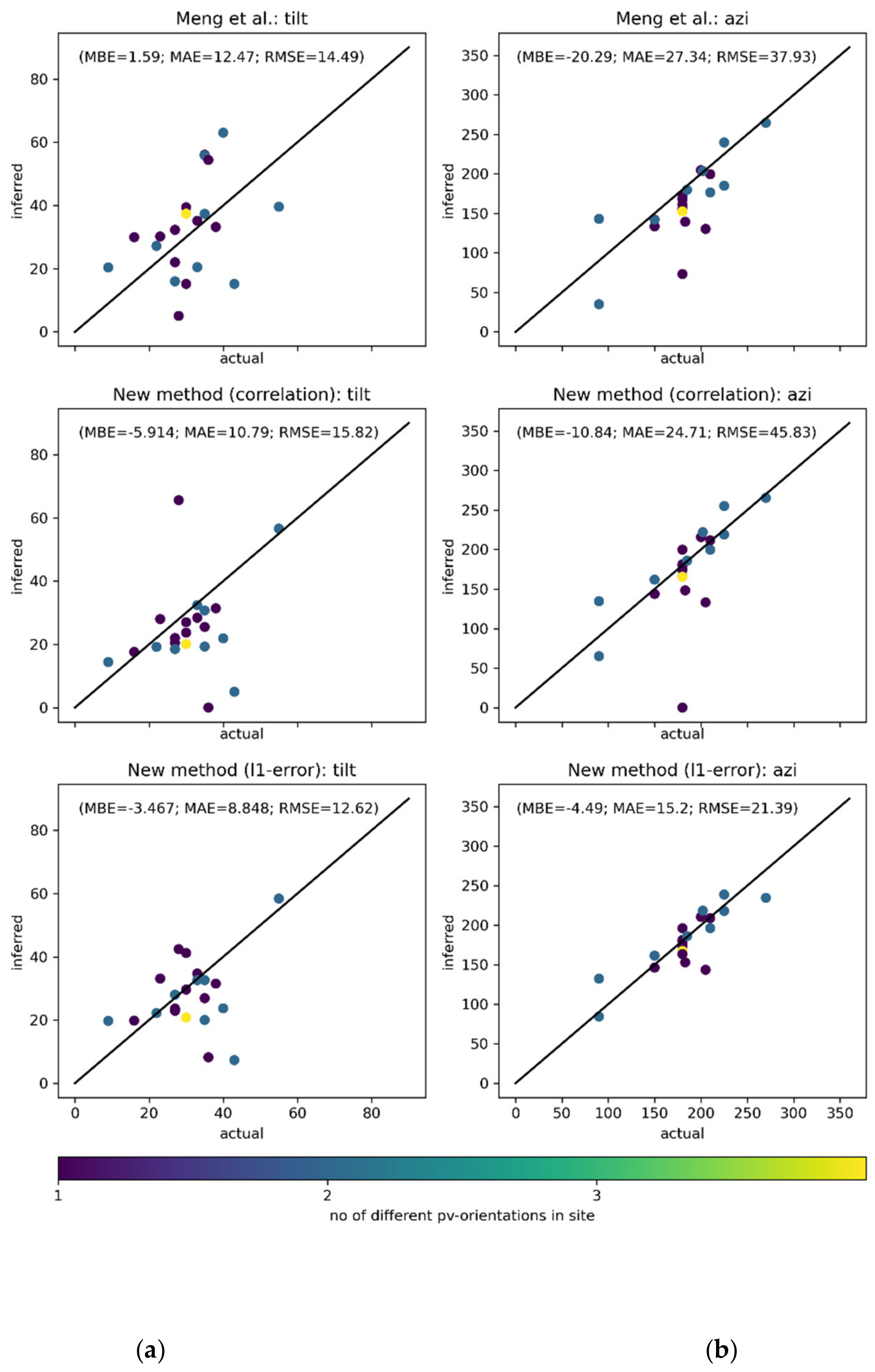
3.2. Inference of PV Array Tilt and Azimuth

The tilt and azimuth were estimated for the reference sites and those of the quality-controlled survey sites for which we had information about the geometry from the survey (n = 24). Scatterplots showing the reported and estimated tilts and azimuths are shown in Figure 4a,b for all three methods tested.

Summarizing the error statistics, we found the new method, optimizing the absolute error (l1-error) to be the most satisfactory. The plot includes sites with multiple orientations. If only sites with a single orientation are considered the bias, standard deviation and correlation coefficient are found to be −4°, 9°, and 0.3 for the tilt, and −6°, 10°, and 0.9 for the azimuth, respectively. The cause of the two outliers in the tilt estimation has not been investigated. Even if an error of about 10° may seem high, it did not have any major effect on the estimation of the clear sky model, as shown below.

3.3. Inference of Snow-Free Models

Using tilt and azimuth angles from the previous step, the shading coefficients were then estimated for all the quality-controlled basic and survey sites (n = 258), using the method described earlier. Error statistics for production during the same hours used for estimation (no snow in UERRA data and recorded production above its 5th percentile) are presented in

Table 3. Mean hourly error statistics for the snow-free models normalized with installed effect.

	Basic Sites (Estimated Tilt and Azimuth)	Survey Sites (Estimated Tilt and Azimuth)	Survey Sites (Recorded Tilt and Azimuth)
Number of sites	239	19	19
Pearson correlation	0.96	0.95	0.95
Bias (model—observation)	0.12%	0.022%	0.020%
Standard deviation	6.1%	6.9%	6.9%

. In the same table, we also give the error statistics separately for the sites where data about the panel geometry were known and used as input for the estimation of the snow-free models.

Note that there is no difference in performance between the snow-free models with respect to what information is used regarding the panel tilts and azimuths. Hence, we conclude that the quality of the estimated angles is good enough for use as input to the subsequent estimation of the snow-free model parameters. A density plot for the hourly snow-free production at all the 258 basic and survey sites (n = 2,004,830) is presented in Figure 5a.

3.4. Snow Loss Estimation

The snow loss was calculated as the difference between modeled snow-free production and measured production. Missing data were handled by requiring at least 90% data coverage during the daytime in order to obtain representable monthly values.

An example showing the estimated snow-free and actual monthly production at one of the basic sites is shown in Figure 5b. Note there are non-negligible snow losses during the winter 2017–2018 and that the 90% data-availability criteria caused a gap of two months in the graph during the start of 2019.

Moreover, note that there are some discrepancies between the model and the measurements, especially during the summer. The satellite data used in SARAH-2 are from the geostationary Meteosat satellite. Since these are located above the equator the view angle becomes large at northern latitudes, resulting in distorted cloud geometries. Moreover, we have so far only used an estimation of the direct component, derived from the global irradiance in SARAH-2 using the pvlib python function pvlib.irradiance.disc.

The choice to require at least valid data for measured PV yield for February, March, and April, in order to accept annual estimates is in line with the statistics for monthly contributions illustrated in the boxplot in Figure 6. The plot includes site-wise monthly means based on all years with at least 90% data availability per month. It shows that March is typically the month with the highest snow losses, responsible for 43% of all sites’ accumulated snow losses. February is clearly second in place, but the contributions for January and April are not that different in average contribution. April’s median value is lower than January’s, while its average value is higher. Since the higher values in the distribution for April are about twice as high as for January, it is reasonable to require data availability for this month—mostly April has not a very significant contribution, but in some cases, it is of such magnitude that it should not be ignored. The three months (February to April) together add up to a share of 79% overall (all sites and winters). Note that May contributions can be as high as January’s, larger than November or December. Snowfall in May is not so common but does occur. Early May there is also the possibility that snow from precipitation in April is still covering the PV array. In May, the amount of irradiation that is typically expected per hour of snow coverage is considerably higher than November–January. At the site with the highest latitude that is included in our study, the one hour with the highest global horizontal irradiation in May 2020 (819 Wh/m²) equaled almost half the irradiation during December 2018, the month with the lowest irradiation (1726 Wh/m²). Even though this example is somewhat extreme, it clearly indicates that very few hours of snow loss in May are enough to contribute more than months such as November or December.

Figure 7a shows the estimated snow losses for all sites that passed the quality checks, which are ordered by latitude to provide a sense of the geographic locations. Over time, new sites have been commissioned and added to the service providing the data, and therefore there are more blanks, i.e., missing data, in the earlier years.

To put the snow loss data into perspective, it can be compared to the mean specific yields in Figure 7b. The snow losses vary from 0–198 kWh/kWp. Yield for all sites and years varies between 356 kWh/kWp and 1262 kWh/kWp, with both the highest and lowest value situated near the same latitude. The reasons behind these extremities have not been investigated, but apart from physical causes, it might well be due to misreporting by the PV system owners. Either way, they are outliers compared to the median for all sites’ mean specific yields of 872 kWh/kWp and considering that 50% of all sites have a mean specific yield between 800 kWh/kWp and 956 kWh/kWp.

If we compare the three winter seasons with the most datapoints—2017/2018, 2018/2019, and 2019/2020—we notice that for basically all sites the first winter shows clearly higher snow losses than the second, which in turn has higher snow losses than the third winter. For the winter of 2017/2018, half of the sites have snow loss estimates between 28–71 kWh/kWp. Lower and upper quartiles for the specific yield for that same year were 734 kWh/kWp and 902 kWh/kWp, with a median of 819 kWh/kWp.

Relative annual snow losses are illustrated in the boxplot in Figure 8, showing values between 0% and 20%. For the snow-rich winter season of 2017/2018, the mean relative snow loss was 6.3%. It should be noted that snow conditions may vary considerably between sites, which might explain the large intervals. The lowest values could be impacted by site owners clearing the module array from time to time. We have not investigated the possibility of estimating this behavior but know from the survey sites that it is not very common (11% and 4% out of 85 contestants apply total clearance and clearing just the top layer of snow, respectively).

3.5. Comparison with Existing Snow Loss Models

Figure 9 below shows scatterplots for the comparison of snow loss estimations by our inference method and models by Marion et al, Ryberg and Freeman [10,16], and van Noord et al. [7]. The Marion model was applied twice, assuming either portrait or landscape module orientation. Since results were similar only the “portrait” results, which were slightly better, are presented in Figure 9.

The graph for the Marion model in Figure 9a clearly shows a correlation with the inferred model for annual snow-losses. The Pearson correlation coefficient between these models is 0.73. The bias and standard deviation for the Marion model estimates are −0.13 kWh/kWp (0.5% of mean annual snow losses) and 18 kWh/kWp (8.9% of mean), respectively. As discussed in the introduction section, monthly aggregate estimates of the Marion model typically show poorer correspondence, with large relative errors, and this is also true for our results.

The second model compared here, the lin–temp model, which assumes a linear relation between monthly average temperature and relative monthly snow loss, tends to overestimate the annual snow losses compared to the snow-free model. Interestingly, underestimation is very limited and stays at an almost equal distance of the 1:1-line slope. For this model comparison, the Pearson correlation is 0.66, somewhat lower than that for the Marion comparison. Bias and standard deviations are 17 kWh/kWp and 30 kWh/kWp, respectively, considerably higher than for the Marion model. Results for monthly estimates are in line with the annual results, i.e., higher bias and standard deviation than the Marion model estimates and relatively few numbers of underestimations (compared to our estimates).

3.6. Snow Loss and Panel Tilt Angle

Figure 10 shows the fractional snow loss (relative to the snow-free model) for March 2018, plotted as a function of panel tilt angle. For this month, there was snow covering almost all of Sweden, resulting in data from 161 sites. The data points are quite scattered, but after calculating the median loss for each 10-degree interval, one can see a trend in which the loss decreases with increasing tilt angle.

4. Discussion and Conclusions

The results show that the new approach presented in this article can be used to estimate snow losses with satisfying accuracy from just PV yield data and publicly available weather datasets. Snow losses for the included sites and years were estimated to vary from 0% to 20% of annual snow-free PV yield. Expressed in specific energy losses (energy normalized by installed DC-peak power) the estimates vary from 0 kWh/kWp to 198 kWh/kWp.

There is, on average, good agreement for the inferred PV yield model during snow-free hours, judging from high correlation (≥95%), low bias (<0.12%), and standard deviations (RMSE; 6–7%) as % of installed power. The latter is quite close to the 5% RMSE mentioned by Zamo et al [17] as the best performance in a benchmark of regression modeling methods—even considering they normalized in percent of maximum measured production. There, Zamo et al used ground-measured weather data from the nearest meteorological station rather than numerical weather models.

The inferred model’s performance for snow-free hours can be taken as an indicator that also the “snow-free” estimates for hours with snow cover are on average in good agreement. The model performance during hours with snow cover is however difficult to assess since we do not have measurements for snow-free PV systems to compare with. We did compare the snow loss estimates by the existing Marion model, and there is a pretty good correlation for annual values. Still, the Marion model’s estimates on a monthly basis show large deviations, similar to other studies [10,16]. There could, however, be several other explanations for these deviations. It can be an indication that the parameter values obtained for sites in the United States are not representative of the northern Swedish climate or the types of PV sites. It is also possible that uncertainties or errors in weather data (snow depth, temperature) are causing the deviations between the Marion model and our inferred model. Tilt estimate errors are less likely to explain the difference because the estimation method used tends to underestimate tilt angle, which would lead to higher estimates for the Marion model.

There are several parts of the approach presented in this article that allow for further improvement. Some main suggestions are discussed below.

The mean value for the estimated tilt angle in this study was about 25°. For this tilt angle, a 10° error will affect the snow-free POA irradiance during the snow season by about 5% (simulations with pvlib python using solar irradiance data from the SMHI radiation network). Improving the tilt angle estimate is, therefore, not critical for calculating the snow-free production, but it could be important for the estimation of snow losses and validation of existing prediction models. The Marion model uses the sine of the tilt angle in the estimation of the amount of snow slide. Here, the same 10-degree error as above translates into a difference of about 25%, regarding how fast the panel becomes snow-free. That 25% difference implies a significant impact on the expected loss in production. The fact that there is a relation between estimated loss and the tilt angle is illustrated in Figure 10. Thus, an improved tilt angle estimate could improve correlation with the Marion model. The same correlation might also benefit from a parameter fit for the Marion model to the inferred model’s results.

Moreover, there is room for improvement by extending the model to also detect cases with panels in multiple directions and infer multiple tilt angles.

It is possible that an improved tilt angle estimate can be obtained using our approach in combination with the direct irradiation from the SARAH-2 data instead of inferring it from the global irradiation using empirical methods as we did. Another way forward would be to look for alternative methods with a focus on obtaining good tilt estimates.

A better description of the direct irradiance could also help improve the snow-free model estimation, especially toward the summer when convection and patchy clouds affect the production to a greater extent. In Figure 5a, the density of the scatter of modeled and measured production during snow-free conditions looks convincing, but there are some caveats, and several sites were omitted during quality control. Improving the snow-free model should decrease the number of omitted sites and further increase statistics for snow loss studies using big-data.

Shading can be a real issue at some sites and should be investigated in more detail. Maybe one can find a good compromise when it comes to the time resolution of the shading factor for the direct component somewhere in-between an hourly and a monthly variation. Given that the amount of data available for analysis is sufficient.

Moreover, snow detection has room for improvement. Although snow detection by UERRA is conservative, it still misses out on a number of cases in which there is snow on the panels. Our simple comparison of satellite-based datasets of snow cover could possibly be extended with additional satellite products, reanalysis datasets, and other ways of processing the data. Furthermore, a combination of several data sources or processing methods could perhaps make the detection of snow-free cases more precise.

Several factors that are known or expected to impact snow clearance and/or snow losses still need more studying. We can mention ground or roof interference and the overall impact of module orientation—portrait versus landscape—on snow clearance and power losses. The ability to infer module orientation or key interference parameters from PV production data would create new possibilities to study these topics with a big-data approach.

One more aspect where inference methods could be developed is for the detection of non-natural snow clearance, such as manual sweeping or melting. The ability to detect these cases helps to study their impact and further improve snow loss prediction models.

Finally, it would be interesting to evaluate the proposed method at sites with ground truth regarding the production loss, for instance, at locations with twin installations, where one is cleared from snow and the other is not.

Currently, our planned next step will be to try and estimate snow losses at any location without knowing the production and only through given reanalysis data and information about the tilt and azimuth of the installation. Given the results obtained, we now have the data needed for doing a regression on a general level. This regression would provide us with maps indicating potential snow losses given the site location and geometry. Replacing the reanalysis data with climate projections would make it possible to study how snow losses may change in the future.

References

1. Masson, G.; Kaizuka, I. Trends in Photovoltaic Applications 2020; IEA PVPS, International Energy Agency: Paris, France, 2020. [Google Scholar]
2. Hashemi, B.; Cretu, A.-M.; Taheri, S. Snow Loss Prediction for Photovoltaic Farms Using Computational Intelligence Techniques. IEEE J. Photovoltaics 2020, 10, 1044–1052. [Google Scholar] [CrossRef]
3. Pawluk, R.E.; Chen, Y.; She, Y. Photovoltaic electricity generation loss due to snow—A literature review on influence factors, estimation, and mitigation. Renew. Sustain. Energy Rev. 2019, 107, 171–182. [Google Scholar] [CrossRef]
4. Powers, L.; Newmiller, J.; Townsend, T. Measuring and modeling the effect of snow on photovoltaic system performance. In Proceedings of the 2010 35th IEEE Photovoltaic Specialists Conference, Honolulu, HI, USA, 20–25 June 2010; IEEE: New York, NY, USA, 2010; pp. 973–978. [Google Scholar]
5. Heidari, N.; Gwamuri, J.; Townsend, T.; Pearce, J.M. Impact of Snow and Ground Interference on Photovoltaic Electric System Performance. IEEE J. Photovoltaics 2015, 5, 1680–1685. [Google Scholar] [CrossRef] [Green Version]
6. Townsend, T.; Powers, L. Photovoltaics and snow: An update from two winters of measurements in the SIERRA. In Proceedings of the 2011 37th IEEE Photovoltaic Specialists Conference, Seattle, WA, USA, 19–24 June 2011; IEEE: New York, NY, USA, 2011; pp. 3231–3236. [Google Scholar]
7. Van Noord, M.; Murphy, M.; Berglund, T. Investigating a Potential Linear Model for Prediction of Monthly Snow-Induced Production Losses for Rooftop PV. In Proceedings of the 33rd European Photovoltaic Solar Energy Conference Exhibition, Amsterdam, The Netherlands, 25–29 September 2017; pp. 2316–2319. [Google Scholar]
8. Sugiura, T.; Yamada, T.; Nakamura, H.; Umeya, M.; Sakuta, K.; Kurokawa, K. Measurements, analyses and evaluation of residential PV systems by Japanese monitoring program. Sol. Energy Mater. Sol. Cells 2003, 75, 767–779. [Google Scholar] [CrossRef]
9. Andrews, R.W.; Pollard, A.; Pearce, J.M. The effects of snowfall on solar photovoltaic performance. Sol. Energy 2013, 92, 84–97. [Google Scholar] [CrossRef] [Green Version]
10. Marion, B.; Schaefer, R.; Caine, H.; Sanchez, G. Measured and modeled photovoltaic system energy losses from snow for Colorado and Wisconsin locations. Sol. Energy 2013, 97, 112–121. [Google Scholar] [CrossRef]
11. Ross, M.M.D. Snow and Ice Accumulation on Photovoltaic Arrays: An Assessment of the TN Conseil Passive Melting Technology; Energy Diversification Research Laboratory, CANMET, Natural Resources Canada: Varennes, QC, Canada, 1995; p. 273. [Google Scholar]
12. Andenæs, E.; Jelle, B.P.; Ramlo, K.; Kolås, T.; Selj, J.; Foss, S.E. The influence of snow and ice coverage on the energy generation from photovoltaic solar cells. Sol. Energy 2018, 159, 318–328. [Google Scholar] [CrossRef]
13. van Noord, M.; Berglund, T.; Murphy, M. Snöpåverkan på Solelproduktion—Om Snöförluster på Takanläggningar i Norra Sverige; Energiforsk: Stockholm, Sweden, 2017; ISBN 978-91-7673-382-0. [Google Scholar]
14. Burnham, L.; Riley, D.; Braid, J. Design Considerations for Photovoltaic Systems Deployed in Snowy Climates. In Proceedings of the 37th European Photovoltaic Solar Energy Conference Exhibition, Online Event, 7–11 September 2020; pp. 1626–1631. [Google Scholar]
15. Hong, T.; Koo, C.; Lee, M. Estimating the Loss Ratio of Solar Photovoltaic Electricity Generation through Stochastic Analysis. J. Constr. Eng. Proj. Manag. 2013, 3, 23–34. [Google Scholar] [CrossRef] [Green Version]
16. Ryberg, D.; Freeman, J. Integration, Validation and Application of a PV Snow Coverage Model in SAM; National Renewable Energy Laboratory: Golden, CO, USA, 2015. [Google Scholar]
17. Zamo, M.; Mestre, O.; Arbogast, P.; Pannekoucke, O. A benchmark of statistical regression methods for short-term forecasting of photovoltaic electricity production, part I: Deterministic forecast of hourly production. Sol. Energy 2014, 105, 792–803. [Google Scholar] [CrossRef]
18. Shishavan, A.A.; Foresman, E.C.; Toor, F. Performance analysis of crystalline silicon and amorphous silicon photovoltaic systems in Iowa: 2011 to 2014. In Proceedings of the 2016 IEEE 43rd Photovoltaic Specialists Conference (PVSC), Portland, OR, USA, 5–10 June 2016; IEEE: New York, NY, USA, 2016; pp. 2625–2630. [Google Scholar]
19. Lorenz, E.; Heinemann, D.; Kurz, C. Local and regional photovoltaic power prediction for large scale grid integration: Assessment of a new algorithm for snow detection. Prog. Photovolt. Res. Appl. 2011, 20, 760–769. [Google Scholar] [CrossRef]
20. Bosman, L.; Darling, S. Difficulties and recommendations for more accurately predicting the performance of solar energy systems during the snow season. In Proceedings of the 2016 IEEE International Conference on Renewable Energy Research and Applications (ICRERA), Birmingham, UK, 20–23 November 2016; IEEE: New York, NY, USA, 2016; pp. 567–571. [Google Scholar]
21. Rahmatmand, A.; Harrison, S.J.; Oosthuizen, P.H. An Improved Numerical Method for Predicting Snow Melting on Photovoltaic Panels; IBPSA: Toronto, ON, Canada, 2016; p. 11. [Google Scholar]
22. National Renewable Energy Laboratory. System Advisor Model; National Renewable Energy Laboratory: Golden, CO, USA, 2020. [Google Scholar]
23. Pfeifroth, U.; Kothe, S.; Trentmann, J.; Hollmann, R.; Fuchs, P.; Kaiser, J.; Werscheck, M. Surface Radiation Data Set—Heliosat (SARAH-2)—Edition 2.1; CM SAF: Offenbach, Germany, 2019. [Google Scholar]
24. Eumetsat CM SAF. Available online: https://www.cmsaf.eu/ (accessed on 28 February 2021).
25. Unden, P.; Schimanke, S.; Le Moigne, P.; Bazile, E.; Ridal, M.; Olsson, E.; Berggren, L.; Randriamampianina, R. European High Resolution Regional Reanalyses in UERRA and the Copernicus Climate Change Service (C3S). In EMS Annual Meeting Abstracts; EMS: Berlin, Germany, 2018; Volume 15. [Google Scholar]
26. ECMWF. Complete UERRA Regional Reanalysis for Europe from 1961 to 2019. Available online: https://cds.climate.copernicus.eu/portfolio/dataset/reanalysis-uerra-europe-complete (accessed on 2 February 2021).
27. ECMWF. About Our Forecasts—Operational Configurations of the ECMWF Integrated Forecasting System (IFS). Available online: https://www.ecmwf.int/en/forecasts/documentation-and-support (accessed on 2 February 2021).
28. Landelius, T.; Josefsson, W.; Persson, T. Operational Mesoscale Radiation Modelling. In IRS 2000: Current Problems in Atmospheric Radiation; Smith, W.L., Timofeyev, Y.M., Eds.; Deepak Publishing: Hampton, VA, USA, 2001; pp. 66–69. [Google Scholar]
29. Trigo, I.F.; Dacamara, C.C.; Viterbo, P.; Roujean, J.-L.; Olesen, F.; Barroso, C.; Camacho-De-Coca, F.; Carrer, D.; Freitas, S.C.; García-Haro, J.; et al. The Satellite Application Facility for Land Surface Analysis. Int. J. Remote. Sens. 2011, 32, 2725–2744. [Google Scholar] [CrossRef]
30. Salomonson, V.; Appel, I. Development of the Aqua MODIS NDSI fractional snow cover algorithm and validation results. IEEE Trans. Geosci. Remote. Sens. 2006, 44, 1747–1756. [Google Scholar] [CrossRef]
31. CryoLand—The GMES Service for Snow and Land Ice. Available online: http://neso1.cryoland.enveo.at/ (accessed on 2 February 2021).
32. Nespoli, L.; Medici, V. An unsupervised method for estimating the global horizontal irradiance from photovoltaic power measurements. Sol. Energy 2017, 158, 701–710. [Google Scholar] [CrossRef] [Green Version]
33. Meng, B.; Loonen, R.; Hensen, J. Data-driven inference of unknown tilt and azimuth of distributed PV systems. Sol. Energy 2020, 211, 418–432. [Google Scholar] [CrossRef]
34. Holmgren, W.F.; Hansen, C.W.; Mikofski, M.A. pvlib python: A python package for modeling solar energy systems. J. Open Source Softw. 2018, 3, 884. [Google Scholar] [CrossRef] [Green Version]
35. Holmgren, W.; Hansen, C.; Mikofski, M.; Lorenzo, T.; Krien, U.; Stark, C.; Driesse, A.; de Leon Peque, M.S.; Miller, E.; Anoma, M.A.; et al. Pvlib/Pvlib-Python, V0.8.0; Zenodo: Genève, Switzerland, 2020. [Google Scholar]
36. Stack Overflow.Evenly Distributing n Points on a Sphere. Available online: stackoverflow.com (accessed on 2 February 2021).
37. Duffie, J.A.; Beckman, W.A.; Worek, W.M. Solar Engineering of Thermal Processes, 2nd ed. J. Sol. Energy Eng. 1994, 116, 67–68. [Google Scholar] [CrossRef]
38. Nuttall, A.H. Some windows with very good sidelobe behavior. IEEE Trans. Acoust. Speech, Signal Process. 1981, 29, 84–91. [Google Scholar] [CrossRef] [Green Version]
39. Tange, O. Gnu Parallel 2018; Zenodo: Genève, Switzerland, 2018. [Google Scholar]
Figure 1. Map of Sweden and surroundings showing site locations and data scope. Reference sites are marked with green dots (earlier study) and teal circles (current study), while survey and basic sites are marked with red dots.
Energies 14 01574 g001
Figure 2. An example of the dynamic evolution of the shading coefficient for the direct component throughout the year (thick blue line). Six fix shading coefficients (black dots), distributed symmetrically around the winter/summer solstice, were interpolated to any time of the year using the six corresponding Hann weighting functions (thin colored lines).
Energies 14 01574 g002
Figure 3. Histograms on the characteristics of the survey sites: (a) the number of module rows in the PV array height and (b) the orientation of the modules in the PV array.
Energies 14 01574 g003
Figure 4. Results from the estimation of panel geometries for different methods: (a) tilt and (b) azimuth.
Energies 14 01574 g004
Figure 5. Illustration of the performance of the inferred snow-free model: (a) density plot for measured and modeled hourly snow-free production normalized with the installed effect and (b) example of monthly modeled snow-free and actual observed production at one of the basic sites.
Energies 14 01574 g005
Figure 6. Boxplot for the mean of monthly contributions to the annual snow losses. Means are calculated for the sites with full winter season data (n = 257) and on average two winters (n = 542), with at least 90% data availability. Statistics presented in the plot are the median (green line), 50% (box), and 95% (whiskers) intervals as well as outliers (circles).
Energies 14 01574 g006
Figure 7. Results of normalized snow loss calculations in relation to the measured annual electricity yield for all quality-passed sites. The sites’ relative positions illustrate their geographical order by latitude: (a) estimated snow losses for the months September–May and years 2014–2020 and (b) annual mean yield for all years (June–May) with at least 90% data availability. Normalization for both graphs is by installed peak power (direct current at Standard Test Conditions—DC, STC).
Energies 14 01574 g007
Figure 8. Boxplot for percentual snow losses per winter season for all 258 sites. The figure indicates mean (red star), median (green line), 50% (box), 95% (whiskers) intervals, and outliers (circles).
Energies 14 01574 g008
Figure 9. Scatterplots for estimated winter season snow losses (September-May for 2014–2020) from the inference method described in this article and two existing snow loss models (energy losses normalized by installed peak power (DC, STC)): (a) Marion model [10], assuming arrays with unknown module mounting to have three rows of portrait-mounted modules. A single outlier point is left out and (b) lin–temp model [7].
Energies 14 01574 g009
Figure 10. Snow loss during March 2018 as a function of panel tilt angle. Blue dots indicate losses for each of 161 individual sites as a fraction of the modeled snow-free production. The orange line shows the median value for each 10-degree interval.
Energies 14 01574 g010