Analysis of Transient Interactions between a PWR Nuclear Power Plant and a Faulted Electricity Grid

Abstract

This paper presents the transient stability analysis of a pressurised water-type nuclear power plant following faults and disturbances affecting the electricity grid to which it is connected. The modelled nuclear plant consists of various integrated subsystems, such as core neutronics and thermal-hydraulics, piping and plenum, pressuriser, steam generator, turbine, governor, and dynamics shaft, in addition to the turbine-speed controller. The nonlinear nuclear power plant model is linearised at the operating point to acquire a linear model for controller design. The turbine-speed control loop effectively enacts a closed-loop implementation of the nuclear power plant connected to the electric grid. The various transient stability enhancement components such as the power system stabiliser, static var compensator, and static synchronous compensator are employed to test performance during severe contingencies. The interaction between the nuclear power plant, electric grid, and protection system is studied under various scenarios such as single-phase fault, three-phase fault, and permanent load loss. The performance of the nonlinear plant is further observed during load-following operation. The dynamic behaviour of the overall system is analysed using simulations in the MATLAB/Simulink/Simscape environment.

1. Introduction

Over the last few decades, the dependence on low carbon sources of energy such as nuclear power has grown remarkably. Due to the exigency of carbon-neutral electricity production, it is further expected to grow in the near future. Nuclear power plants are complex systems, generally having large capacities and high safety requirements. The coordination among plants, electric grids, protection systems, and utilities has advanced the operation of nuclear plants in a reserve capacity. The ever-increasing demand and new interconnections make the overall system vulnerable to faults, frequent plant trips, or even blackouts. Uncertainties and disturbances in the electric systems can seriously affect the nuclear power plant, grid, and interconnections. Large disturbances at the grid may cause a wide imbalance between demand and supply and can lead to excursions in the system voltage and frequency. As experienced in the North American blackout on 14 August 2003, such grid disturbances may induce significant transients in nuclear power plants connected to the faulted grid. It resulted, for instance, in large load adjustments, bypass of steam from the turbine generator, the opening of relief valves, and automatic startup of backup generators due to low voltages, all of which led to tripping the affected nuclear power plants [1]. Therefore, to ensure the safety and stability of nuclear plants and associated power systems, it is essential to inspect the effects of grid disturbances on nuclear power plants.

The transient analysis of interactions among different systems has been considered by a few studies in nuclear engineering literature. In the earliest works [2,3,4], the protection of nuclear power plants has been discussed; however, the mutual influences between the nuclear power plants, grid, and their protection systems have not been sufficiently considered. The conventional models of nuclear power plants proposed therein have high computational complexities, which further limited their suitability in large-scale power system dynamic simulations. Linear nuclear power plant models have been employed for short-term stability investigation of the power system for a slow and small range of output variations [5,6,7,8,9,10,11,12,13]. In these works, the subsystems are given by simplified dynamic equations, which make them preferable in short-term dynamic analysis during small power imbalance conditions. They assume that the excursions in power system frequency and voltage are due to small system disturbances. Thus, the models are not sufficient for long-term dynamics analysis and are inadequate in the case of large disturbances. Moreover, they do not represent the detailed dynamics of a nuclear power plant.

In some recent works [14,15,16,17], empirical formulation-based and first principles-based models have been proposed for power system analysis. An optimisation-based method has been put forward by Wang et al. for power systems analysis in advanced pressurised water reactor (PWR) [14]. Wu et al. studied the frequency and voltage excursions and discussed the coordinated control and protection of nuclear power plants and grids [15]. For the over-frequency protection of nuclear power plants, a speed-governing system model was also proposed [16]. Lately, a model for a small modular reactor was suggested to study the power system dynamics [17]. Most of the reported work on nuclear power plant modelling for power system analysis represents only some specific subsystem of the plant. In addition, most of the studies have combined a simplified nuclear plant model with a power system model. A detailed analysis of the integrated nuclear plant model connected with an electric grid is not rigorously carried out using the available power system simulation software packages. The detailed response of plant and network variables have also not been performed in the abovementioned literature as is done in this manuscript. Nonetheless, a complete yet simple integrated nuclear power plant model is required for use in transient analysis, control systems design, and evaluation of the system’s response following short-circuits affecting the grid or large and sudden fluctuations in demand.

The interconnection of power systems is beneficial when increasing the reliability of the system and when minimising the operational costs through resource sharing. To improve the overall performance under detrimental situations and to fulfil the comprehensive reliability demands, transient analysis of a detailed nuclear power plant–grid integrated model is required. Based on operational experience, the international atomic energy agency has put forward the characteristics, interactions, and compatibility of nuclear power plants with grids of limited capacity [18]. A reliability study of transmission grids and nuclear power plants during voltage excursions in a transmission system has been studied by Kirby et al. [19]. During electrical disturbances or small interruptions in the power network, the interconnection of nuclear power plants, power systems, and transmission lines makes the overall system susceptible to low-frequency electromechanical oscillations. These oscillations can affect the transient stability of the power system by inducing fluctuations in the line frequency and currents, bus voltages, and generator speeds. The transient stability is further affected by overloading transmission lines due to increased power demands. A power system stabiliser (PSS) is usually employed with the excitation system to maintain synchronism and power flow and to enlarge power transfer limits. The PSS enhances damping during weak transmission situations, accompanying hefty load transfer by modifying the torque angle of the shaft. PSS has been employed to analyse the consequence of a severe power grid fault on the generator of Million Kilowatts nuclear power plant [20]. However, the PSS alone cannot damp oscillations under extreme grid disturbances, and its effectiveness is limited to small excursions around a steady-state point for a nonlinear system [21,22]. Hence, it is essential to advance computationally intelligent controllers for accurate and faster control action.

Flexible alternating current transmission systems (FACTS) are widely employed to stabilise the transmission system. They regulate the network conditions with optimal speed to boost the power transfer capability. FACTS devices increase the controllability and strengthen the steady-state and transient stabilities. During transient oscillations, the frequency and voltage control loops regulate the system frequency and voltage to maintain synchronism. Static var compensator (SVC) and static synchronous compensator (STATCOM) are two widely employed shunt-type FACTS devices. The SVC is based on thyristors valves. It regulates the reactive power absorbed from or injected into the power system to control the voltage at its terminals. STATCOM is a voltage-source converter-based device that can act either as a source or as a sink for reactive power to an electricity network. Both power electronics devices work to reduce voltage fluctuations. Moreover, the coordinated action of PSS and SVC, or PSS and STATCOM provides useful means to enhance stability.

The proposed work analyses the transient stability of a PWR-type nuclear power plant connected to an electric grid in the presence of faults and disturbances. The employed model of a PWR-type plant consists of various integrated subsystems, such as core neutronics, thermal hydraulics, piping and plenum, pressuriser, steam generator, turbine, governor, turbine-speed controller, dynamics shaft, actuators, and sensors. This model can be interfaced with a power grid model to enable the study of the dynamic interactions between the grid and the nuclear power plant. To the best of the authors’ knowledge, there is no detailed work available in the nuclear energy literature on the systematic incorporation of transient stability enhancement devices in a complete nuclear plant–electric grid model. In this paper, generic PSS and multi-band PSS are connected with SVC and STATCOM to analyse the transient stability of the PWR-type plant connected to the grid in the presence of multiple single-phase faults, multiple three-phase faults, and permanent load loss situations. The dynamic response of the system is discussed using plant and power system variables. The simulations are performed under the MATLAB/Simulink/Simscape environment.

The rest of the paper is organised as follows: Section 2 presents the complete dynamical model of a PWR-type plant. Section 3 presents different transient stability enhancement components. Section 4 discusses the interconnection and coordination of a nuclear power plant with the grid. Section 5 discusses the simulation results. Finally, conclusions are drawn in Section 6.

2. Mathematical Model of a PWR Nuclear Power Plant

A simple interconnection of the modelled PWR-type nuclear power plant connected to the electric grid is shown in Figure 1. The various subsystems of the integrated model have been considered in depth in [16,23,24,25]. The integrated model has been analysed and verified with simulated as well as plant data in [26]. In this work, a dynamic shaft model has been further incorporated in the integrated model [27]. To avoid duplication of published work, the PWR-type nuclear power plant model is presented here in brief. For a detailed description, the readers are advised to refer to [26,28,29]. The values of plant parameters, steady-state values, and their detailed definitions are given in [26,28,29].

2.1. Core Neutronics Model

2.1.1. Reactor Point Kinetics

The reactor point kinetics model consists of power ($P_n$) and precursor concentration of six groups of delayed neutrons ($C_{in}$). They are normalised by their steady state values and are defined as

$$\begin{array}{ccc}\hfill \frac{d{P}_n}{dt}& =& \frac{{\rho }_t-{\displaystyle \sum _{i=1}^6}{\beta }_i}{\Lambda }{P}_n+{\displaystyle \sum _{i=1}^6}\frac{{\beta }_i}{\Lambda }{C}_{in}\hfill \end{array}$$

(1)

$$\begin{array}{ccc}\hfill \frac{d{C}_{in}}{dt}& =& {\lambda }_i{P}_n-{\lambda }_i{C}_{in},i=1,2,\dots 6\hfill \end{array}$$

(2)

where $\Lambda$ is neutron generation time. ${\beta }_i$ and ${\lambda }_i$ are the fraction of delayed neutrons and decay constant of the ith group, respectively.

2.1.2. Ex-Core Detectors

The reactor power can be sensed using ex-core detectors. The ex-core detectors produce an ex-core detector current ($i_{lo}$) proportional to the neutronic power, which is amplified by a logarithmic amplifier as follows [30]:

$${\tau }_1{\tau }_2\frac{d^2{i}_{lo}}{d{t}^2}+\left({\tau }_1+{\tau }_2\right)\frac{d{i}_{lo}}{dt}+i_{lo}=K_{lo}{log}_{10}\left({\kappa }_{lo}{P}_n\right)$$

(3)

where ${\kappa }_{lo}$ is a constant. $K_{lo}$ is the logarithmic amplifier gain. ${\tau }_1$ and ${\tau }_2$ are logarithmic amplifier time constants.

2.1.3. Reactivity Feedback

The reactivity model incorporates reactivity due to the rod movement and feedback because of the impact of variation in the temperature and pressure of fuel and coolant. The total reactivity ${\rho }_t$ is stated as follows:

$$\begin{array}{c}\hfill \begin{array}{c}{\rho }_t={\rho }_{rod}+{\alpha }_f{T}_f+{\alpha }_c{T}_{c1}+{\alpha }_c{T}_{c2}+{\alpha }_p{p}_p\hfill \end{array}\end{array}$$

(4)

where the reactivity due to control the rod (${\rho }_{rod}$) is governed by the rod speed ($v_{rod}$) and the rod worth (G) and is given by

$$\frac{d{\rho }_{rod}}{dt}=G{v}_{rod}$$

(5)

where ${\alpha }_f$, ${\alpha }_c$, and ${\alpha }_p$ are reactivity coefficients because of feedback from fuel and coolant temperatures and pressuriser pressure.

2.2. Thermal-Hydraulics Model

2.2.1. Fuel-Coolant Node

The core thermal-hydraulics behaviour is determined by Mann’s model [23], which correlates the neutronic power to the temperatures of fuel ($T_f$) to coolant nodes ($T_{c1}$ and $T_{c2}$) as follows:

$$\begin{array}{ccc}\hfill \frac{d{T}_f}{dt}& =& H_f{P}_n-\frac{1}{{\tau }_f}\left(T_f-T_{c1}\right)\hfill \end{array}$$

(6)

$$\begin{array}{ccc}\hfill \frac{d{T}_{c1}}{dt}& =& H_c{P}_n-\frac{2}{{\tau }_r}\left(T_{c1}-T_{cin}\right)+\frac{1}{{\tau }_c}\left(T_f-T_{c1}\right)\hfill \end{array}$$

(7)

$$\begin{array}{ccc}\hfill \frac{d{T}_{c2}}{dt}& =& H_c{P}_n-\frac{2}{{\tau }_r}\left(T_{c2}-T_{c1}\right)+\frac{1}{{\tau }_c}\left(T_f-T_{c1}\right)\hfill \end{array}$$

(8)

where ${\tau }_f$, ${\tau }_c$, and ${\tau }_r$ are time constants. $H_c$ and $H_f$ are the rate of rise of coolant and fuel temperatures, respectively.

2.2.2. Resistance Temperature Detectors

Resistance temperature detectors (RTD) are employed to sense the coolant temperature at the inlet ($T_{rtd1}$) and outlet ($T_{rtd2}$) and can be described as follows:

$$\frac{d{T}_{rtd1}}{dt}=\frac{1}{{\tau }_{rtd}}\left(-T_{rtd1}+2T_{c1}-T_{rxi}\right)$$

(9)

$$\frac{d{T}_{rtd2}}{dt}=\frac{1}{{\tau }_{rtd}}\left(-T_{rtd2}+2T_{c2}-T_{rxu}\right)$$

(10)

A current signal ($i_{rtd}$) can be acquired from the monitored RTD signals as follows: [30]

$$i_{rtd}=K_{rtd}\frac{\left(\left(\left(T_{rtd1}+T_{rtd2}\right)/\phantom{\left(T_{rtd1}+T_{rtd2}\right)2}2\right)-T_{rxi0}\right)}{\left(T_{rxu0}-T_{rxi0}\right)}+4$$

(11)

where $K_{rtd}$ and ${\tau }_{rtd}$ are the gain and time constant of RTD, respectively.

2.3. Piping and Plenum Model

Hot-leg piping ($T_{hot}$), cold-leg piping ($T_{cold}$), reactor lower-plenum ($T_{rxi}$), reactor upper-plenum ($T_{rxu}$), steam generator inlet-plenum ($T_{sgi}$), and steam generator outlet-plenum ($T_{sgu}$) can be represented as follows [23]:

$$\begin{array}{ccc}\hfill \frac{d{T}_{rxu}}{dt}& =& \frac{1}{{\tau }_{rxu}}\left(T_{c2}-T_{rxu}\right)\hfill \end{array}$$

(12)

$$\begin{array}{ccc}\hfill \frac{d{T}_{hot}}{dt}& =& \frac{1}{{\tau }_{hot}}\left(T_{rxu}-T_{hot}\right)\hfill \end{array}$$

(13)

$$\begin{array}{ccc}\hfill \frac{d{T}_{sgi}}{dt}& =& \frac{1}{{\tau }_{sgi}}\left(T_{hot}-T_{sgi}\right)\hfill \end{array}$$

(14)

$$\begin{array}{ccc}\hfill \frac{d{T}_{sgu}}{dt}& =& \frac{1}{{\tau }_{sgu}}\left(T_{p2}-T_{sgu}\right)\hfill \end{array}$$

(15)

$$\begin{array}{ccc}\hfill \frac{d{T}_{cold}}{dt}& =& \frac{1}{{\tau }_{cold}}\left(T_{sgu}-T_{cold}\right)\hfill \end{array}$$

(16)

$$\begin{array}{ccc}\hfill \frac{d{T}_{rxi}}{dt}& =& \frac{1}{{\tau }_{rxi}}\left(T_{cold}-T_{rxi}\right)\hfill \end{array}$$

(17)

where ${\tau }_{rxu}$, ${\tau }_{rxi}$, ${\tau }_{hot}$, ${\tau }_{cold}$, ${\tau }_{sgu}$, and ${\tau }_{sgi}$ denote time constants.

2.4. Steam Generator Model

A five-node model can suitably describe the steam-generator (SG), in which the primary coolant node (PCL) ($T_{p1}$ and $T_{p2}$) and metal tube node (MTL) ($T_{m1}$ and $T_{m2}$) are given by two nodes each and the secondary coolant node (SCL) is given by one node [24]. It is given as follows:

$$\begin{array}{ccc}\hfill \frac{d{T}_{p1}}{dt}& =& \frac{1}{{\tau }_{p1}}\left(T_{sgi}-T_{p1}\right)-\frac{1}{{\tau }_{pm1}}\left(T_{p1}-T_{m1}\right)\hfill \end{array}$$

(18)

$$\begin{array}{ccc}\hfill \frac{d{T}_{p2}}{dt}& =& \frac{1}{{\tau }_{p2}}\left(T_{p1}-T_{p2}\right)-\frac{1}{{\tau }_{pm2}}\left(T_{p2}-T_{m2}\right)\hfill \end{array}$$

(19)

$$\begin{array}{ccc}\hfill \frac{d{T}_{m1}}{dt}& =& \frac{1}{{\tau }_{mp1}}\left(T_{p1}-T_{m1}\right)-\frac{1}{{\tau }_{ms1}}\left(T_{m1}-T_s\right)\hfill \end{array}$$

(20)

$$\begin{array}{ccc}\hfill \frac{d{T}_{m2}}{dt}& =& \frac{1}{{\tau }_{mp2}}\left(T_{p2}-T_{m2}\right)-\frac{1}{{\tau }_{ms2}}\left(T_{m2}-T_s\right)\hfill \end{array}$$

(21)

where ${\tau }_{p1}$, ${\tau }_{p2}$, ${\tau }_{pm1}$, ${\tau }_{pm2}$, ${\tau }_{mp1}$, ${\tau }_{mp2}$, ${\tau }_{ms1}$, and ${\tau }_{ms2}$ denote the time constants. SCL represents the steam pressure ($p_s$) as follows:

$$\frac{d{p}_s}{dt}=\frac{1}{K_s}\left[U_{ms1}{S}_{ms1}\left(T_{m1}-T_s\right)+U_{ms2}{S}_{ms2}\left(T_{m2}-T_s\right)-\left({\dot{m}}_{so}{h}_{ss}-{\dot{m}}_{fw}{c}_{pfw}{T}_{fw}\right)\right]$$

(22)

where $S_{ms1}$ and $U_{ms1}$ are the effective heat transfer area and the heat transfer coefficient from MTL 1 to SCL, respectively. Similar definitions are valid for $S_{ms2}$ and $U_{ms2}$. $c_{pfw}$ is the specific heat of feed water. $T_{fw}$ is the temperature of feed water. ${\dot{m}}_{fw}$ and ${\dot{m}}_{so}$ denote the mass flow rate of feed water and steam, respectively. The constant $K_s$ is defined as follows:

$$K_s=m_{ws}\frac{\partial h_{ws}}{\partial p_s}+m_{ss}\frac{\partial h_{ss}}{\partial p_s}-m_{ws}\left(\frac{h_{ws}-h_{ss}}{{\nu }_{ws}-{\nu }_{ss}}\right)\frac{\partial {\nu }_{ss}}{\partial p_s}$$

(23)

where $m_{ws}$, $h_{ws}$, and ${\nu }_{ws}$ denote the mass, enthalpy, and specific volume of water in the secondary lump, respectively. Similarly, $m_{ss}$, $h_{ss}$, and ${\nu }_{ss}$ are the parameters for steam in the SCL.

2.5. Pressuriser Model

The pressuriser pressure ($p_p$) is given by balancing the volume and energy of water and steam mixture besides steam compressibility as follows [25]:

$$\frac{dp{}_p}{dt}=\frac{\begin{array}{c}{Q}_{heat}+{\dot{m}}_{sur}\left(\frac{p{}_p{\nu }_s}{J_p{C}_{1p}}+\frac{h_{\overline{w}}}{C_{1p}}\right)+{\dot{m}}_{spr}\left(h_{spr}-h_w+\frac{h_{\overline{w}}}{C_{1p}}+\frac{p{}_p{\nu }_w}{J_p{C}_{1p}}\right)\hfill \end{array}}{\begin{array}{c}{m}_w\left(K_{3p}+\frac{K_{4p}p{}_p}{J_p}\right)+\frac{m_s{K}_{4p}p{}_p}{J_p}-\frac{V_w}{J_p}+\frac{C_{2p}}{C_{1p}}\left(h_{\overline{w}}+\frac{p{}_p{\nu }_s}{J_p}\right)\hfill \end{array}}$$

(24)

where $Q_{heat}$ is rate of heat addition by heater, ${\dot{m}}_{spr}$ is mass spray flow rate, and ${\dot{m}}_{sur}$ is mass surge flow rate. $m_w$, $d_w$, $h_w$, and ${\nu }_w$ are mass, density, enthalpy, and specific volume of water. Similarly, $m_s$, $d_s$, and ${\nu }_s$ denote the parameters for steam. $h_{\overline{w}}$ and $h_{spr}$ are the latent heat of vaporisation and enthalpy of spray, respectively. $J_p$ is the conversion factor, and $V_w$ is water volume. The mass surge flow rate is given by the coolant temperatures at different nodes as follows:

$${\dot{m}}_{sur}={\displaystyle \sum _{j=1}^N}{V}_j{\vartheta }_j\frac{d{T}_j}{dt}$$

(25)

where $V_j$ is volume and ${\vartheta }_j$ is the slope of coolant density versus temperature curve for the jth node.

The equation of water level ($l_w$) in the pressuriser is derived by balancing the mass equations on water and steam phase as follows:

$$\frac{d{l}_w}{dt}=\frac{1}{d_s{A}_p}\left(\left(A_p\left(l-l_w\right)K_{2p}-\frac{C_{2p}}{C_{1p}}\right)\frac{dp{}_p}{dt}+\frac{1}{C_{1p}^2}\left(C_{2p}\frac{dp{}_p}{dt}-{\dot{m}}_{sur}-{\dot{m}}_{spr}\right)+\frac{{\dot{m}}_{sur}}{C_{1p}}\right)$$

(26)

where $A_p$ is the cross-sectional area and l is the length of the pressuriser. The other variables are defined as follows:

$$\begin{array}{ccc}\hfill C_{1p}& =& \frac{d_w}{d_s}-1;\hfill \end{array}$$

(27)

$$\begin{array}{ccc}\hfill C_{2p}& =& A_p\left(l-l_w\right)\frac{d_w}{d_s}{K}_{2p}+A_p{l}_w{K}_{1p};\hfill \end{array}$$

(28)

$$\begin{array}{ccc}\hfill K_{1p}& =& \frac{\partial d_w}{\partial p_p};K_{2p}=\frac{\partial d_s}{\partial p_p};K_{3p}=\frac{\partial h_w}{\partial p_p};K_{4p}=\frac{\partial {\nu }_s}{\partial p_p}.\hfill \end{array}$$

(29)

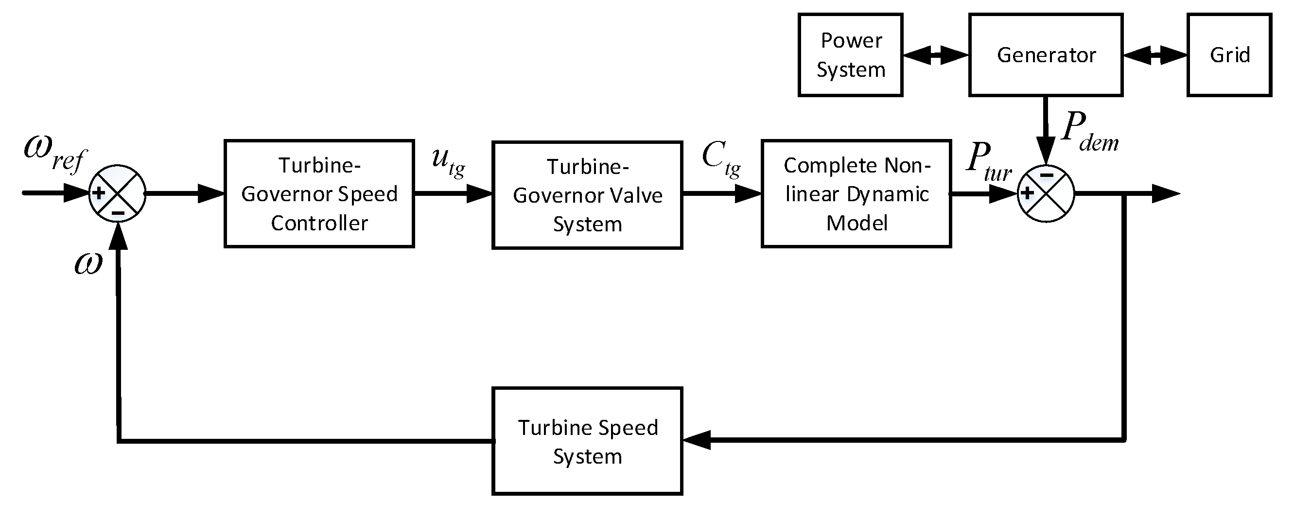
2.6. Turbine-Governor Model

2.6.1. Turbine

The turbine model is comprised of the high-pressure, intermediate-pressure, and low-pressure turbines. These are given by the following [16]:

$$\begin{array}{ccc}& & \frac{d^2{P}_{hp}}{dt}+\left(\frac{O_{rv}+{\tau }_{ip}}{{\tau }_{hp}{\tau }_{ip}}\right)\frac{d{P}_{hp}}{dt}+\frac{O_{rv}{P}_{hp}}{{\tau }_{hp}{\tau }_{ip}}=\frac{O_{rv}{F}_{hp}{\overline{\dot{m}}}_{so}}{{\tau }_{hp}{\tau }_{ip}}+\left(\frac{\left(1+{\kappa }_{hp}\right)F_{hp}}{{\tau }_{hp}}\right)\frac{d{\overline{\dot{m}}}_{so}}{dt}\hfill \end{array}$$

(30)

$$\begin{array}{ccc}& & \frac{d^2{P}_{ip}}{dt}+\left(\frac{O_{rv}{\tau }_{hp}+{\tau }_{ip}}{{\tau }_{hp}{\tau }_{ip}}\right)\frac{d{P}_{ip}}{dt}+\frac{O_{rv}{P}_{ip}}{{\tau }_{hp}{\tau }_{ip}}=\frac{O_{rv}{F}_{ip}{\overline{\dot{m}}}_{so}}{{\tau }_{hp}{\tau }_{ip}}\hfill \end{array}$$

(31)

$$\begin{array}{ccc}& & \frac{d^3{P}_{lp}}{dt}+\left(\frac{O_{rv}{\tau }_{hp}+{\tau }_{ip}}{{\tau }_{hp}{\tau }_{ip}}+\frac{1}{{\tau }_{lp}}\right)\frac{d^2{P}_{lp}}{dt}+\left(\frac{O_{rv}\left({\tau }_{lp}+{\tau }_{hp}\right)+{\tau }_{ip}}{{\tau }_{hp}{\tau }_{ip}{\tau }_{lp}}\right)\frac{d{P}_{lp}}{dt}+\frac{O_{rv}{P}_{lp}}{{\tau }_{hp}{\tau }_{ip}{\tau }_{lp}}=O_{rv}{F}_{lp}{\overline{\dot{m}}}_{so}\hfill \end{array}$$

(32)

where $O_{rv}$ is the valve opening degree. ${\kappa }_{hp}$ is high-pressure natural power overshooting coefficient. ${\tau }_{hp}$, $F_{hp}$, and $P_{hp}$ denote the volume time constant, fraction of steady-state power output, and mechanical power output of a high-pressure turbine, respectively. Similar definitions are valid for ${\tau }_{ip}$, $F_{ip}$, and $P_{ip}$ for the intermediate-pressure turbine and ${\tau }_{lp}$, $F_{lp}$, and $P_{lp}$ for the low-pressure turbine. The total mechanical output of turbine ($P_{tur}$) is computed as follows:

$$P_{tur}=P_{hp}+P_{ip}+P_{lp}$$

(33)

2.6.2. Turbine-Governor Valve

The steam flow rate is related to the turbine-governor control valve coefficient ($C_{tg}$) as follows:

$${\dot{m}}_{so}=C_{tg}{p}_s$$

(34)

where the steam flow is ${\overline{\dot{m}}}_{so}=\frac{{\dot{m}}_{so}}{{\dot{m}}_{sor}}$. The ${\dot{m}}_{sor}$ denotes the rated steam mass flow rate. The valve coefficient can be adjusted using the input signal ($u_{tg}$) as follows:

$$\frac{d^2{C}_{tg}}{d{t}^2}+2{\zeta }_{tg}{\varpi }_{tg}\frac{d{C}_{tg}}{dt}+{\varpi }_{tg}^2{C}_{tg}={\varpi }_{tg}^2{K}_{tg}{u}_{tg}$$

(35)

where ${\zeta }_{tg}$ is the damping ratio, ${\varpi }_{tg}$ is the natural frequency of oscillation, $K_{tg}$ is the gain in the turbine-governor valve.

2.7. Dynamic Shaft Model

The dynamic shaft model of a synchronous machine can be described by a dynamic mass-spring mode [27]. It contains low-, intermediate-, and high-pressure turbine masses; exciter mass; and machine rotor. The high-pressure turbine mass-spring model is given by the following:

$${\dot{\delta }}_{hp}={\Omega }_b\left({\omega }_{hp}-{\omega }_s\right)$$

(36)

$${\dot{\omega }}_{hp}=\frac{q_{tur}-D_{hp}\left({\omega }_{hp}-{\omega }_s\right)-D_{hi}\left({\omega }_{hp}-{\omega }_{ip}\right)+K_{hp}\left({\delta }_{ip}-{\delta }_{hp}\right)}{2H_{hp}}$$

(37)

where ${\Omega }_b$ is base synchronous frequency, ${\omega }_s$ is reference frequency, $q_{tur}$ is turbine torque related with turbine power as $P_{tur}=q_{tur}{\omega }_{tur}$, and $q_e$ is electric torque. ${\delta }_{hp}$ is rotor angle, ${\omega }_{hp}$ is frequency, D is the turbine damping coefficient, $K_{hp}$ is the angle coefficient, and $H_{hp}$ is the inertia constant for a high-pressure turbine. Similar definitions hold for an intermediate-pressure turbine, a low-pressure turbine, the machine rotor, and the exciter denoted by subscripts $ip$, $lp$, $mr$, and $ex$, respectively. The turbine dampings for high–intermediate, intermediate–low, low–rotor, and rotor–exciter are denoted as $D_{hi}$, $D_{il}$, $D_{lr}$, and $D_{re}$, respectively.

The intermediate-pressure turbine mass-spring model is given by the following:

$${\dot{\delta }}_{ip}={\Omega }_b\left({\omega }_{ip}-{\omega }_s\right)$$

(38)

$${\dot{\omega }}_{ip}=\frac{-D_{ip}\left({\omega }_{ip}-{\omega }_s\right)-D_{hi}\left({\omega }_{ip}-{\omega }_{hp}\right)-D_{il}\left({\omega }_{ip}-{\omega }_{lp}\right)+K_{hp}\left({\delta }_{hp}-{\delta }_{ip}\right)+K_{ip}\left({\delta }_{lp}-{\delta }_{ip}\right)}{2H_{ip}}$$

(39)

The low-pressure turbine mass-spring model is given by the following:

$${\dot{\delta }}_{lp}={\Omega }_b\left({\omega }_{lp}-{\omega }_s\right)$$

(40)

$${\dot{\omega }}_{lp}=\frac{-D_{lp}\left({\omega }_{lp}-{\omega }_s\right)-D_{il}\left({\omega }_{lp}-{\omega }_{ip}\right)-D_{lr}\left({\omega }_{lp}-{\omega }_{mr}\right)+K_{ip}\left({\delta }_{ip}-{\delta }_{lp}\right)+K_{lp}\left({\delta }_{mr}-{\delta }_{lp}\right)}{2H_{lp}}$$

(41)

The machine rotor mass-spring model is given by the following:

$${\dot{\delta }}_{mr}={\Omega }_b\left({\omega }_{mr}-1\right)$$

(42)

$${\dot{\omega }}_{mr}=\frac{-q_e-D_{mr}\left({\omega }_{mr}-{\omega }_s\right)-D_{lr}\left({\omega }_{mr}-{\omega }_{lp}\right)-D_{re}\left({\omega }_{mr}-{\omega }_{ex}\right)+K_{lp}\left({\delta }_{lp}-{\delta }_{mr}\right)+K_{ex}\left({\delta }_{ex}-{\delta }_{mr}\right)}{2H}$$

(43)

The exciter mass-spring model is given by the following:

$${\dot{\delta }}_{ex}={\Omega }_b\left({\omega }_{ex}-{\omega }_s\right)$$

(44)

$${\dot{\omega }}_{ex}=\frac{-D_{ex}\left({\omega }_{ex}-{\omega }_s\right)-D_{re}\left({\omega }_{ex}-\omega \right)+K_{ex}\left(\delta -{\delta }_{ex}\right)}{2H_{ex}}$$

(45)

2.8. Turbine-Speed Control Loop

The control loop structure of the turbine-speed system is depicted in Figure 2, in which the speed can be controlled using a turbine-governor valve. The valve regulates the steam flow to modify the speed [25,26]. The PI controller output of the configuration can be stated as follows:

$$u_{tg}=\left(K_{P,tg}+\frac{K_{I,tg}}{s}\right)\left({\omega }_{ref}-{\omega }_{mr}\right)$$

(46)

where $K_{P,tg}$ and $K_{I,tg}$ are the proportional and integral gain, respectively.

3. Transient Stability Enhancement Components

The transient stability of a system is given as its capability to maintain a stable condition after large disturbances [31]. Various methods are available to improve the transient stability of power systems, such as fast-acting exciters, power system stabilisers, and FACTS devices.

3.1. Automatic Voltage Regulator

The automatic voltage regulator (AVR) is a power system controller that is a part of the excitation system of the generator. It regulates the terminal voltage by modifying the exciter voltage, which in turn regulates the power factor of the machine as well as reactive power generation. The AVR tries to maintain the system voltage within the desired output in steady-state as well as in transient situation to make certain that the generator remains synchronised to the grid system after grid faults. It provides the lag sensitivity to vary the field voltage of the generator rapidly. Nevertheless, the usage of an AVR can prompt the retention of long-term low-frequency oscillation, and thus, this may affect power system equipment and it may reduce the system performance.

3.2. Power System Stabiliser

The power system stabiliser (PSS) is a vital tool to enhance overall system stability [32]. Its wide usage is due to its low cost and good performance over a broad span of operating conditions. The central purpose of a PSS is to alleviate any undamped power oscillations restricting the steady-state transfer capability. The working principle of a PSS is to generate an electrical torque in phase with the rotor speed deviations and to include damping to the generator rotor oscillations by regulating its excitation using stabilising signals. Here, two of the known variants (generic PSS and multiband PSS) are considered in the study.

3.2.1. Generic Power System Stabiliser

The generic PSS (GPSS) is comprised of a gain block, low-pass and high-pass filters, an output limiter, and a phase-compensation system [32]. The block diagram of a GPSS is depicted in Figure 3. The input to the GPSS is the speed deviation signal coming from the synchronous machine, which in turn is derived using the difference between the output of mechanical power and electrical power. The overall gain determines the damping torque by a GPSS. The low frequencies are eliminated using a wash-out high-pass filter for which the time constant should permit frequency shaping of the input. Generally, an inherent lag occurs between the field excitation voltage and the torque of the machine due to the introduction of a PSS. To compensate for this phase lag, a phase-compensation system consisting of a cascade of two first-order lead-lag transfer functions is employed. However, if disturbance is extreme, then the lead-lag function reduces the over-response of the damping signal of the PSS. The output signal of a GPSS is an output-limited stabilisation voltage signal that is fed to the excitation system to modulate the generator field voltage.

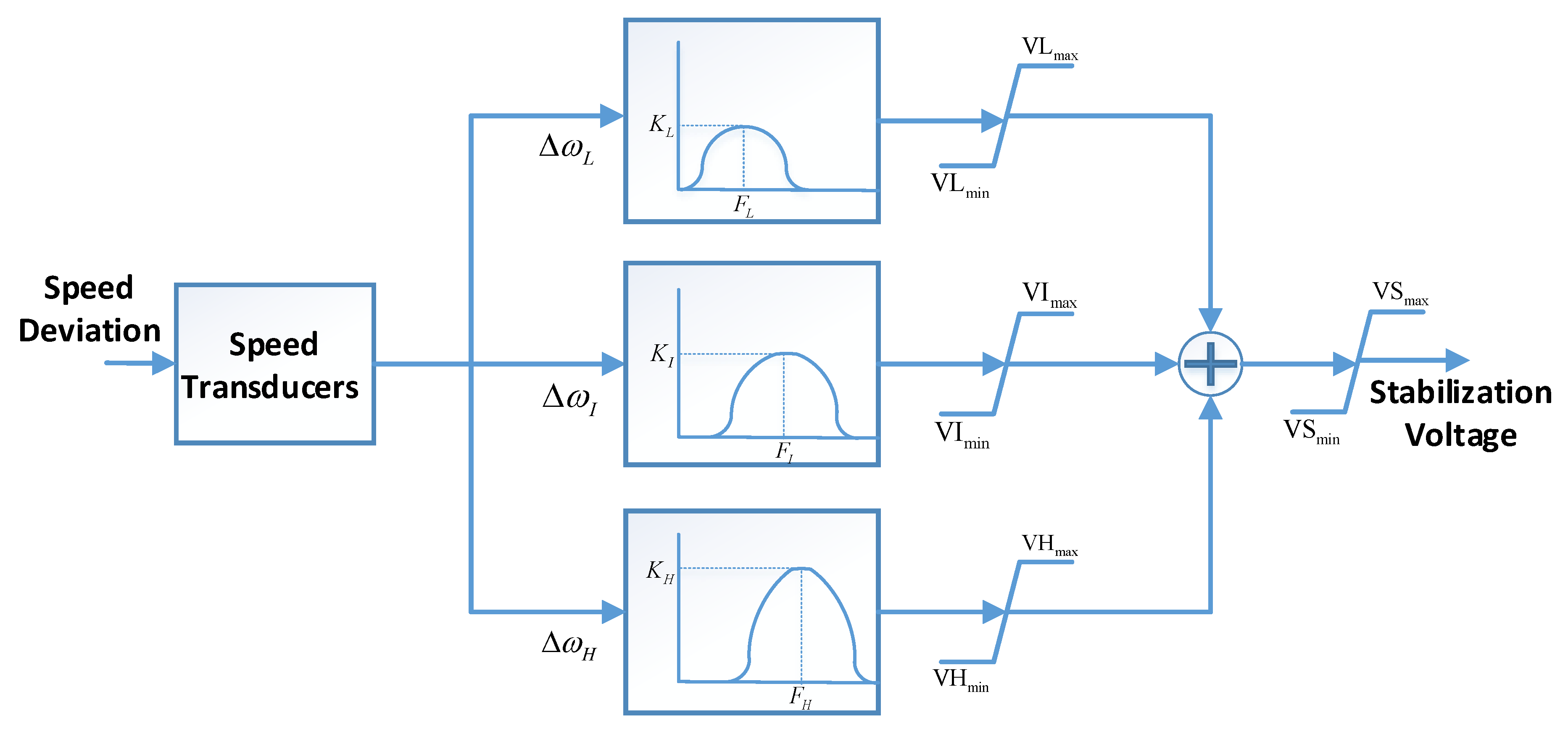
3.2.2. Multi-Band Power System Stabiliser

Multiband PSS (MBPSS) adjusts the working band to control different modes of oscillations. It separates the incoming speed deviation signal of the synchronous machine using three separate filters, high-pass, intermediate-pass, and low-pass filters, into high, intermediate, and low-frequency modes of oscillations, respectively [33]. The block diagram of MBPSS is shown in Figure 4. The MBPSS examines the stability in local-mode, inter-area-mode, and global-mode of oscillation. In the local-mode, the oscillations occur between a unit and the rest of the generating station, and it is dealt with using the high-pass filter. The inter-area-mode oscillations occur between two groups of generation plants, and they are dealt with using the intermediate-pass filter. The global-mode oscillations take place in all the generators in the isolated power system, and they are dealt with using the low-pass filter. This is in direct contrast to the GPSS, which focuses only on the local-mode instability of the system. Finally, the outputs of all three bands are summed and passed through an output limiter to produce the MBPSS output signal.

3.3. Flexible AC Transmission System

Flexible AC transmission system (FACTS) devices can furnish series or shunt compensation to the reactance of the lines to which they are connected. These devices also provide damping of oscillations in the power grid [34]. Thus, they can reduce the power delivery costs, improve grid stability, and enhance the controllability of the networks. In this work, the shunt compensation is studied through static var compensator and static synchronous compensator.

3.3.1. Static Var Compensator

The static var compensator (SVC) is a shunt-type device regulating the voltage and power flow and can enhance the transient stability on power grids. According to the system reference voltage, the SVC either injects or absorbs reactive power to regulate the voltage on the network. The SVC provides reactive power to the system and acts capacitive if the system voltage is lower than the reference voltage. On the contrary, the SVC absorbs reactive power from the system and acts inductive if the system voltage is higher than the reference voltage [35]. A simplified single-wire circuit diagram of an SVC using the thyristor controlled reactor and thyristor switched capacitor is illustrated in Figure 5. The SVC system comprises banks of three-phase capacitors and inductors that are linked to the secondary side of a coupling transformer. The regulating system of the SVC comprises a pulse generator, a synchronising unit, a voltage measurement unit, a voltage regulator, and a distribution unit.

3.3.2. Static Synchronous Compensator

The static synchronous compensator (STATCOM) is a voltage source converter (VSC)-based FACTS device. In addition to a VSC, it consists of a coupling transformer and a controller [35]. A simplified single-line diagram of a STATCOM is illustrated in Figure 6. The STATCOM autonomously regulates system voltage by either absorbing or generating reactive power. Opposite to the SVC, the STATCOM output current can be regulated independently from the AC system voltage. STATCOM has a dynamic response time of less than 10 ms compared to the SVC, which has a response of around 20 to 30 ms. Over other shunt-type compensators, the STATCOM has a possible active harmonic filter capability and offers equal lag and lead output. It also provides fast response and continuous reactive power control.

4. Connection, Interaction, and Coordination among Nuclear Power Plant, Grid, and Protection Systems

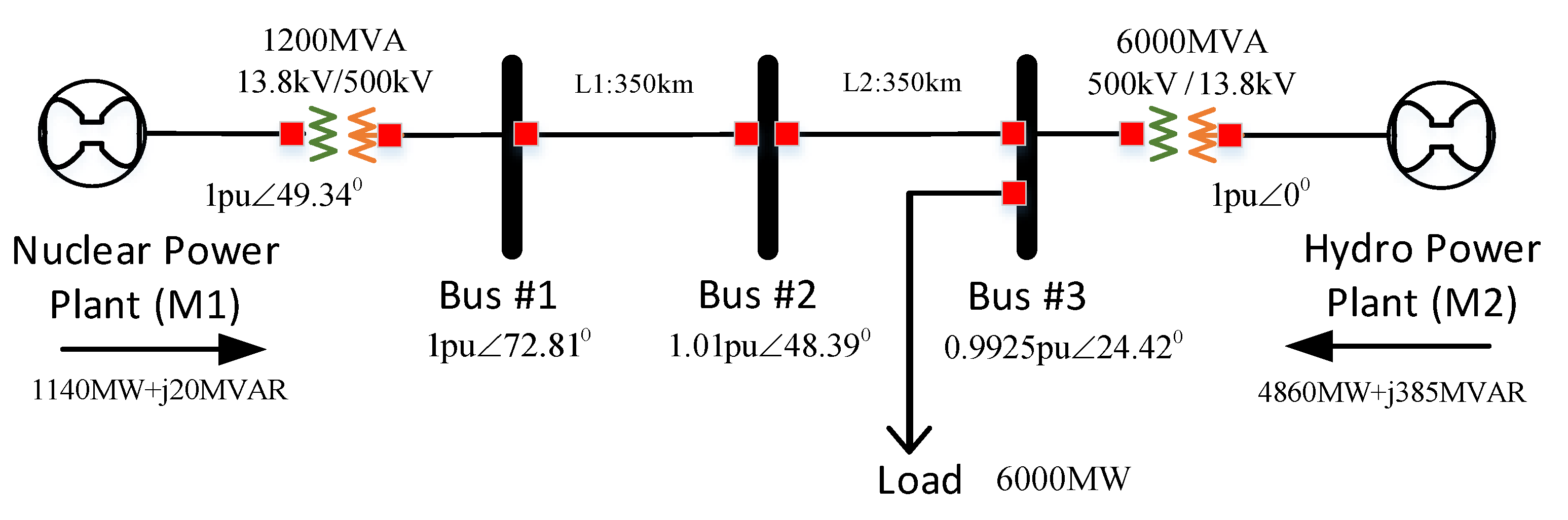
4.1. Connection

For reliable and secure operation of a nuclear power plant, the International Atomic Energy Agency (IAEA) guidelines suggest that at least two independent connections should be furnished between a nuclear power plant and the grid [36]. The first connection is to transfer the power from the nuclear plant generator to the grid via the generator transformer, whereas the second connection is to supply the nuclear plant via the station transformer in the absence of the first connection. The power output involves a double circuit overhead high-voltage line in addition to cable lines to reduce the risk of a breakdown in case of adverse weather. A nuclear power plant requires a highly stable and reliable grid supply for their auxiliaries and safety systems. The nuclear plant safety systems are provided from various sources such as generators, independent diesel generators, distribution grids, high voltage grids, and battery banks [37]. Usually, all the station auxiliaries are supplied via the unit transformers, or half of the auxiliaries is served from the unit transformers and the other half is served via the station transformer to avoid common cause failures. The generator transformers and station transformers can be connected to the same substation provided that there is sufficient separation between the two connections. Alternatively, they can be connected to separate substations operating at different voltages. For a reliable off-site supply, a sufficient number of transmission circuit connections from the substations to the rest of the transmission system are also required. Measures are also needed to ensure that the substations and transmission circuits are sufficiently robust to withstand extreme events and natural disasters.

4.2. Interaction

The performance of a nuclear power plant is influenced by the electric grid. A nuclear power plant needs to stay connected to the grid, even in the presence of disturbances. Severe frequency and voltage disturbances may gravely influence the availability, reliability, and operability of a nuclear plant in the short as well as in the long term [15]. A prolonged voltage reduction will result in amplification of the excitation current of the generator, which may lead to overheating and may potentially cause generator tripping. In the case of large load-loss in the grid, the grid voltage will change steeply and generators may become unstable or be tripped by V/Hz relays. Thus, generators are supplied with an over-excitation limiter and protection system to avoid these issues [11]. During oversupply of active power in the grid, the grid frequency may increase, and this will lead to an over-frequency condition, which will further affect the pressure and temperature variations in a nuclear power plant. The over-frequency relay, the turbine power control system, and the turbine-governor system act to keep the frequency at an acceptable level. The grid can sustain an off-nominal frequency for a considerable period; however, this may have mounting effects on the nuclear plant. For instance, this condition may cause damage to the turbine blades due to resonance. These variations also affect the auxiliary equipment of a nuclear power plant. Thus, during a disturbance, factors such as allowable operating-time and total-operating time play a significant role in warranting the secure and stable operation of a nuclear power plant [15,37].

4.3. Coordination

For the sake of a safe and stable operation, especially during frequency and voltage disturbances, strategies such as generation reduction, under-voltage load-shedding, and graded load-shedding must be carefully planned. Recent nuclear plant data show that a significant unscheduled downtime is due to disturbances in the power system [11]. Malfunctions in the power system produce variation in the grid frequency and voltage, which may upset the performance of the nuclear plant auxiliaries and may trigger relative relays. The nuclear plant protection system generally includes under- and over-frequency protection, V/Hz protection, under-voltage protection, a over-speed detection system, excitation system protection, reactor cooling cycle control, neutron flux control, thermal protection, and power swing-related protections. During events that cause a reduction in frequency, the under-frequency relays and load shed relays are one of the primary protectors for turbo-generators. The first trip of under-frequency relay results in a faster decline in system frequency. This may trigger the main pump under-speed relay and may trip the nuclear unit. During prolonged under-frequency conditions, the under-frequency relay may worsen active power shortage and triggers under-frequency load shed relays. The under-frequency protection system is employed to avert damage to the turbine. On the other hand, during events that cause the frequency to increase, the over-frequency relays, protect controllers, and generator trip relays should coordinate to control the over-frequency. Situations such as plant trip and cascaded load-shedding should be avoided. The coordination of excitation and protection systems also have a considerable effect on the dynamic voltage deviation as well as on the voltage stabilisation process. Over-excitation limiters, main pump relays, and under-voltage load shed relays are employed to maintain stable system voltage. Thus, steady and methodical coordination among nuclear plant, grid, auxiliary power subsystems, and protection systems is essential to implement operating strategies and emergency measures [11,37]. The alternating/direct current power supplies and distribution systems, instrumentation and control systems, and containment electrical penetration assemblies are class 1E electrical systems [38]. These systems are interfaced with the nuclear plant and with other systems.

Table A1. Protection system and their standards.

Protection System	Standard
AC distribution system, Electrical circuit	IEEE Std 242-1986
protection, Diesel generator protection
Motor protection system	IEEE Std 242-1986, IEEE Std C37.96-1988,
	IEEE Std 666-1991
Power transformer protection	IEEE Std C37.91-1985, IEEE Std 666-1991
Feeder circuit to power distribution	IEEE Std 141-1993, IEEE Std 242-1986
panel protection
Isolation and separation of non-class-1E	IEEE Std 384-1992
circuits from class-1E circuits
Surge protection of equipments and systems	IEEE Std 141-1993, IEEE Std 242-1986
Surge protection of induction motors	IEEE Std C37.96-1988
Protection of wire line facilities	IEEE Std 487-1992
Circuits with solid-state equipments	IEEE Std 518-1982
Surge arresters	IEEE Std C62.2-1987
Surge voltage determination	IEEE Std C62.41-1991
Surge withstand capability	IEEE Std C62.45-1992
Protection for batteries	IEEE Std 946-1992
Protection of battery chargers, inverters	IEEE Std 446-1987
Ground protection practices	IEEE Std 142-1991, IEEE Std C62.92.3-1993
Alarms and indication	IEEE Std 944-1986
Electrical penetration	IEEE Std 317-1983

in Appendix A mentions the standards employed by the protection system for these systems [39].

5. Simulation Cases, Results, and Discussion

Here, the behaviour of the nuclear power plant and different network variables is studied in the presence of single-phase and three-phase faults. The behaviour of the plant is also studied following a permanent load-loss event. Figure 7 shows the line diagram of an electric grid with two generators that have a total electrical power generation capacity of 7.2 GW. The nuclear power plant (M1) has a 1.2 GWe capacity, and the hydro power plant (M2) has a 6 GWe capacity. The values of the parameters of all components of the model are given in

Table A2. Parameter values of the components of the model.

Generator 1 and 2
Line-to-Line	Frequency	Stator	Inertia	Pole	Reactances
Voltage (kV)	(Hz)	Resistance (pu)	Coefficient (s)	Pairs	(pu)
13.8	60	0.002854	3.7	32	$Xd=1.305$, $X{d}^{{}^{\prime }}=0.296$, $X{d}^{{}^{″}}=0.252$,
					$Xq=0.474$, $X{q}^{{}^{″}}=0.243$, $Xl=0.180$
Excitation System 1 and 2
LPF Time	Regulator	Regulator Time	Damping	Damping Filter	Exciter	Exciter Time
Constant (s)	Gain	Constant (s)	Filter Gain	Time Constant (s)	Gain	Constant (s)
0.02	200	0.001	0.001	0.1	1	0
Generic PSS
Sensor Time	Gain	Wash-out Time	Lead-Lag 1 Time Constant (s)		Lead-Lag 2 Time Constant (s)
Constant (s)		Constant (s)
0.015	2	0.7	$T_{num}=0.06$, $T_{den}=0.5$		$T_{num}=0$, $T_{den}=0$
Multiband PSS
Global	Low	Low Frequency	Intermediate	Intermediate	High	High Frequency
Gain	Frequency (Hz)	Gain	Frequency (Hz)	Frequency Gain	Frequency (Hz)	Gain
1.0	0.025	5	0.8	25	12	145
SVC
Nominal	Frequency	Three-phase Base		Average Time	Droop	Voltage Regulator
Voltage (kV)	(Hz)	Power (MVA)		Delay (ms)	(pu/Pbase)	Gain (puB/puV/s)
500	60	200		4	0.03	300
STATCOM
Nominal	Frequency	Converter	Converter		DC Link	DC Link
Voltage (kV)	(Hz)	Rating (MVA)	Impedance (pu)		Voltage (kV)	Capacitance (F)
500	60	100	$R=0.0073$, $L=0.22$		40	350
Maximum Voltage	Droop	${\mathit{V}}_{\mathit{a}\mathit{c}}$Regulator	${\mathit{V}}_{\mathit{d}\mathit{c}}$Regulator		Current Regulator
Rate (pu/s)	(pu)	Gains	Gains		Gains
10	0.03	$K_p=5$, $K_i=1000$	$K_p=0.0001$, $K_i=0.02$		$K_p=0.3$, $K_i=10$, $K_f=0.22$

of Appendix A.

5.1. Case I: Response under Single-Phase Fault

A load-following operation of the nuclear plant is considered to analyse the system response in the presence of multiple single-phase faults. Here, three single-phase faults, each of 100 ms duration, is applied on bus 1 at 500 s, 900 s, and 1200 s. Initially, the nuclear power plant is run at 95% full power and the following power set-point sequence is considered:

$$\begin{array}{ccc}\hfill P_n^{ref}& =& \left\{\begin{array}{cc}0.95,\hfill & 0\le t\le 200\hfill \\ -0.0584(t-200)/60+0.95,\hfill & 200<t\le 700\hfill \\ 0.4633,\hfill & 700<t\le 1000\hfill \\ 0.0584(t-700)/60+0.4633,\hfill & 1000<t\le 1500\hfill \\ 0.95,\hfill & 1500<t\le 2000\hfill \end{array}\right.\hfill \end{array}$$

(47)

The impact of faults on system stability is observed with generic PSS and multi-band PSS connected to the AVRs of M1 and M2. It is observed that the system becomes unstable in the absence of PSS. In the presence of PSS, the system stability can be analysed by assessing different network variables as shown in Figure 8. The rotor angle difference between the two plants is shown in Figure 8a. The rotor speeds of both plants are shown in Figure 8b. It can be noticed that, during the presence of fault, the speed of M1 rises as its electrical power is lower than its mechanical power. It can also be observed that there are oscillations present at a low frequency after fault clearing. The GPSS is able to damp the 0.8 Hz oscillations; however, it is not effective at damping the 0.025 Hz mode. The MBPSS can efficiently damp both the 0.8 Hz and the 0.025 Hz oscillations. The MBPSS rejects the fault disturbance earlier than the GPSS and has a lower settling time. The variation in terminal voltage and the voltage positive sequence are shown in Figure 8c,d, respectively. The variation in the mechanical power output of the nuclear plant and the control signal to the turbine-governor valve are illustrated in Figure 8e,f, respectively. It is observed that the turbine power output can follow the reference variations. Figure 8g,h show the variation in core neutronic power and total reactivity, respectively. The variation in other nuclear plant variables are given in Figure 9, in which Figure 9a depicts the fuel temperature, Figure 9b shows the coolant temperature, Figure 9c shows the reactor plenum temperature, Figure 9d shows the steam generator plenum temperature, Figure 9e shows the hot and cold leg temperatures, Figure 9f shows the PCL temperatures, Figure 9g shows the MTL temperatures, and Figure 9h shows the pressuriser pressure. It has been observed that, in both cases, the system can handle multiple single-phase faults. The effect of faults on the plant side is suppressed by the PSS. The response of nuclear power plant variables shows that the GPSS gives oscillations after fault clearing. On the contrary, the MBPSS produces smooth variations in the plant signal and gives an oscillation-free response.

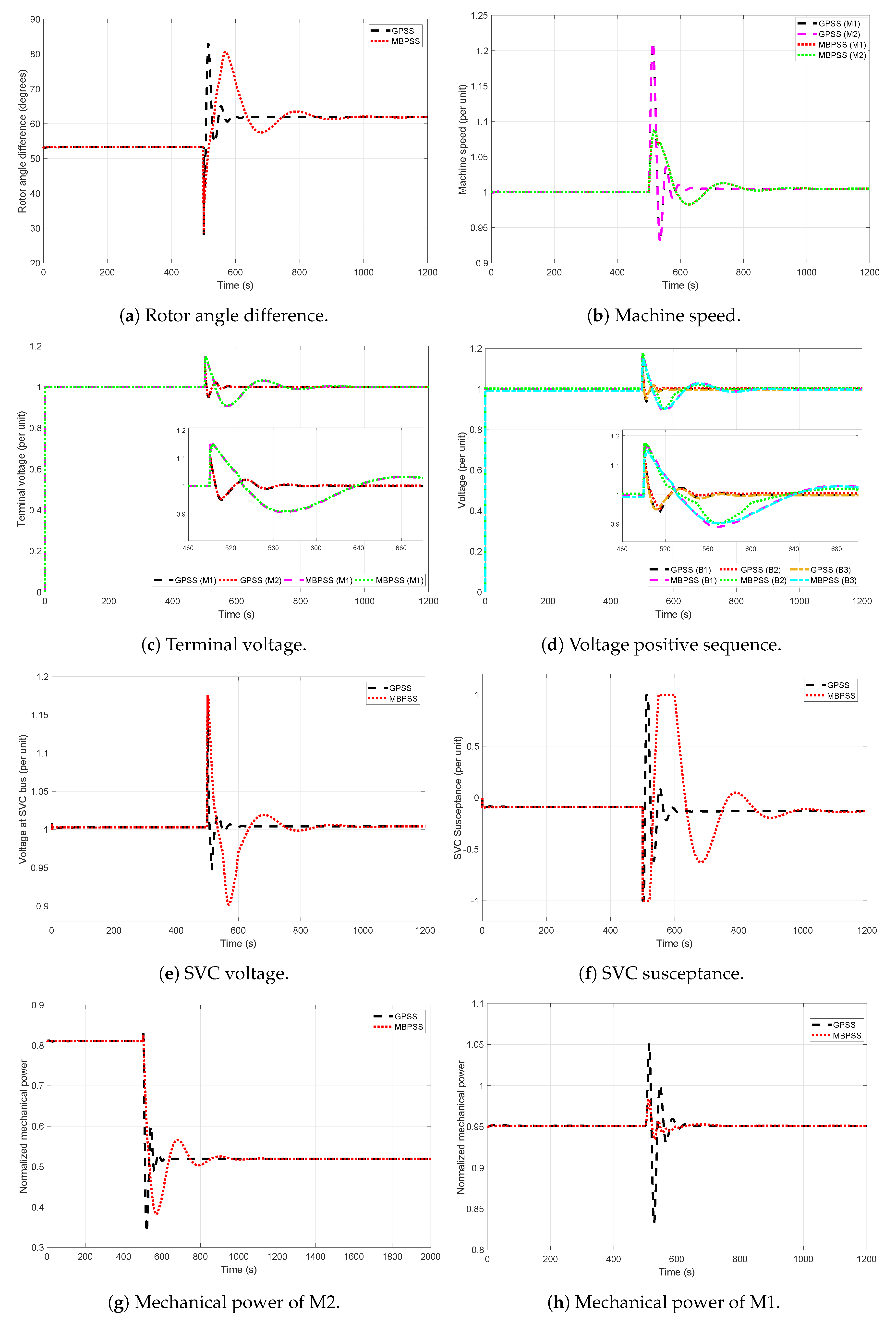
5.2. Case II: Response under Three-Phase Fault

In this section, the responses of the network and the plant variables are studied in the presence of three-phase faults. Here, four three-phase faults, each of 100 ms duration, are applied on bus 1 at 200 s, 500 s, 1000 s, and 1500 s. To study the response of the plant for a sudden variation in the load, a large ramp variation in the load is applied. This type of sudden load decrement transient reflects a restart after a shutdown scenario. The nuclear power plant is run at 95% full power, and the transient is given as follows:

$$\begin{array}{ccc}\hfill P_n^{ref}& =& \left\{\begin{array}{cc}0.95,\hfill & 0\le t\le 220\hfill \\ -1.608(t-220)/60+0.95,\hfill & 220<t\le 250\hfill \\ 0.146,\hfill & 250<t\le 800\hfill \\ 0.05856(t-800)/60+0.146,\hfill & 800<t\le 1200\hfill \\ 0.5364,\hfill & 1200<t\le 1400\hfill \\ 0.05856(t-1400)/60+0.5364,\hfill & 1400<t\le 1800\hfill \\ 0.95,\hfill & 1800<t\le 2000\hfill \end{array}\right.\hfill \end{array}$$

(48)

The impact of faults on system stability is first analysed for the case with a PSS at each generator but without FACTS compensation. It is observed from the rotor angle difference signal that the two machines quickly fall out of synchronism after fault clearing even in the presence of GPSS or MBPSS. The PSS alone is unable to keep the machines in sync. To mitigate this, a FACTS device is included in addition to the PSS at each generator to stabilise the network in the event of a three-phase fault contingency.

5.2.1. PSS and SVC

In this case, the transmission line is shunt compensated at bus 2 by an SVC. During the steady-state condition of the system, the reference voltage is manipulated per the load flow value of the bus voltage. Any variance in the voltage signal is compensated by the SVC. If the voltage is lower than the reference voltage, then the SVC injects reactive power on the line. However, the action of an SVC does not affect the damping torque of the system. Figure 10 shows the impact of three-phase faults on system stability having PSSs coupled with AVRs of M1 and M2 along with the SVC connected at bus 2. Figure 10a illustrates the variation in rotor angle difference, Figure 10b shows the machine speeds, Figure 10c shows the variation of terminal voltage, Figure 10d shows the voltage positive sequence, Figure 10e shows the SVC voltage, and Figure 10f shows the SVC susceptance. From the figures, it is observed that the case involving GPSS and an SVC produces large but damped oscillations with a frequency of 0.025 Hz. The speeds of the system generation units also swing together with the 0.025 Hz oscillation after fault clearing. The power system for the case of GPSS and SVC could not damp low-frequency oscillation, whereas the system with MBPSS and SVC is able to damp the oscillations and produces a smoother response of the variables. The variation in the mechanical power output of the turbine and the control signal to the valve are given in Figure 10g,h, respectively. The PI controller output can track the reference variation in both cases. The variation of other plant variables are illustrated in Figure 11, in which Figure 11a depicts the change in core neutronic power, Figure 11b depicts the change in total reactivity, Figure 11c shows the fuel temperature, Figure 11d shows the coolant temperature, Figure 11e shows the hot and cold leg temperatures, Figure 11f shows the PCL temperatures, Figure 11g shows the MTL temperatures, and Figure 11h shows the pressuriser pressure. It is observed from the results that the system involving SVC and PSS can handle multiple three-phase faults. However, the response of nuclear power plant variables in the cases of GPSS and SVC is unable to damp the oscillations after fault clearing, which may severely affect the performance of the plant during recurring fault conditions. On the contrary, the system involving MBPSS and SVC was able to damp the oscillations and produces smooth plant response. Thus, the combination of MBPSS and SVC is recommended to handle severe three-phase faults.

5.2.2. PSS and STATCOM

In this case, the STATCOM is employed to test the efficacy of the coupling using PSSs at M1 and M2 and a shunt compensated FACTS device at bus 2. The impact of three-phase faults on system stability is studied for case involving GPSS and STATCOM, and MBPSS and STATCOM, as demonstrated in Figure 12. Figure 12a depicts the variation in rotor angle difference, Figure 12b shows the machine speeds, Figure 12c shows the variation in terminal voltage, Figure 12d shows the voltage positive sequence, Figure 12e shows the STATCOM voltage, and Figure 12f shows the STATCOM susceptance. It can be noted that the case involving GPSS and STATCOM is unable to damp the 0.025 Hz oscillations after fault clearing. On the other hand, the MBPSS and STATCOM combination can damp the oscillations and produces a smooth response. The variation in mechanical power output of the nuclear power plant and the control signal to the valve are shown in Figure 12g,h, respectively. The output of the turbine PI controller is steadily able to follow the reference variation in both cases. The variation in other plant variables are shown in Figure 13, in which Figure 13a depicts the variation of core neutronic power, Figure 13b shows the variation in total reactivity, Figure 13c shows the fuel temperature, Figure 13d shows the coolant temperature, Figure 13e shows the hot and cold leg temperatures, Figure 13f shows the PCL temperatures, Figure 13g shows the MTL temperatures, and Figure 13h shows the pressuriser pressure. The response of various nuclear power plant variables when GPSS and STATCOM operate cannot fully damp the oscillations after fault clearing. Contrarily, the MBPSS and STATCOM system can damp the oscillations and produces smooth plant response. It can be noted from the figures that the system with STATCOM and PSS can handle multiple three-phase faults better than the SVC with the PSS system. The STATCOM-based system can also damp the oscillations better than that of the SVC-based system. In case of a STATCOM, the maximum capacitive power reduces linearly with voltage decrease due to a constant current, whereas in the case of an SVC, it is proportional to the square of the system voltage due to constant susceptance. Thus, the STATCOM can provide more capacitive power during a fault as compared to the SVC.

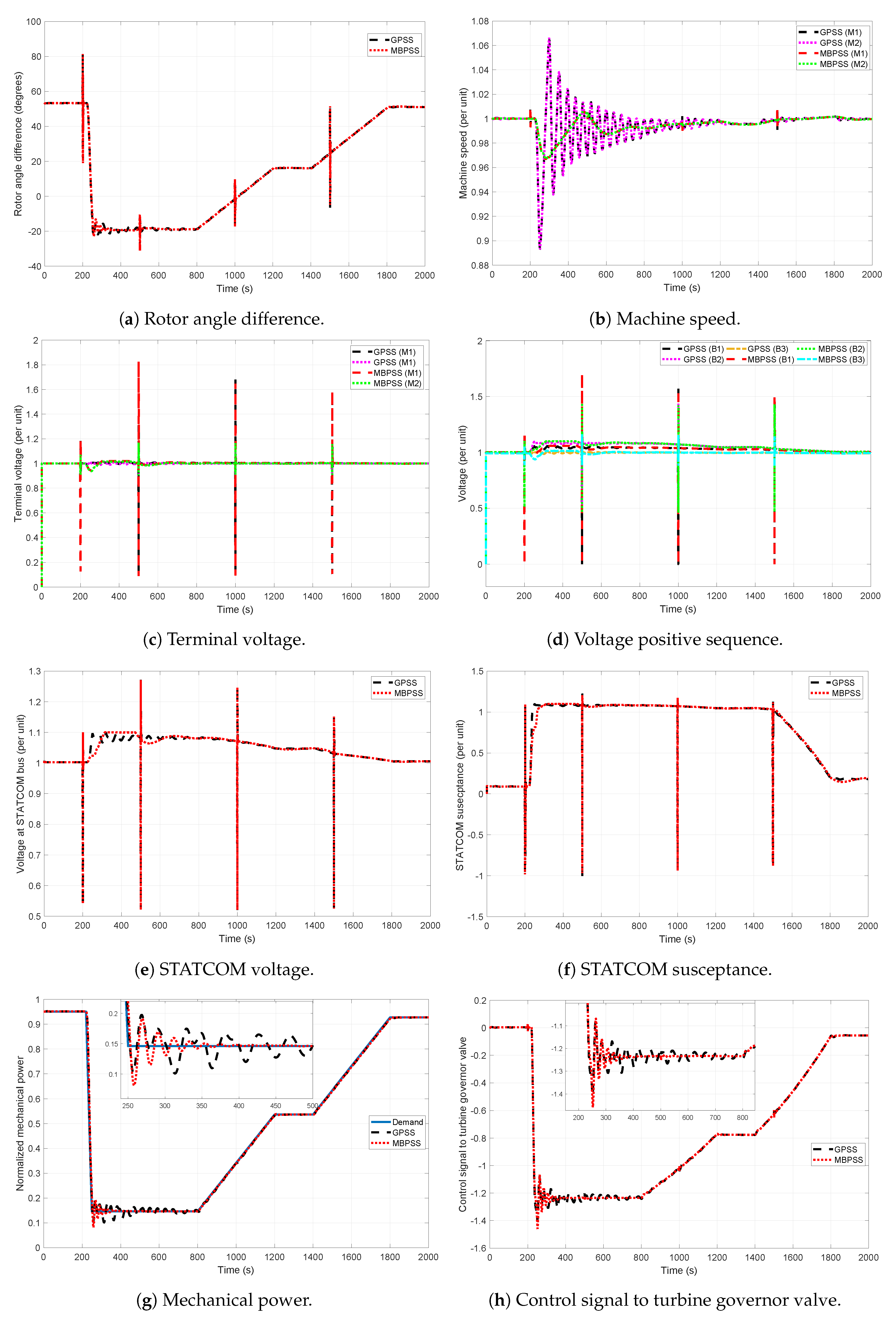
5.3. Case III: Response under Permanent Load Loss

In this section, the responses of the network and the plant variables are studied during a permanent load-loss from the electric grid. Initially, the hydro power plant (M2) was run at 81% full-power. At $t=500$ s, a permanent load-loss at bus 3 of 1800 MW was considered, which caused the hydro-power plant to decrease the power output to a steady-state value of 51%. The impact of the permanent load-loss on system stability was studied in the case with PSSs at M1 and M2 and a shunt FACTS device connected to bus 2. Similar to the three-phase fault case, the two machines fall out of synchronism if no shunt FACTS device is present. Thus, a shunt FACTS device was incorporated at bus 2 to keep the network stable during the load-loss transient. Here, an SVC and a STATCOM were considered as alternatives to stabilise the network during a permanent load-loss situation, together with PSS at M1 and M2.

5.3.1. PSS and SVC

The system stability was studied following a permanent load-loss event for the case with GPSS and MBPSS along with an SVC in operation, as demonstrated in Figure 14. Figure 14a shows the variation in rotor angle difference, Figure 14b shows the machine speeds, Figure 14c shows the variation in terminal voltage, Figure 14d shows the voltage positive sequence, Figure 14e shows the SVC voltage, and Figure 14f shows the SVC susceptance. The variation in mechanical power output of the HPP is shown in Figure 14g. The permanent load-loss transient at the electric grid reduces the power output at the HPP. The turbine speed controller at the HPP can handle the large permanent load-loss transient. The PI controller during the GPSS produces a 35.19% peak undershoot in the mechanical power output of the HPP, whereas the MBPSS produces a 26.54% peak undershoot. The variation in the mechanical power output of the turbine is shown in Figure 14h. The turbine speed controller at the nuclear plant can maintain a steady-state in both cases. Use of the GPSS results in a transient with $\pm 11.48$ variation in the mechanical power output of the nuclear plant, whereas the MBPSS results in a power variation within $\pm 2.54$. Moreover, the MBPSS can damp the oscillations better than the GPSS. The variation in other plant variables are shown in Figure 15, in which Figure 15a depicts the change in core neutronic power, Figure 15b depicts the change in the control signal to the valve, Figure 15c shows the total reactivity, Figure 15d shows the fuel temperature, Figure 15e shows the coolant temperature, Figure 15f shows the hot and cold leg temperatures, Figure 15g shows the PCL temperatures, and Figure 15h shows the MTL temperatures. From the figures, it can be observed that both the MBPSS with SVC and the GPSS with SVC can handle the permanent load loss situation at the nuclear power plant, in which the MBPSS-based system produces fewer variations in the nuclear power plant variables compared to the GPSS-based system.

5.3.2. PSS and STATCOM

In this case, the system stability following a permanent load-loss at bus 3 is studied for the case with PSS and STATCOM in operation, as demonstrated in Figure 16. Figure 16a depicts the change in rotor angle difference, Figure 16b shows the machine speeds, Figure 16c shows the variation of terminal voltage, Figure 16d shows the voltage positive sequence, Figure 16e shows the STATCOM voltage, and Figure 16f shows the STATCOM susceptance. The variation in the mechanical power output of the HPP is shown in Figure 16g. The turbine speed controller at the HPP can handle the large permanent load-loss transient. The PI controller during the GPSS produces a 36.73% peak undershoot in the mechanical power of HPP, whereas the MBPSS produces a 26.21% peak undershoot. The variation in the mechanical power output of the nuclear plant is shown in Figure 16h. The turbine speed controller at the nuclear plant can maintain a steady state in both cases. Use of the GPSS results in a transient with $\pm 11.43$ variation in the mechanical power output of the nuclear plant, whereas use of the MBPSS results in a mechanical power variation within $\pm 2.47$. In addition, the MBPSS can damp the oscillations better than the GPSS. The variation in other nuclear plant variables are shown in Figure 17, in which Figure 17a shows the variation in core neutronic power, Figure 17b depicts the change in the control signal to the valve, Figure 17c shows the total reactivity, Figure 17d shows the fuel temperature, Figure 17e shows the coolant temperature, Figure 17f shows the hot and cold leg temperatures, Figure 17g shows the PCL temperatures, and Figure 17h shows the MTL temperatures. From the figures, it can be noted that the MBPSS and STATCOM produce fewer variations in the nuclear power plant variables compared to the GPSS and STATCOM. The STATCOM-based system works better than the SVC-based system as the STATCOM can impart more reactive power during a fault compared to the SVC and exhibits a swift response than the SVC.

6. Conclusions

The transient analysis of a simulated pressurised water-type nuclear power plant connected to a faulted electric grid was presented in this work. The plant model consists of various integrated subsystems, such as the core, thermal hydraulics, piping and plenum, pressuriser, steam generator, turbine, governor, dynamics shaft, actuator, sensor, and turbine-speed controller. The interactions between the nuclear power plant, the electric grid, and protection systems were studied under various scenarios including multiple single-phase faults, multiple three-phase faults, and the permanent load-loss events affecting the electricity grid. The dynamic performance of the nonlinear plant and that of the grid were analysed in the presence of transient stability enhancement components such as power system stabilisers, static var compensators, and static synchronous compensators. Furthermore, the load-following operation of the power plant was studied. The effectiveness of different compensation mechanisms was demonstrated on the interconnected nuclear plant/grid model using various simulations in the MATLAB/Simulink/Simscape environment. In this regard, the presented work moves forward research on the safety, reliability, and operability aspects of nuclear power and thus forms a platform for future research on the analysis of transient effects of power grid faults and disturbances in a nuclear power plant and on the devices that can be employed to mitigate such effects.

References

1. Maldonado, G.I. The performance of North American nuclear power plants during the electric power blackout of 14 August 2003. In Proceedings of the IEEE Symposium Conference Record Nuclear Science 2004, Rome, Italy, 16–22 October 2004; Volume 7, pp. 4603–4606. [Google Scholar]
2. Xuehao, H.; Xuecheng, Z.; Xiuming, Z.; Fulin, G.; Wenhua, Z. Pressurized water reactor nuclear power plant (NPP) modelling and the midterm dynamic simulation after NPP has been introduced into power system. In Proceedings of the TENCON ’93, IEEE Region 10 International Conference on Computers, Communications and Automation, Beijing, China, 19–21 October 1993; Volume 5, pp. 367–370. [Google Scholar]
3. Inoue, T.; Ichikawa, T.; Kundur, P.; Hirsch, P. Nuclear plant models for medium- to long-term power system stability studies. IEEE Trans. Power Syst. 1995, 10, 141–148. [Google Scholar] [CrossRef]
4. Ichikawa, T. Power Plant Dynamics Simulations Considering Interaction with Power System. In Proceedings of the IFAC Symposium on Control of Power Plants and Power Systems (CPSPP’97), Beijing, China, 18–21 August 1997; Volume 30, pp. 595–600. [Google Scholar]
5. Gao, H.; Wang, C.; Pan, W. A Detailed Nuclear Power Plant Model for Power System Analysis Based on PSS/E. In Proceedings of the 2006 IEEE PES Power Systems Conference and Exposition, Atlanta, GA, USA, 29 October–1 November 2006; pp. 1582–1586. [Google Scholar]
6. Li, X.; Liu, D.; Shi, X.; Zhao, J.; Wu, P. Research and Analyse for Pressurized Water Reactor Plant into Power System Dynamics Simulation. In Proceedings of the 2009 Asia-Pacific Power and Energy Engineering Conference, Wuhan, China, 28–30 March 2009; pp. 1–5. [Google Scholar]
7. Li, X.; Liu, D.; Wang, B.; Wu, P.; Zhao, J.; Shi, X. Dynamic characteristics analyse of pressurized water reactor Nuclear Power plant based on PSASP. In Proceedings of the 2009 4th IEEE Conference on Industrial Electronics and Applications, Xi’an, China, 25–27 May 2009; pp. 3629–3634. [Google Scholar]
8. Shi, X.; Wu, P.; Liu, D.; Li, X.; Zhao, J.; Zhang, Y.; Zhao, Z. Modeling and Dynamic Analysis of Nuclear Power Plant Reactor Based on PSASP. In Proceedings of the 2009 Asia-Pacific Power and Energy Engineering Conference, Wuhan, China, 28–30 March 2009; pp. 1–5. [Google Scholar]
9. Zhao, J.; Wu, P.; Liu, D. User-Defined Modeling of Pressurized Water Reactor Nuclear Power Plant Based on PSASP and Analysis of its Characteristics. In Proceedings of the 2009 Asia-Pacific Power and Energy Engineering Conference, Wuhan, China, 28–30 March 2009; pp. 1–6. [Google Scholar]
10. Othman, S.; Mahmoud, H.M.; Kotb, S.A. Interaction of a Nuclear Power Plant With the Egyptian Electrical Grid Based on PSS/E. In Proceedings of the 18th International Conference on Nuclear Engineering, Xi’an, China, 17–21 May 2010; Volume 1, pp. 27–32. [Google Scholar]
11. Wu, G.; Song, X.; Lin, J.; Zhong, W.; Liu, T.; Ye, X.; Ju, P. Coordinated protection and control between large capacity nuclear power plants and power grids. In Proceedings of the 2013 IEEE Power Energy Society General Meeting, Vancouver, BC, Canada, 21–25 July 2013; pp. 1–5. [Google Scholar]
12. Ju, P.; Wu, F.; Chen, Q.; Han, J.; Dai, R.; Wu, G.; Tang, Y. Model Simplification of Nuclear Power Plant for Power System Dynamic Simulation. In Proceedings of the 2018 International Conference on Control, Artificial Intelligence, Robotics Optimization (ICCAIRO), Prague, Czech Republic, 19–21 May 2018; pp. 260–266. [Google Scholar]
13. Wen, L.; Sheng, W.; Xu, Z. Comparative analysis of external characteristics of nuclear power units and thermal power units. In Proceedings of the 2019 IEEE Innovative Smart Grid Technologies—Asia (ISGT Asia), Chengdu, China, 21–24 May 2019; pp. 1051–1056. [Google Scholar]
14. Wang, L.; Zhao, J.; Liu, D.; Lin, Y.; Zhao, Y.; Lin, Z.; Zhao, T.; Lei, Y. Parameter Identification with the Random Perturbation Particle Swarm Optimization Method and Sensitivity Analysis of an Advanced Pressurized Water Reactor Nuclear Power Plant Model for Power Systems. Energies 2017, 10, 173. [Google Scholar] [CrossRef] [Green Version]
15. Wu, G.; Ju, P.; Song, X.; Xie, C.; Zhong, W. Interaction and Coordination among Nuclear Power Plants, Power Grids and Their Protection Systems. Energies 2016, 9, 306. [Google Scholar] [CrossRef] [Green Version]
16. Wang, L.; Sun, W.; Zhao, J.; Liu, D. A Speed-Governing System Model with Over-Frequency Protection for Nuclear Power Generating Units. Energies 2020, 13, 173. [Google Scholar] [CrossRef] [Green Version]
17. Poudel, B.; Joshi, K.; Gokaraju, R. A Dynamic Model of Small Modular Reactor Based Nuclear Plant for Power System Studies. IEEE Trans. Energy Convers. 2020, 35, 977–985. [Google Scholar] [CrossRef]
18. International Atomic Energy Agency. Introducing Nuclear Power Plants into Electrical Power Systems of Limited Capacity: Problems and Remedial Measures; International Atomic Energy Agency: Vienna, Austria, 1987. [Google Scholar]
19. Kirby, B.; Kueck, J.; Leake, H.; Muhlheim, M. Nuclear Generating Stations and Transmission Grid Reliability. In Proceedings of the 2007 39th North American Power Symposium, Las Cruces, New Mexico, 30 September–2 October 2007; pp. 279–287. [Google Scholar]
20. Wei-Jie, Z. Modeling and fault stability study for Million Kilowatts Nuclear Power Generator excitation system. In Proceedings of the 2014 International Conference on Power System Technology, Chengdu, China, 20–22 October 2014; pp. 244–250. [Google Scholar]
21. Shafei, M.A.R.; Ibrahim, D.K.; El-Zahab, E.E.A. Transient stability enhancement of Egyptian national grid including nuclear power plant in Dabaa area. In Proceedings of the 2012 IEEE International Conference on Power and Energy (PECon), Kota Kinabalu, Malaysia, 2–5 December 2012; pp. 487–492. [Google Scholar]
22. Abou-El-Soud, A.; Elbanna, S.H.A.; SABRY, W. A Strong Action Power System Stabilizer Application in a Multi-machine Power System Containing a Nuclear Power Plant. In Proceedings of the 2019 16th Conference on Electrical Machines, Drives and Power Systems (ELMA), Varna, Bulgaria, 6–8 June 2019; pp. 1–6. [Google Scholar]
23. Kerlin, T.W. Dynamic Analysis and Control of Pressurized Water Reactors; Academic Press: Cambrige, MA, USA, 1978; Volume 14, pp. 103–212. [Google Scholar]
24. Ali, M.R.A. Lumped Parameter, State Variable Dynamic Models for U-Tube Recirculation Type Nuclear Steam Generators. Ph.D. Dissertation, University of Tennessee, Knoxville, TN, USA, 1976. [Google Scholar]
25. Naghedolfeizi, M. Dynamic Modeling of a Pressurized Water Reactor Plant for Diagnostics and Control. Master’s Thesis, University of Tennessee, Knoxville, TN, USA, 1990. [Google Scholar]
26. Vajpayee, V.; Becerra, V.; Bausch, N.; Deng, J.; Shimjith, S.R.; Arul, A.J. Dynamic Modelling, Simulation, and Control Design of a Pressurized Water-type Nuclear Power Plant. Nucl. Eng. Des. 2020, 370, 110901. [Google Scholar] [CrossRef]
27. Milano, F. Power System Modelling and Scripting. In Power Systems; Springer: Berlin/Heidelberg, Germany, 2010. [Google Scholar]
28. Vajpayee, V.; Becerra, V.; Bausch, N.; Deng, J.; Shimjith, S.; Arul, A.J. Robust-optimal integrated control design technique for a pressurized water-type nuclear power plant. Prog. Nucl. Energy 2021, 131, 103575. [Google Scholar] [CrossRef]
29. Vajpayee, V.; Becerra, V.; Bausch, N.; Deng, J.; Shimjith, S.; Arul, A.J. LQGI/LTR based robust control technique for a pressurized water nuclear power plant. Ann. Nucl. Energy 2021, 154, 108105. [Google Scholar] [CrossRef]
30. Subudhi, C.S.; Bhatt, T.U.; Tiwari, A.P. A Mathematical Model for Total Power Control Loop of Large PHWRs. IEEE Trans. Nucl. Sci. 2016, 63, 1901–1911. [Google Scholar] [CrossRef]
31. Kundur, P.; Paserba, J.; Ajjarapu, V.; Andersson, G.; Bose, A.; Canizares, C.; Hatziargyriou, N.; Hill, D.; Stankovic, A.; Taylor, C.; et al. Definition and classification of power system stability IEEE/CIGRE joint task force on stability terms and definitions. IEEE Trans. Power Syst. 2004, 19, 1387–1401. [Google Scholar] [CrossRef]
32. Kundur, P. Power System Stability and Control; EPRI Power System Engineering Series McGraw-Hill: New York, NY, USA, 1994. [Google Scholar]
33. Grondin, R.; Kamwa, I.; Soulieres, L.; Potvin, J.; Champagne, R. An approach to PSS design for transient stability improvement through supplementary damping of the common low-frequency. IEEE Trans. Power Syst. 1993, 8, 954–963. [Google Scholar] [CrossRef]
34. Zhang, X.P.; Rehtanz, C.; Pal, B. FACTS-Devices and Applications; Flexible AC Transmission Systems: Modelling and Control; Springer: Berlin/Heidelberg, Germany, 2012; pp. 1–30. [Google Scholar]
35. Hingorani, N.G.; Gyugyi, L. Understanding FACTS: Concepts and Technology of Flexible AC Transmission Systems; Wiley-IEEE Press: Piscataway, NJ, USA, 2000. [Google Scholar]
36. International Atomic Energy Agency. Electric Grid Reliability and Interface with Nuclear Power Plants; Number NG-T-3.8 in Nuclear Energy Series; International Atomic Energy Agency: Vienna, Austria, 2012. [Google Scholar]
37. Łowczowski, K. Nuclear Power Plants in the National Power System. Acta Energet. 2018, 2, 70–75. [Google Scholar]
38. Mazzoni, O.S. Electrical Systems for Nuclear Power Plants; IEEE Press Wiley: Piscataway, NJ, USA, 2019. [Google Scholar]
39. IEEE. IEEE Standard for Criteria for the Protection of Class 1E Power Systems and Equipment in Nuclear Power Generating Stations; IEEE Std 741-2017 (Revision of IEEE Std 741-2007); IEEE Press Wiley: Piscataway, NJ, USA, 2017; pp. 1–63. [Google Scholar]
Figure 1. Block diagram representation of a pressurised water reactor (PWR)-type nuclear power plant connected to an electric grid.
Energies 14 01573 g001
Figure 2. Block diagram of turbine-speed control loop.
Energies 14 01573 g002
Figure 3. Block diagram representation of the generic power system stabiliser (PSS).
Energies 14 01573 g003
Figure 4. Block diagram representation of the multi-band PSS.
Energies 14 01573 g004
Figure 5. Block diagram representation of the static var compensator.
Energies 14 01573 g005
Figure 6. Block diagram representation of the static synchronous compensator.
Energies 14 01573 g006
Figure 7. Network model of an electric grid.
Energies 14 01573 g007
Figure 8. Case I: Variation in network signals during single-phase faults with generic and multiband PSS.
Energies 14 01573 g008
Figure 9. Case I: Variation in nuclear power plant variables following single-phase faults with generic and multiband PSS.
Energies 14 01573 g009
Figure 10. Case II.1: Variation in network signals during three-phase faults with generic and multiband PSS with a static var compensator (SVC).
Energies 14 01573 g010
Figure 11. Case II.1: Variation in nuclear power plant variables following three-phase faults with generic and multiband PSS with SVC.
Energies 14 01573 g011
Figure 12. Case II.2: Variation of network signals during three-phase faults with generic and multiband PSS with static synchronous compensator (STATCOM).
Energies 14 01573 g012
Figure 13. Case II.2: Variation of nuclear power plant variables during three-phase faults with generic and multiband PSS with STATCOM.
Energies 14 01573 g013
Figure 14. Case III.1: Variation in network signals during permanent load loss with generic and multiband PSS with SVC.
Energies 14 01573 g014
Figure 15. Case III.1: Variation in nuclear power plant variables during permanent load loss with generic and multiband PSS with SVC.
Energies 14 01573 g015
Figure 16. Case III.2: Variation in network signals during permanent load loss with generic and multiband PSS with STATCOM.
Energies 14 01573 g016
Figure 17. Case III.2: Variation in nuclear power plant variables during permanent load loss with generic and multiband PSS with STATCOM.
Energies 14 01573 g017
Publisher’s Note: MDPI stays neutral with regard to jurisdictional claims in published maps and institutional affiliations.