Research on the Fault Feature Extraction of Rolling Bearings Based on SGMD-CS and the AdaBoost Framework

Abstract

Symplectic geometric mode decomposition (SGMD) is a newly proposed signal processing method. Because of its superiority, it has gained more and more attention in the field of fault diagnosis. However, the similar component reorganization problem involved in this method has not been clearly stated. Aiming at this problem, this paper proposes the SGMD-CS method based on the SGMD method and the cosine similarity (CS) and has been compared and verified on the simulation signal and the actual rolling bearing signal. In addition, in order to realize the intelligent diagnosis of the wind turbine bearing fault, the symplectic geometric entropy (SymEn) is extracted as the fault feature and input it into the AdaBoost classification model. In summary, this paper proposes a new wind turbine fault feature extraction method based on the SGMD-CS and AdaBoost framework, and the validity of the method is verified by the rolling bearing vibration data of the Electrical Engineering Laboratory of Case Western Reserve University.

1. Introduction

As a clean energy source, wind power has developed rapidly in recent years because of its many advantages such as renewable energy and low pollution. With the continuous increase in the capacity of wind turbine machines around the world, the structure of these units has become increasingly complicated and coupled with their long-term use under harsh conditions, this places higher requirements on the fault diagnosis of wind turbines. Especially wind turbine bearings, as a key component for converting wind energy into electrical energy, have high failure rates and maintenance costs. In order to increase the output of wind turbines and reduce operation and maintenance costs, bearing status monitoring and fault diagnosis are essential to ensure the reliable and stable operation of wind turbines [1]. Because the fault will produce vibration, the vibration signal is collected by using the vibration sensor and analyzed to extract the hidden fault information to provide a basis for identifying the type of bearing fault. Regarding the placement of the sensors, literature [2] and [3] gave a new method to diagnose the damage of the transmission system bearings, that is, to measure vibration at the tower instead of the gearbox, which makes the measurement easier. And through the discussion of actual cases to study the reliability and effectiveness of this method for bearing fault detection.

No matter where the sensors are arranged, due to the randomness of wind energy, the load and speed of the bearing of the wind turbine will change accordingly, so the collected fault signals have the characteristics of nonlinear and nonstationary. The sampled vibration signal can be regarded as a time series, and a time series usually consists of different patterns. By decomposing it into a series of simple component sequences, judging and reconstructing these simple components, a large amount of information about the original state can be obtained. To obtain simple component sequences and reduce complexity, an effective signal decomposition method is needed that can separate components from the original signal effectively.

In the early days, the commonly used signal processing methods were fast Fourier transform and wavelet transform. The latter is based on wavelet basis functions, which can be regarded as adding a scale factor to the window function of the short-time Fourier transform (STFT), which makes up for the shortcomings of STFT. Therefore, it has been widely used in processing non-stationary signals. With the development of wavelet, wavelet packet, second-generation wavelet, multiwavelet, empirical mode wavelet, and flexible wavelet are proposed and applied one after another. Literature [4] compared the fast Fourier transform and wavelet transform comprehensively when monitoring the wind turbine bearing, reflecting the advantages of wavelet transform.

Since the choice of wavelet basis function in wavelet transform is based on experience and does not have adaptability, it has an important influence on the signal analysis results. Empirical mode decomposition (EMD), a new type of adaptive signal time-frequency processing method proposed by N.E. Huang and others in 1998 was based on the timescale characteristics of the data itself to decompose the complex signal into a finite number of intrinsic mode functions (IMF) [5]. Once this method was proposed, it has been widely used, but modal aliasing and end effects have appeared in the process of application. Therefore, many relevant scholars have done a lot of research here [6,7,8]. In addition, the local mean decomposition (LMD) proposed based on EMD has also been applied. It compensates for the shortcomings of the EMD method to a certain extent, mainly by adaptively decomposing the multi-component signal into several product functions (PF) [9]. This method is also widely used as an adaptive decomposition method [10].

The symplectic geometric spectrum method is a relatively new method of time series decomposition based on symplectic space compared to the traditional time series method based on Euclidean space. In symplectic geometry, since the symplectic matrix similar transformation is a normal transformation, it will not destroy the characteristics of the original time series, so when dealing with nonlinear problems, it has a better processing effect than singular spectral decomposition [11,12]. Regarding this method, relevant scholars have done a lot of research. Literature [13] estimated the embedding dimension of the symplectic geometric spectrum method and discussed the robustness of the method to noise, sequence length, and sampling interval in the study of time series. Literature [14] combined the symplectic geometry method and the principal component analysis method to study a chaotic time series. Literature [15] introduced the symplectic geometric spectral regression technique for the prediction of a nonlinear time series. The literature [16] and [17] decomposed the time series into the sum of some independent components based on symplectic geometry theory and derived a framework of this method. The literature [18] and [19] introduced the symplectic geometry algorithm to fault diagnosis and obtained good results. In addition, the method was introduced to modal parameter identification [20], vibration feature parameter identification for structural health monitoring [21], and the analysis of athlete’s surface EMG signals [22].

In the process of decomposing the original time series using the symplectic geometry method, the initially obtained components are not completely independent, so components with the same characteristics need to be reorganized. Regarding how to reorganize, most of the literature does not give a detailed description. Literature [23] used an iterative approach, starting with the first component and looking for similar components with it. When the normalized mean square error (NMSE) of the residual signal and the original signal is less than the given threshold, the iteration stops, and the final recombination components are determined. However, there is still no clear description on how to determine similar components. In this paper, the cosine similarity (CS) is introduced to measure the similarity between components for the problem of component reorganization. As a method of measuring similarity, cosine similarity is widely used in file comparison and text mining but rarely used in signal processing [24,25]. This paper introduces cosine similarity for the first time in the decomposition process of the symplectic geometric spectrum and constructs a cosine similarity matrix to seek components with the same characteristics and reorganize them.

The traditional fault diagnosis method based on the aforementioned signal processing technology has some shortcomings, and with the development of artificial intelligence technology, this brings new ideas to fault identification [26]. In this paper, based on the SGMD-CS method and machine learning theory, through calculating the symplectic geometric entropy as a feature vector and transporting it to the constructed AdaBoost classifier, so as to obtain intelligent fault diagnosis [27]. The main contributions and novelty of this paper are as follows:

(1)

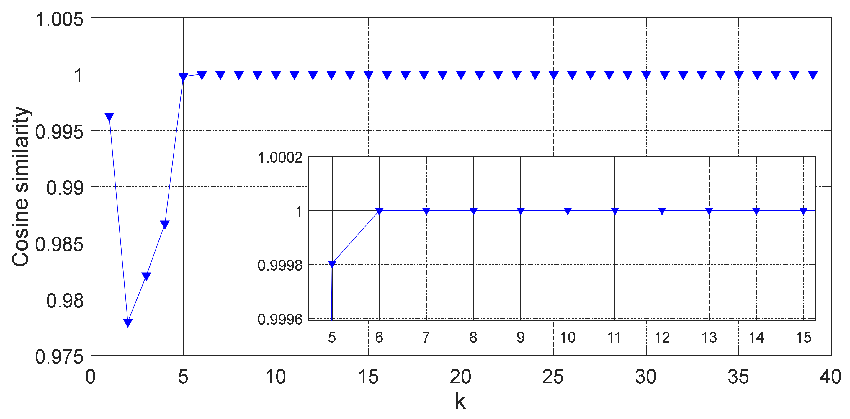
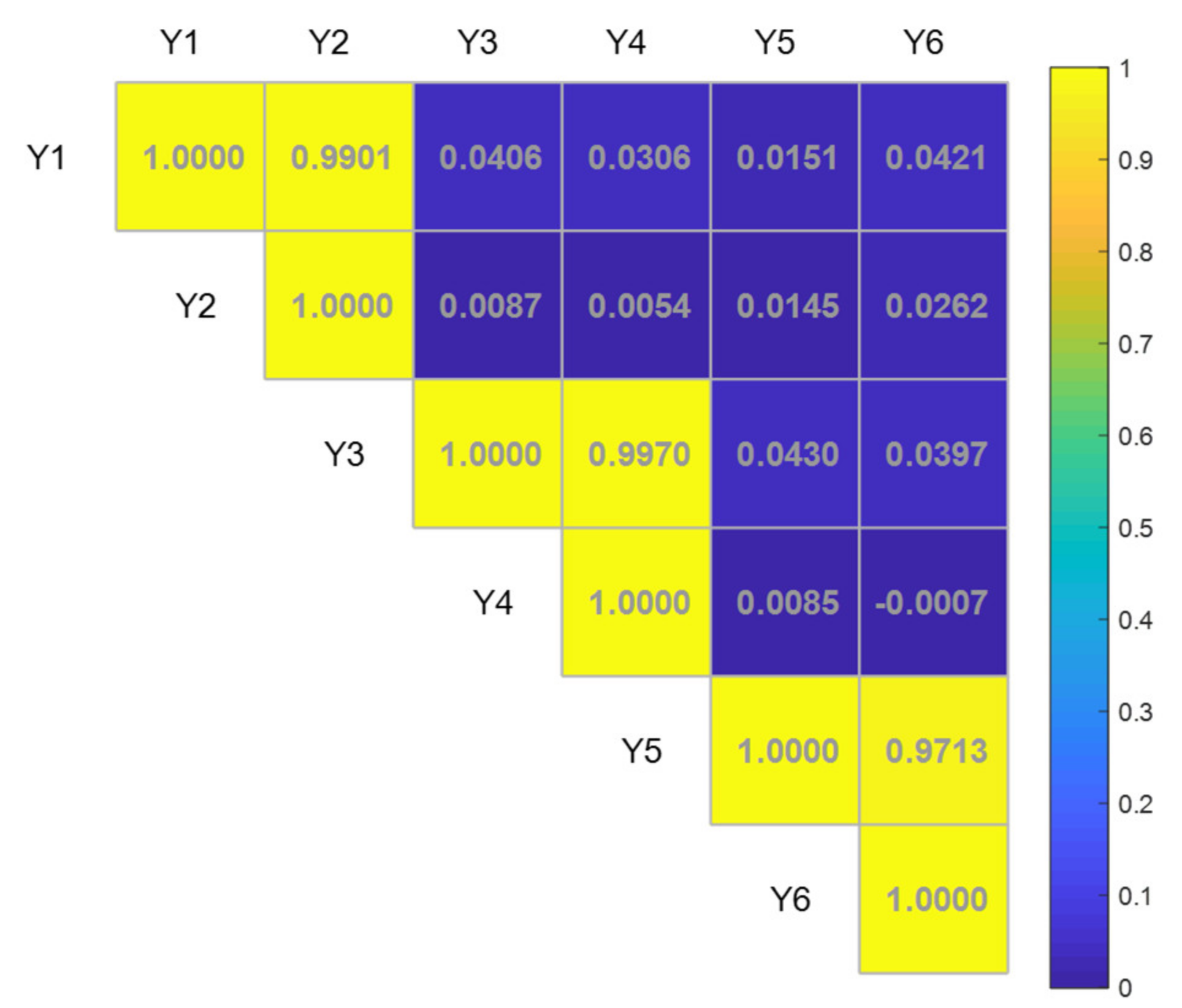
Aiming at the problem of recombination of similar components obtained by using the SGMD algorithm, the cosine similarity is introduced into the SGMD algorithm to obtain the SGMD-CS algorithm. The effectiveness of the method is verified by simulation signals and actual rolling bearing fault signals.

(2)

Based on the SGMD-CS algorithm, SymEn is constructed as the extracted fault feature vector.

(3)

Using Adaboost algorithm to realize automatic identification of bearing failure modes.

(4)

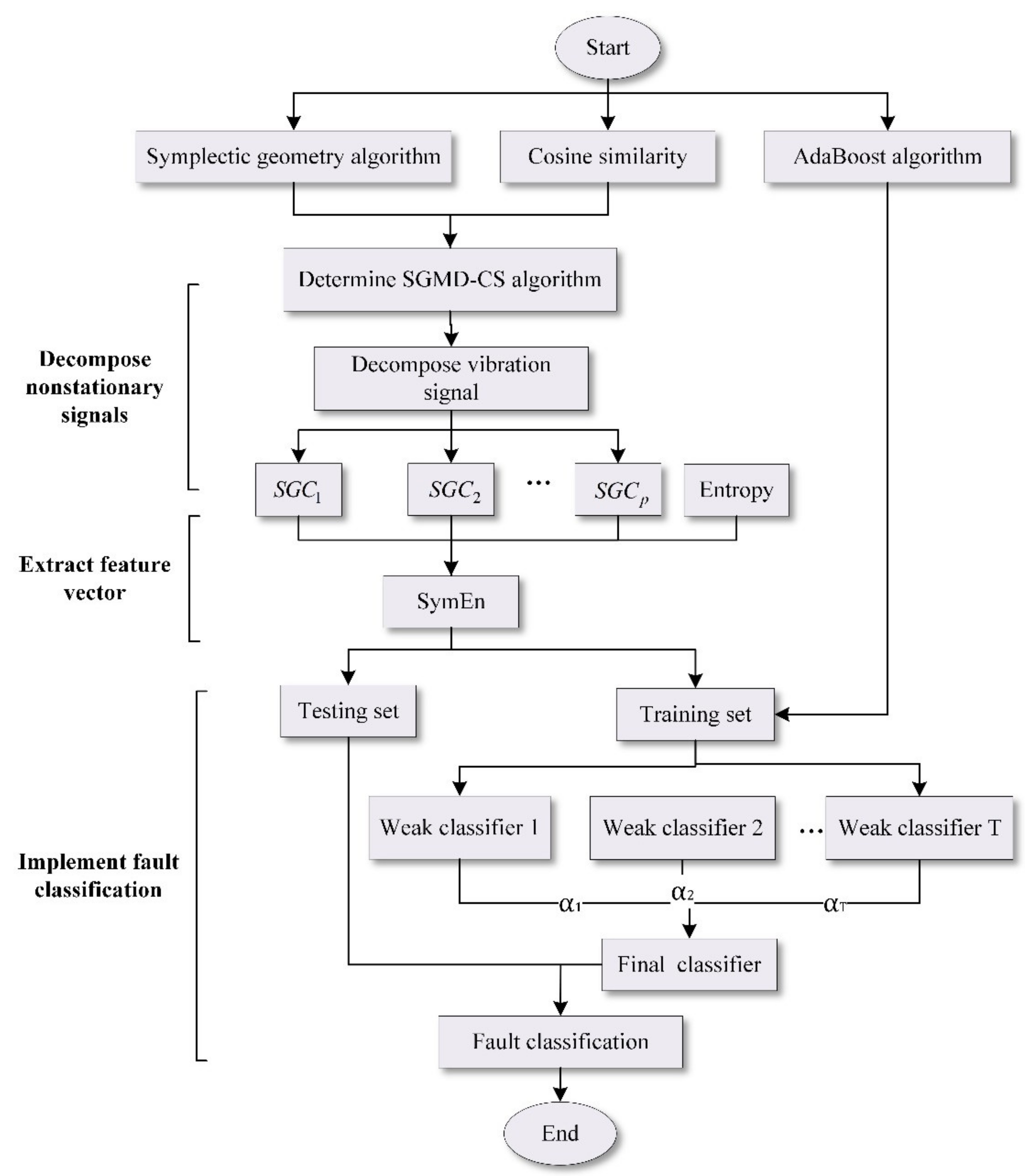
A complete fault diagnosis flowchart of rolling bearings is given, and experimental research and comparative analysis are carried out.

The structure of this paper is as follows: In Section 2, the theoretical part of the symplectic geometry algorithm is introduced, and combining the symplectic geometry algorithm with cosine similarity is discussed. In Section 3, by verifying the simulation signal, the superiority of the SGMD-CS method in terms of signal decomposition is affirmed. In Section 4, we introduce the symplectic geometric entropy and AdaBoost algorithm based on decision trees. In Section 5, we adopt the data of Case Western Reserve University’s Electrical Engineering Laboratory implemented fault diagnosis, highlighting the validity of the proposed method. Finally, in Section 6, we summarize the entire article.

2. Symplectic Geometry Algorithm

The core concept of the symplectic geometry algorithm uses the symplectic matrix to perform QR decomposition to find the eigenvalues of the Hamiltonian matrix. The algorithm is mainly divided into three steps: phase space reconstruction, symplectic QR decomposition, and diagonal averaging transformation. Where, $J=J_{2n}=\left[\begin{array}{cc}0& +I_n\\ -I_n& 0\end{array}\right]$.

2.1. Symplectic Theory

Before introducing the symplectic geometry method, some basic definitions and theorems are given.

Definition 1.

S as a valid matrix; if$JS{J}^{-1}=S^{-T}$, then S is a symplectic matrix.

Definition 2.

H as a valid matrix; if$JH{J}^{-1}=-H^{-T}$, then H is a Hamiltonian matrix.

Theorem 1.

For any symplectic matrix$A_{n\times n}$, a new matrix$M=\left(\begin{array}{cc}A& 0\\ 0& -A^T\end{array}\right)$can be constructed, and M is also a Hamiltonian matrix.

Theorem 2.

Assuming the Household matrix H, where$H=H\left(k,w\right)=\left(\begin{array}{cc}P& 0\\ 0& P\end{array}\right)$, $P=I_n-\frac{2\overline{w}{\overline{w}}^T}{{\overline{w}}^T\overline{w}}$, $\overline{w}={\left(0,\cdots ,0;w_k,\cdots ,w_n\right)}^T\ne 0$, H is a symplectic unitary matrix.

Next, the symplectic geometry method is introduced in detail.

(1)

Phase space reconstruction

For an original time series such as $x=x_1,x_2,\cdots x_n$, $n$ is the length of the signal. Based on Takens embedding theory [28], a one-dimensional signal can be reconstructed into a multidimensional signal by means of the method of delay. Thereby, a trajectory matrix $X$ is constructed, which contains all dynamic information of the time series:

$$X=\left[\begin{array}{cccc}\begin{array}{c}{x}_1\\ ⋮\\ x_m\end{array}& \begin{array}{c}{x}_{1+\tau }\\ ⋮\\ x_{m+\tau }\end{array}& \begin{array}{c}\cdots \\ \\ \cdots \end{array}& \begin{array}{c}{x}_{1+(d-1)\tau }\\ ⋮\\ x_{m+(d-1)\tau }\end{array}\end{array}\right]$$

(1)

where $d$ is the embedding dimension and $\tau$ is the delay time, $n=m+(d-1)\tau$. Obviously, choosing a different embedding dimension and delay time will result in a different trajectory matrix. Here, we refer to the method in [29] to determine the d value by calculating the power spectral density (PSD) of the time series and set $\tau =1$. To be precise, the frequency of the maximum peak is estimated by the PSD method. If the normalized frequency is lower than the given threshold ${10}^{-3}$, d is set to $\frac{n}{3}$; otherwise, the value is set to $d=1.2\times \frac{F_s}{f_{\max }}$, and $F_s$ is the sampling frequency.

(2)

Symplectic QR decomposition

This step is the core of the symplectic geometry method [30].

To obtain the Hamiltonian matrix, the covariance matrix $A$ is first obtained by performing an autocorrelation analysis of the trajectory matrix:

$$A=X^{T}X$$

(2)

Then, the Hamiltonian matrix $M$ will be constructed from matrix $A$:

$$M=\left(\begin{array}{cc}A& 0\\ 0& -A^T\end{array}\right)$$

(3)

It is proven that there is a Householder matrix, $H=\left(\begin{array}{cc}\begin{array}{c}Q\\ 0\end{array}& \begin{array}{c}0\\ Q\end{array}\end{array}\right)$, where the matrix $Q$ can be composed of a real symmetric matrix $A$, and the matrix $H$ is also a symplectic geometric orthogonal matrix. Then:

$$\begin{array}{cc}HM{H}^T& =\left(\begin{array}{cc}Q& 0\\ 0& Q\end{array}\right)\left(\begin{array}{cc}A& 0\\ 0& -A^T\end{array}\right){\left(\begin{array}{cc}Q& 0\\ 0& Q\end{array}\right)}^T\\ & =\left(\begin{array}{cc}QA{Q}^T& 0\\ 0& -Q{A}^T{Q}^T\end{array}\right)\hfill \\ & =\left(\begin{array}{cc}B& 0\\ 0& -B^T\end{array}\right)\hfill \end{array}$$

(4)

where $B$ is an upper Hessenberg matrix, $\left(b_{ij}=0,i>j+1\right)$; it is easy to obtain the following: $\lambda \left(A\right)=\lambda \left(B\right)={\lambda }^2\left(X\right)$.

The eigenvalues of B can be calculated as ${\lambda }_1,{\lambda }_2,\cdots {\lambda }_d$, according to the properties of the Hamiltonian matrix, and the eigenvalues of the matrix $X$ are obtained as:

$${\sigma }_i=\sqrt{{\lambda }_i}\left(i=1,2,\cdots ,d\right)$$

(5)

where ${\lambda }_1>{\lambda }_2>\cdots >{\lambda }_d$, ${\lambda }_i$ in descending order, and the distribution of ${\lambda }_i$ represents the spectral distribution of matrix $A$, where the smaller value is usually considered as the noise components. $Q_i\left(i=1,2,\cdots ,d\right)$ is the eigenvector corresponding to the eigenvalues of matrix $A$, and the transformation coefficient is calculated by the following formula:

$$S_i=Q_i^T{X}^T\left(i=1,2,\cdots ,d\right)$$

(6)

Then:

$$Z_i=Q_i{S}_i\left(i=1,2,\cdots ,d\right)$$

(7)

The corresponding reconstruction matrix $X_i=Z_i^T$ can be obtained, and then trajectory matrix $X$ can be expressed as:

$$X=X_1+X_2+\cdots +X_d$$

(8)

(3)

Diagonal averaging transformation

The dimension of the obtained initial component matrix is m × d. Through diagonal averaging, the reconstruction matrix $X_i$ can be transformed into $d$ sets of time series with length $n$, and the sum of the $d$ sets of time series with length $n$ is the original time series $x$. The specific implementation method is as follows:

For any element $x_{ij}\left(1\le i\le d,1\le j\le m\right)$ in the matrix $X_i$, let $d^{\ast }=\min (m,d)$, $d^{\ast }=\min (m,d)$. If m < d, get $x_{ij}^{\ast }=x_{ij}$; otherwise, $x_{ij}^{\ast }=x_{ji}$ Then the elements $y_k(k=1,2,\cdots ,n)$ in the corresponding time series $Y_i$ are calculated as shown in Equation (9):

$$y_k=\left\{\begin{array}{cc}\frac{1}{k}{\displaystyle \sum _{p=1}^k{x}_{p,k-p+1}^{\ast }}\hfill & 1\le k\le d^{\ast }\\ \frac{1}{d^{\ast }}{\displaystyle \sum _{p=1}^{d^{\ast }}{x}_{p,k-p+1}^{\ast }}\hfill & d^{\ast }\le k\le m^{\ast }\\ \frac{1}{n-k+1}{\displaystyle \sum _{p-k-m^{\ast }+1}^{n-m^{\ast }+1}{x}_{p,k-p+1}^{\ast }}\hfill & \hspace{1em}{m}^{\ast }<k\le n\end{array}\right.$$

(9)

Based on Formula (9), the matrix $X_i$ is converted into a series of $Y_i(y_1,y_2,\cdots ,y_n)$. Therefore, through diagonal averaging, we can transform the trajectory matrix $X$ into a series of length $n$:

$$Y=Y_1+Y_2+\cdots +Y_d$$

(10)

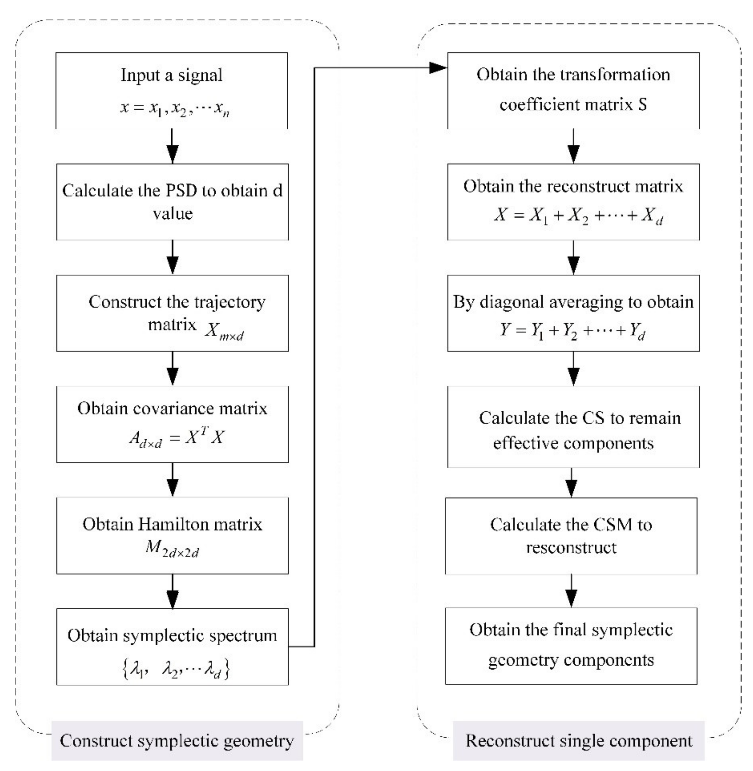
2.2. SGMD-CS Algorithm

During the decomposition of symplectic geometric models, we have obtained $\left\{Y_1,Y_2,\dots ,Y_d\right\}$; in these d sets of initial components, some components may have the same periodic component, frequency component, and characteristics. Therefore, these components are not completely independent of each other, and these initial components with the same characteristics need to be reconstructed by other methods. This paper introduces cosine similarity here during the reconstruction process. The definition is as follows:

$$Y_{ij}=\cos {\theta }_{ij}=\frac{Y_i\cdot Y_j}{‖Y_i‖\cdot ‖Y_j‖} 1\le \mathrm{i}\le d,1\le j\le d$$

(11)

Due to the interference of environmental factors, the signal often contains many noise components, so we should separate the useful components from the noise components. The specific method is as follows:

First, the noise components are separated. In the previous step, we can obtain d sets of initial components, and the new $d$ sets of constructed components $N_f={\displaystyle {\sum }_{i=1}^f{Y}_i\left(f=1,2,\cdots ,d\right)}$ can be obtained by adding the first $f$ sets of components. By calculating the cosine similarity $N_{k,k+1}=\cos {\theta }_{{}_{k,k+1}}=\frac{N_k\cdot N_{k+1}}{‖N_k‖\cdot ‖N_{k+1}‖}\left(k=1,2,\cdots d-1\right)$ of two adjacent constructed components, when the value of the cosine similarity reaches a threshold and changes slowly, it can be approximated that the threshold corresponding to the demarcation point $k$ is a turning point for reconstructing the effective components. Before this point, the component contains most of the information of the original signal, which should be retained for subsequent analysis; after this point, it can be regarded as noise. Second, the remaining effective $k$ sets of components are recombined between similar components. By constructing a cosine similarity matrix, similar components are combined to determine the final symplectic geometric components. The cosine similarity matrix constructed is as follows:

$$CSM=\left[\begin{array}{cccc}1& Y_{12}& \dots & Y_{1k}\\ Y_{21}& 1& \dots & Y_{2k}\\ ⋮& ⋮& \dots & ⋮\\ Y_{k1}& Y_{k2}& \cdots & 1\end{array}\right]$$

(12)

Obviously, the cosine similarity matrix (CSM) is a symmetric matrix, and the diagonal elements are all the same. Through this matrix, the components with higher similarity are recombined.

In summary, the flowchart of the SGMD-CS algorithm is shown in Figure 1.

3. Simulation Analysis

To verify the effectiveness of the proposed method, we refer to paper [20] to construct the complex amplitude modulation and frequency modulation signal to verify the SGMD-CS method. The constructed simulation signal is shown as Equation (13):

$$\left\{\begin{array}{c}{x}_1(t)=2\sin (60\pi t)\times (1+0.5\sin (2\pi t))\hfill \\ x_2(t)=\sin (120\pi t)\hfill \\ x_3(t)=0.5\cos (10\pi t)\hfill \\ x(t)=x_1(t)+x_2(t)+x_3(t)\hfill \end{array}\right.$$

(13)

$x\left(t\right)$ includes an amplitude modulation and frequency modulation component, a sine component, and a cosine component. The time-domain waveform of the simulation signal is shown in Figure 2a, and the frequency-domain waveform of the simulation signal is shown in Figure 2b:

Using the proposed SGMD-CS method to decompose the simulation signal, the decomposition results are shown in Figure 3.

Here, taking the decomposition of the simulation signal as an example, each parameter in the decomposition process is explained. First, for the given simulation signal, we set the sampling frequency to 1000 and convert it into an original time series with a length of 1000. By calculating the power spectral density, $f_{\max }$ is estimated to be 29.7852, so the value of d is equal to 40. That is, after a series of transformations, 40 sets of initial components are finally decomposed. We need to reorganize the 40 sets of initial components with similar characteristics. To reduce the amount of calculation, we need to construct the signals $N_f={\displaystyle {\sum }_{i=1}^f{Y}_i\left(f=1,2,\cdots ,40\right)}$ and calculate the cosine similarity $\cos {\theta }_{{}_{k,k+1}}\left(k=1,2,\cdots 39\right)$ of two adjacent constructed signals, which is shown in Figure 4. It can be seen that $\cos {\theta }_{{}_{k,k+1}}=1\left(k\ge 6\right)$, $\cos {\theta }_{6,7}=1$ shows that the information between $N_6$ and $N_7$ is similar roughly. In other words, the information contained in the sum of the first 6 sets of components can be regarded that they already contain most of the information of the original series. So, the demarcation point $k=6$ is a turning point for reconstructing the effective components, only the first 6 components need to be reconstructed.

Next, component reconstruction is performed by constructing a cosine similarity matrix for the first six components. Since the elements in the matrix represent the similarity between any two components, it is a symmetric matrix. For simplicity, only the elements above the main diagonal are listed. The color block diagram drawn according to the cosine similarity matrix is shown in Figure 5.

It can be clearly seen from Figure 5 that the cosine similarity of the first component and second component is 0.9901, which can be considered that the two components are similar, and they are reorganized as $SG{C}_1$. Similarly, the cosine similarity between the third component and the fourth component is 0.9970, and they are regrouped into $SG{C}_2$. The fifth component and the sixth component, with a similarity of 0.9713, are recombined into $SG{C}_3$. The final decomposed components are shown in the first three waveforms of Figure 3. The fourth waveform represents the remaining component, that is, the sum of the initial components from the seventh to the fortieth component. The sum of these four parts is equal to the original simulated signal.

For comparison, the constructed simulation signals are decomposed with the LMD and EMD algorithms. The results of the decomposition are shown in Figure 6 and Figure 7.

Decomposing the simulation signal by these three methods and comparing the obtained time-domain and frequency-domain waveforms, it can be seen that the SGMD-CS method can separate the trend components of the original simulation signal very well, and the components of the decomposition are almost equivalent to the components of the original signal. There is no doubt that the decomposition result is quite good. Moreover, the LMD method decomposes the original simulated signal into four components. It can be clearly seen in Figure 5 that the components $P{F}_1$ and $P{F}_2$ produce modal aliasing. The 30 Hz and 60 Hz components appear simultaneously in $P{F}_1$; this situation is called under-decomposition. In addition, the 30 Hz component appears in $P{F}_1$ and $P{F}_2$, and the 5 Hz component appears in $P{F}_2$ and $P{F}_3$; this situation is called over-decomposition. We can also find that the amplitude of some components is reduced, so the decomposition result is not ideal compared to the previous method. Similarly, the EMD method is used to decompose the simulated signal, and the decomposition result is shown in Figure 6. It can be seen that the decomposition obtains 8 components. Similar to LMD, under-decomposition and over-decomposition also occur during the decomposition process, and the decomposition result is not ideal. After analysis, regardless of whether the LMD or EMD is used, these two methods are not as effective as the SGMD-CS method for decomposing the simulation signal.

To further verify the similarity between the components decomposed by the SGMD-CS method and the components of the original simulated signal, the waveforms decomposed by the two approaches are drawn in Figure 8. It can be seen from the figure that the error of the decomposition result is smaller when using the proposed method, so this method can better strip the trend components of the complex signals. Therefore, in the wind turbine fault diagnosis process, the SGMD-CS method is first used to decompose the vibration signal collected by the sensor, thereby extracting the fault information hidden in the original signal, providing necessary materials for subsequent fault diagnosis, and improving the accuracy of fault diagnosis correspondingly.

4. Feature Classification

4.1. AdaBoost Theory

Boosting, as a meta-algorithm framework, is an important integrated learning technique that can reinforce weak learning classifiers, whose prediction accuracy is only slightly higher than that of random guessing, into strong predictors with high prediction accuracy. These weak classifiers can be any classifiers, such as decision trees, simple linear logistic classifiers, simple SVM classifiers, etc. This approach has been successfully applied to solve problems such as object detection, text analysis, and data mining. The most widely used boosting algorithm is AdaBoost, which was proposed by Freund and Schapire in 1996 [31]. As one of the best-supervised classification algorithms, it has been widely used to solve complex classification problems because of its simple concept [32,33].

Considering decision trees are resistant to overfitting since trees often have large edges and limited complexity, therefore, in this paper, we choose decision trees as the basic classifiers [34].

The specific algorithm steps are as follows:

• Step 1: Calculate the input.

  (1)

  Given training set $\left(x_1,y_1\right),\cdots \left(x_m,x_m\right)$, where $x_i\in X,y_i\in \left\{-1,+1\right\}$.

  (2)

  Weak learning algorithm.

• Step 2: Calculate the output $H_{final}\left(x\right)$.

  (1)

  Initial weight distribution of training data.

  $$D_1\left(i\right)=\frac{1}{m}\left(\forall i\right), i=1,2,\cdots ,m$$

  (14)

  (2)

  For $t=1,\cdots ,T$, using the training data set with weight distribution $D_t$ to learn, we obtain a weak classifier.

  $$h_t(x):X\to \left\{-1,+1\right\}$$

  (15)

  (3)

  Calculate the classification error rate on the training data set $h_t\left(x\right)$.

  $${\epsilon }_t={\mathrm{Pr}}_{i~D_t}\left[h_t(x_i)\ne y_i\right]$$

  (16)

  (4)

  Calculate the coefficient of $h_t\left(x\right)$.

  $${\alpha }_t=\frac{1}{2}\ln (\frac{1-{\epsilon }_t}{{\epsilon }_t})$$

  (17)

  It is worth noting that ${\alpha }_t>0$.

  (5)

  Update the weight distribution of the training data set.

  $$\begin{array}{ll}{D}_{t+1}(i)=& \frac{D_t(i)}{Z_t}\times \left\{\begin{array}{c}{e}^{-{\alpha }_t} if y_i=h_t(x_i) \\ e^{{\alpha }_t} if y_i\ne h_t(x_i)\end{array}\right.\\ & =\frac{D_t(i)}{Z_t}\exp (-{\alpha }_t{y}_i{h}_t(x_i) )\hfill \end{array}$$

  (18)

  where $Z_t$ is the normalization factor.

  (6)

  Construct a linear combination of basic classifiers to obtain the final classifier.

  $$H_{\mathrm{final}}(x)=sign\left({\displaystyle \sum _t{\alpha }_t{h}_t(x)}\right)$$

  (19)

4.2. Feature Vector Selection

To obtain as much fault information as possible and improve the accuracy of fault diagnosis, many scholars have excelled in extracting feature vectors, trying to extract the fault features from various angles. Multidimensional feature vectors are selected frequently; however, due to the redundant information, the accuracy of fault diagnosis is reduced, which has forced scholars to seek various dimensionality reduction methods to further handle the selected feature vectors. Literature [35] extracted the fault information in the time domain, frequency domain, and time-frequency domain and then reduced the data through PCA to extract the fault features more comprehensively and realize the accurate identification of faults. In this article, unlike the concepts adopted by previous scholars, we do not consider how to select multidimensional feature vectors. Instead, we consider whether we can choose low-dimensional feature vectors to achieve a similar effect. This places higher requirements on choosing the feature vectors.

Here, we adopt entropy to construct a low-dimensional feature vector. Entropy can usually be used to describe and quantify the degree of confusion in the system. At present, there are many estimation methods about entropy, such as approximate entropy, sample entropy, fuzzy entropy, etc., and they are widely used in various fields to measure the complexity of time series [36,37,38]. In this paper, calculate the symplectic geometric entropy by combining the SGMD-CS algorithm proposed above with the entropy, and select this index as the feature vector. The specific implementation steps are as follows: first, decompose the collected signal. Then, select the first two components decomposed to calculate the corresponding symplectic geometric entropy. Finally, the two-dimensional feature vector $SymEn=\left[e_1,e_2\right]$ is input into the subsequent classifier for fault classification and recognition.

In the second section, we introduced the symplectic geometry algorithm. Through this algorithm, the eigenvalues of the real symmetric matrix $A$ constructed by the trajectory matrix $X$ can be obtained, and the values of ${\lambda }_1,{\lambda }_2,\cdots ,{\lambda }_d$ decrease in sequence. The distribution of ${\lambda }_i$ represents the spectral distribution of matrix $A$. Then, the probability of energy distribution in different directions can be defined as $p_1,p_2,\cdots p_d$, which are calculated as follows:

$$p_i=\frac{{\lambda }_{\mathrm{i}}}{{\displaystyle \sum _{i=1}^d{\lambda }_i}}$$

(20)

where $d$ is the embedding dimension, $0\le p_i\le 1$, ${\displaystyle \sum _{i=1}^d{p}_i=1}$, and $p_i$ describes the uncertainty of entropy in different directions.

Then, the symplectic geometric entropy can be defined as follows:

$$SymEn=-{\displaystyle \sum _{i=1}^d{p}_i}\log (p_i)$$

(21)

Through formula (20) and formula (21), we can calculate symplectic geometric entropy as a feature vector to characterize the fault information. Finally, Figure 9 shows the complete fault diagnosis process.

5. Experimental Analysis

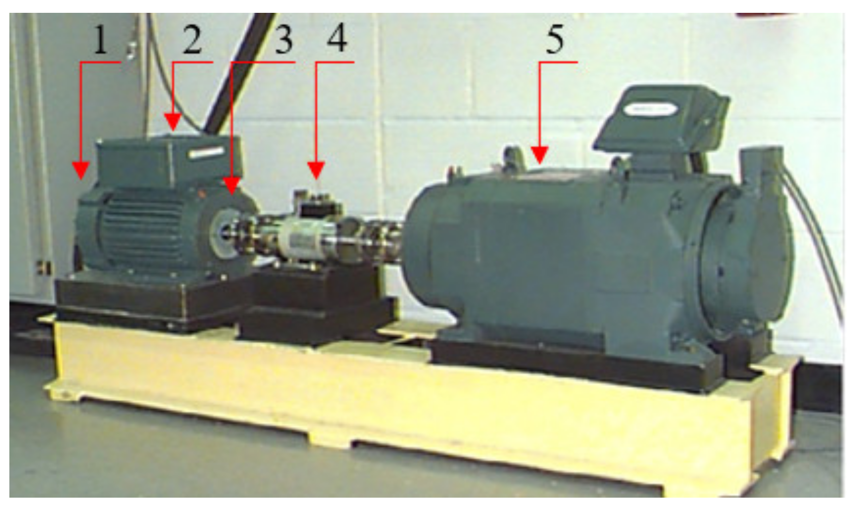
5.1. Experimental Arrangement and Data Description

In this paper, the vibration data of rolling bearings at the Electrical Engineering Laboratory of Case Western Reserve University are selected, and the experimental platform is shown in Figure 10. Motor bearings were seeded with faults using electro-discharge machining (EDM). Faults ranging from 0.007 inches in diameter to 0.021 inches in diameter were introduced separately at the inner raceway, rolling element (i.e., ball), and outer raceway. The specifications of the rolling bearing tested in the experiment and related characteristic frequencies are shown in

Table 1. Bearing specifications.

Class	Deep Groove Ball Bearing
Type	6205-2RS JEM SKF
Position	Drive end
Sampling frequency fs (Hz)	12,000
Inside diameter (inches)	0.9843
Outside diameter (inches)	2.0472
Thickness (inches)	0.5906
Ball diameter (inches)	0.3126
Pitch diameter (inches)	1.537
Rotation frequency (Hz)	$f_r$
Inner ring defect frequency $f_i$ (Hz)	5.4152 × fr
Outer ring defect frequency $f_o$ (Hz)	3.5848$\times f_r$
Rolling element frequency $f_b$ (Hz)	4.7135$\times f_r$
Number of rolling elements	9

.

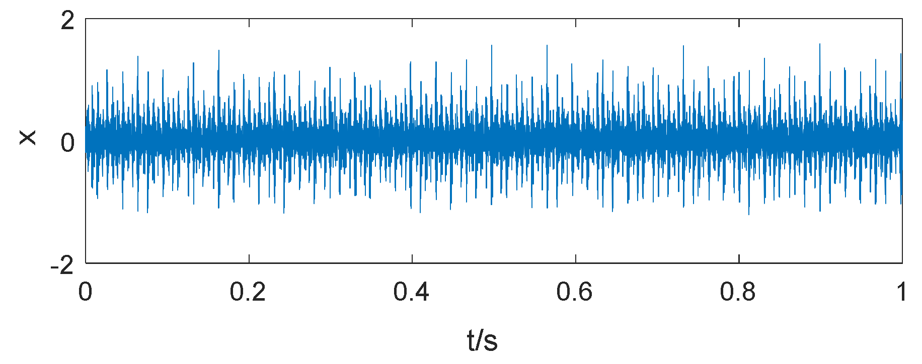
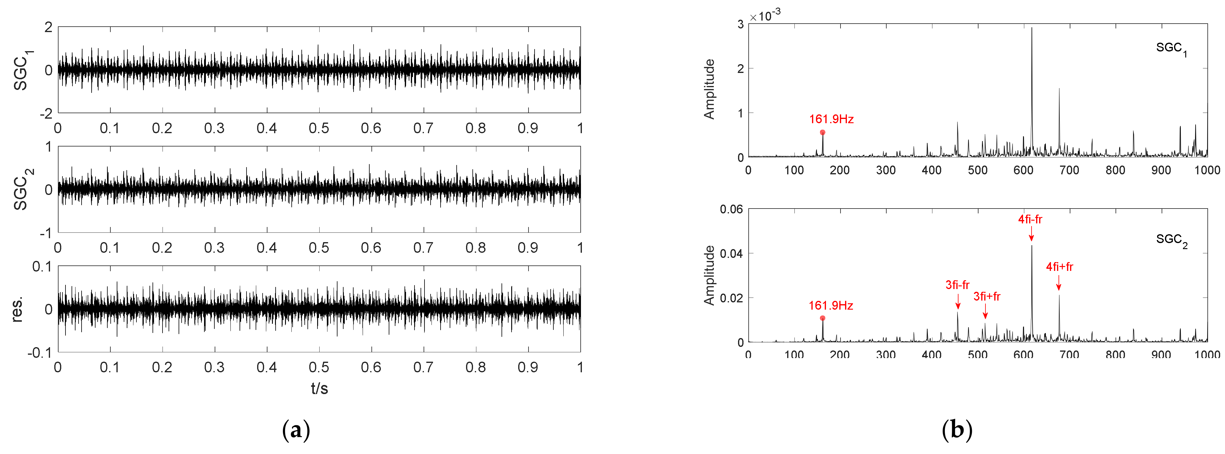
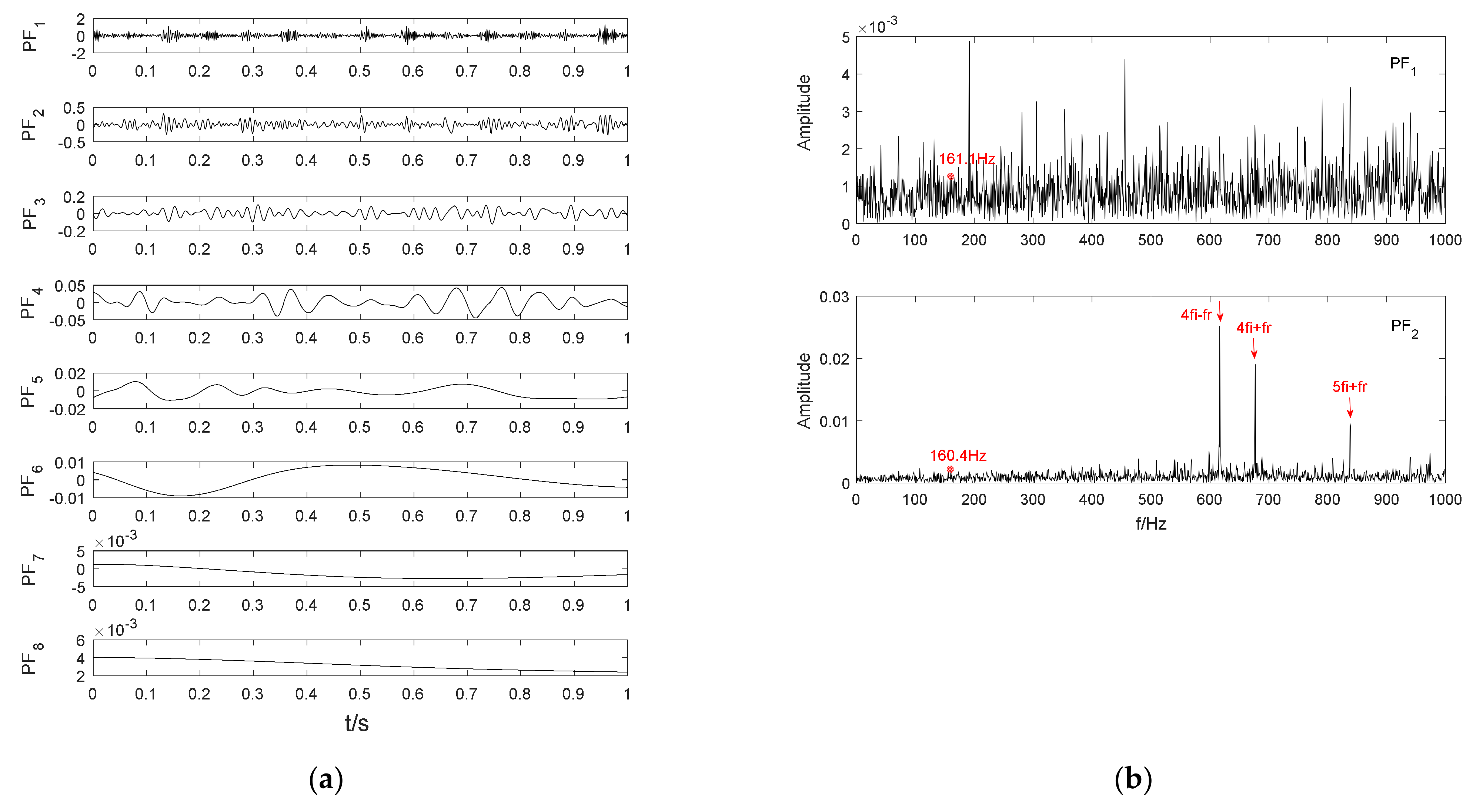
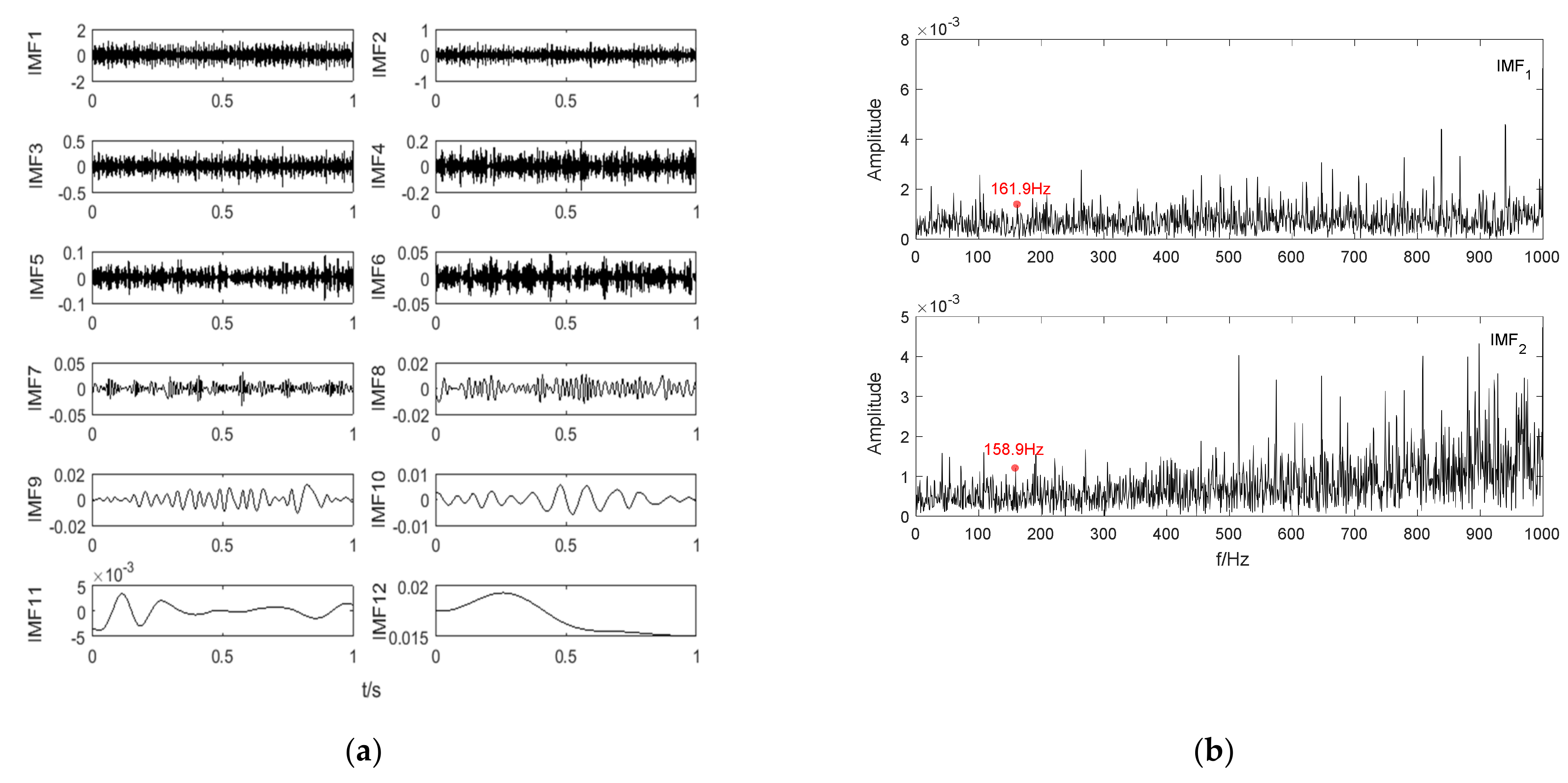
5.2. Signal Preprocessing

The proposed SGMD-CS method is applied to actual rolling bearing signals to prove its effectiveness and feasibility, so it can be used to realize the fault diagnosis of wind turbine bearings. The specific technical parameters of the analyzed bearing are shown in

Table 2. the specific technical parameters of analyzed bearing.

Parameters	Value
Data	105.mat
Fault diameter	0.007″
Approximate motor speed	1797 rpm
Rotation frequency	29.95 Hz
Inner ring defect frequency	162.19 Hz
Motor load	0 hp

. Extract 12,000 data points for analysis.

The time-domain waveform of the analyzed inner ring fault rolling bearing signal is shown in Figure 11. It is decomposed by the SGMD-CS method, and the first two symplectic geometric components are spectrum analyzed, as shown in Figure 12. Taking the amplitude spectrum of $SG{C}_2$ as an example, the spectrum line at 161.9 Hz can be clearly seen from the figure. Because 161.9 Hz is close to the theoretical value 162.19 Hz, which is the inner ring fault frequency of rolling bearing, it can be considered that the inner ring fault has been identified. In addition, the sidebands of the high-order harmonics of the inner ring fault frequency are prominent and can be clearly observed, whose amplitude are modulated by $f_r$.

For comparison, the LMD and EMD methods are used to process the fault signal in the same way. The decomposition results are shown in Figure 13 and Figure 14. It can be seen from the figure that there are so many interference components with large amplitude that the characteristic frequency of the fault is almost submerged in the noise signal. Characteristic frequency cannot be accurately identified, which brings certain difficulties to the judgment of the fault of the rolling bearing.

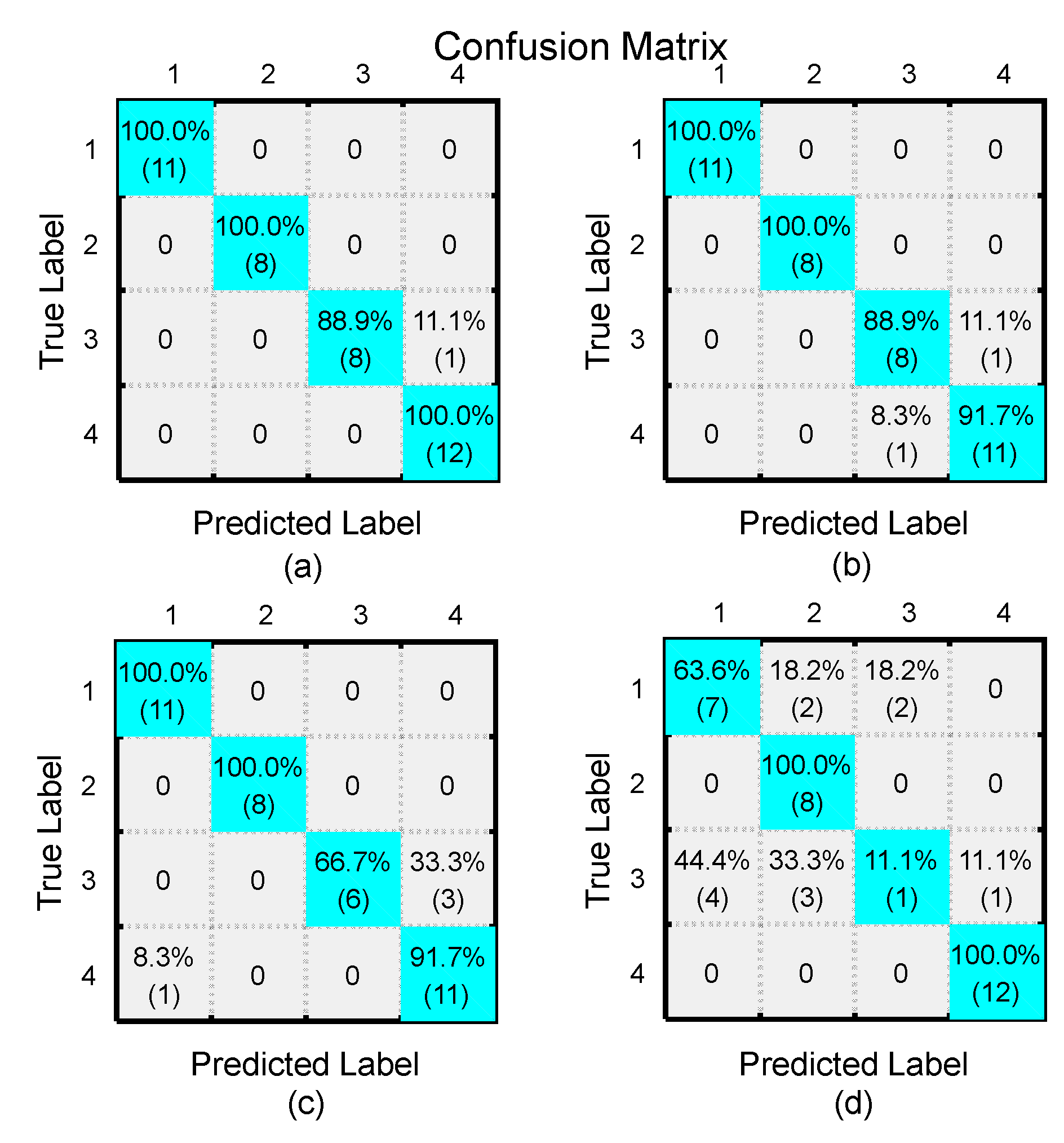
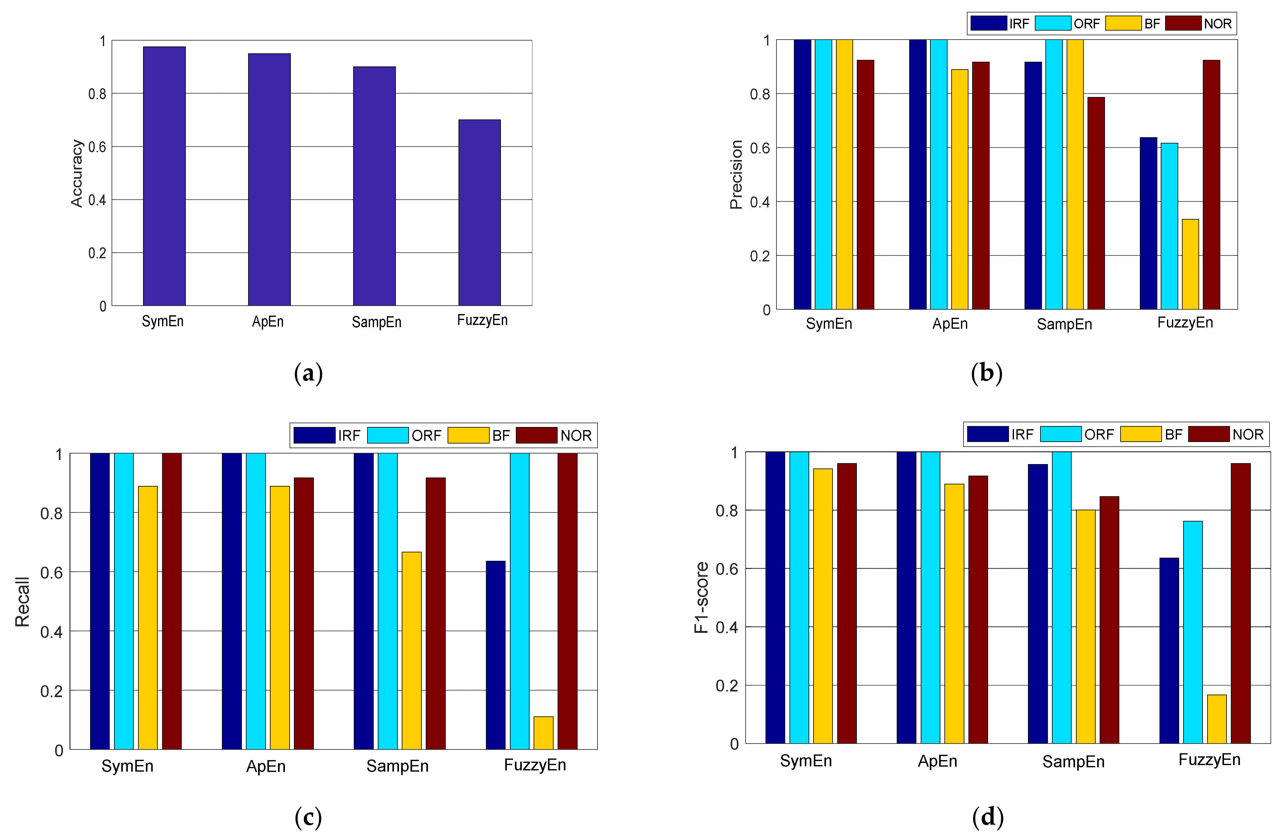
5.3. Classification of Different Fault Types

In the previous section, a series of comparative experiments were conducted to verify the effectiveness of the proposed SGMD-CS method for processing rolling bearing fault signals. According to the flow chart of fault diagnosis process shown in Figure 8, this method is combined with machine learning to realize the intelligent diagnosis of bearing faults.

In order to classify the different fault categories of the bearing, the original vibration signal data of each fault type is taken to intercept the first 50 windows, each window contains 1024 points, so as to obtain 50 fault samples for every type of fault. For each sample, the SGMD-CS method is used to decompose, the first two SGC components are selected for analysis, and the symplectic geometric entropy is calculated. Therefore, for four different fault types, the entire data set contains 200 samples, and the classification accuracy is verified by the five-fold cross-validation method. At the same time, in order to verify the validity of the symplectic geometric entropy as the extracted feature, approximate entropy, sample entropy, and fuzzy entropy are used for comparison. The specific data set description is shown in

Table 3. Description of experimental dataset.

Fault Type	Data	Fault Diameter (Inches)	Motor Load (HP)	Rotation Frequency (r/min)	Class Label
Inner ring fault (IRF)	171.mat	0.014	2	1750	1
Outer ring fault (ORF)	199.mat	0.014	2	1750	2
Ball element fault (BF)	187.mat	0.014	2	1750	3
Normal (NOR)	099.mat	0.014	2	1750	4

.

Take one of the experiments as an example for specific analysis. Figure 15 shows the classification results of the model for different extracted feature vectors in the form of a confusion matrix. For the classification model that uses symplectic geometric entropy as the feature vector, the classification accuracy rate is 97.5%, and one misjudgment occurs because the rolling element fault is misjudged as normal. In terms of the approximate entropy is used as the feature vector, the classification accuracy rate is 95%, 2 misjudgments occur between the rolling element fault and the normal state. Using sample entropy as the feature vector model, the classification accuracy rate is 90%. There are 4 misjudgments, and 3 misjudgments are relevant to rolling element fault. For the model that uses fuzzy entropy as the feature vector, the classification accuracy rate is only 70%, and there are 12 misjudgments, of which 8 misjudgments are related to the rolling element fault. To evaluate the performance of the classifier only from the index of accuracy, it can be considered that the symplectic geometric entropy as the extracted fault feature has a certain validity, while the fuzzy entropy calculated as the extracted fault feature under this condition performs poorly. In addition, we can also find that most of the misjudgments are related to the rolling element fault.

In order to comprehensively evaluate the classification effect of different models, four common evaluation indicators are used as shown in Figure 16. They are accuracy, precision, recall, and F1-score. Based on the four indicators, it is not difficult to draw the same conclusion as the previous one, that is, extracting the symplectic geometric entropy of the bearing vibration signal as a feature vector is extremely superior and more stable. The specific values of each evaluation index are shown in

Table 4. Result of classification.

		SymEn	ApEn	SampEn	FuzzyEn
	Accuracy	97.50	95.00	90.00	70.00
	Precision	100.00	100.00	91.67	63.64
Inner ring	Recall	100.00	100.00	100.00	63.64
	F1-score	100.00	100.00	95.65	63.64
	Precision	100.00	100.00	100.00	61.54
Outer ring	Recall	100.00	100.00	100.00	100.00
	F1-score	100.00	100.00	100.00	76.19
	Precision	100.00	88.89	100.00	33.33
Ball element	Recall	88.89	88.89	66.67	11.11
	F1-score	94.12	88.89	80.00	16.67
	Precision	92.31	91.67	78.57	92.31
Normal	Recall	100.00	91.67	91.67	100.00
	F1-score	96.00	91.67	84.62	96.00

.

Similarly, the comparative results of other experiments are analyzed to avoid obvious deviations in a single experiment. In all experiments, calculate the mean and standard deviation of the experimental results under different evaluation standards, as shown in

Table 5. Result of statistics.

		SymEn	ApEn	SampEn	FuzzyEn
	Accuracy	93.00 ± 5.12	91.00 ± 4.54	88.50 ± 7.83	67.50 ± 3.95
	Precision	89.67 ± 10.83	88.14 ± 11.39	88.14 ± 11.39	51.90 ± 21.18
Inner ring	Recall	100.00 ± 0.00	97.78 ± 4.97	97.78 ± 4.97	49.83 ± 14.68
	F1-score	94.27 ± 6.13	92.32 ± 7.08	92.32 ± 7.08	49.21 ± 13.09
	Precision	96.00 ± 8.94	96.57 ± 4.80	93.70 ± 8.80	69.31 ± 13.17
Outer ring	Recall	92.35 ± 8.39	92.57 ± 12.99	96.57 ± 4.80	88.70 ± 7.29
	F1-score	94.08 ± 8.27	93.99 ± 7.24	94.88 ± 5.09	76.88 ± 7.74
	Precision	88.95 ± 12.08	85.99 ± 14.17	86.48 ± 16.34	50.33 ± 17.89
Ball element	Recall	88.82 ± 10.58	77.10 ± 15.24	67.84 ± 25.46	36.72 ± 21.71
	F1-score	88.71 ± 10.31	80.52 ± 12.79	74.57 ± 21.12	41.10 ± 20.40
	Precision	98.46 ± 3.44	94.40 ± 5.48	85.48 ± 11.12	98.46 ± 3.44
Normal	Recall	89.27 ± 6.67	95.83 ± 5.89	90.00 ± 10.87	92.35 ± 7.48
	F1-score	93.43 ± 2.20	95.09 ± 5.45	87.44 ± 9.99	95.10 ± 3.37

. On the whole, the accuracy of model that uses symplectic geometric entropy as the feature vector is the highest, followed by approximate entropy and sample entropy, and the accuracy of fuzzy entropy is the lowest. Other evaluation criteria also roughly conform to this law. And no matter which evaluation standard is used, the value of rolling element fault is lower than that of the other three fault types, so it is prone to misjudgment. Even under this kind of unfavorable conditions, the symplectic geometric entropy still has advantages than the other three types of entropy, reflecting its advantages in feature extraction.

The above experimental results show that the wind turbine fault feature extraction method based on the SGMD-CS and AdaBoost framework proposed in this paper is correct and effective, which has a certain significance for the bearing fault identification of wind turbines and then provide a corresponding basis for a technician to carry out maintenance work.

6. Conclusions

This paper proposes a fault feature extraction method for wind turbines based on the SGMD-CS and AdaBoost framework, which has been improved and optimized as follows:

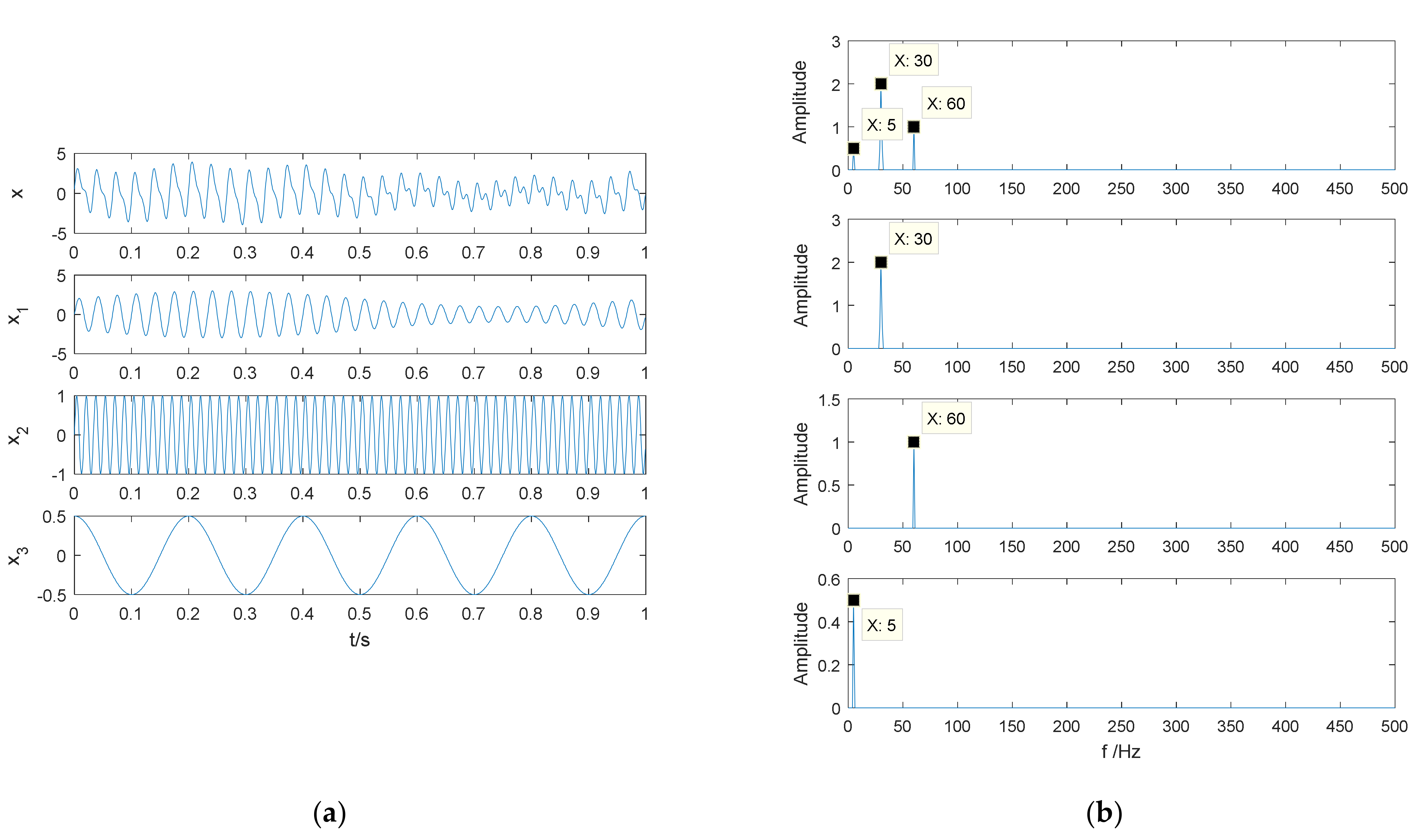
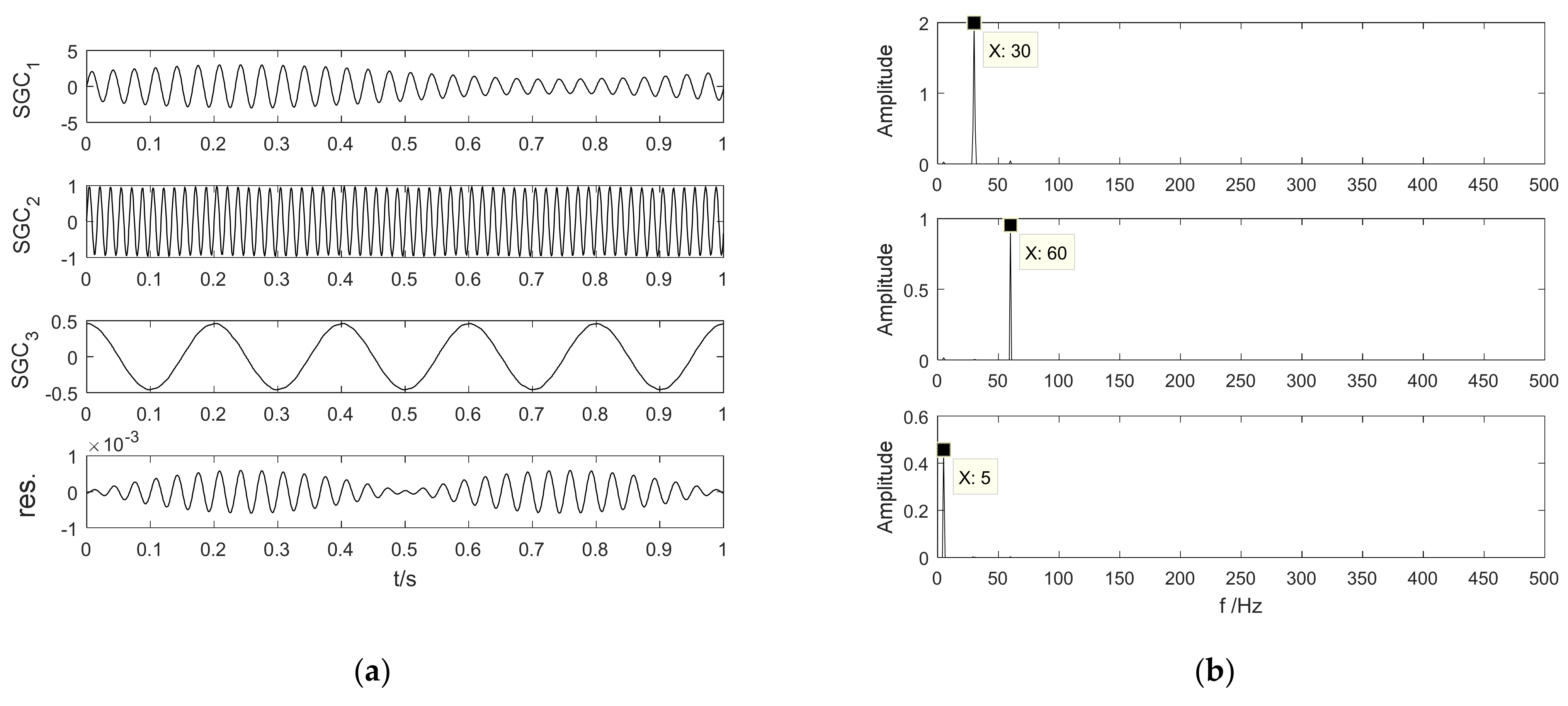
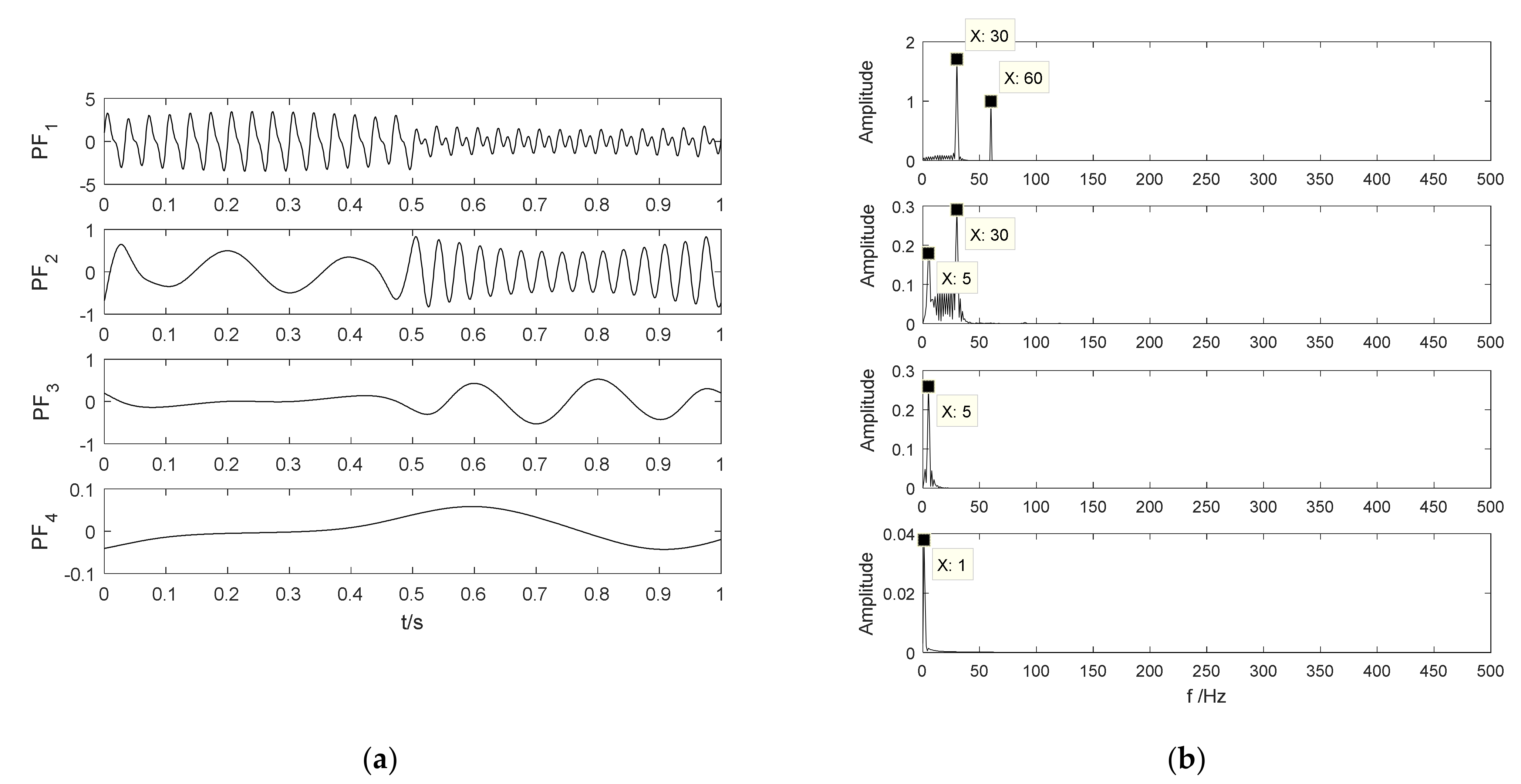
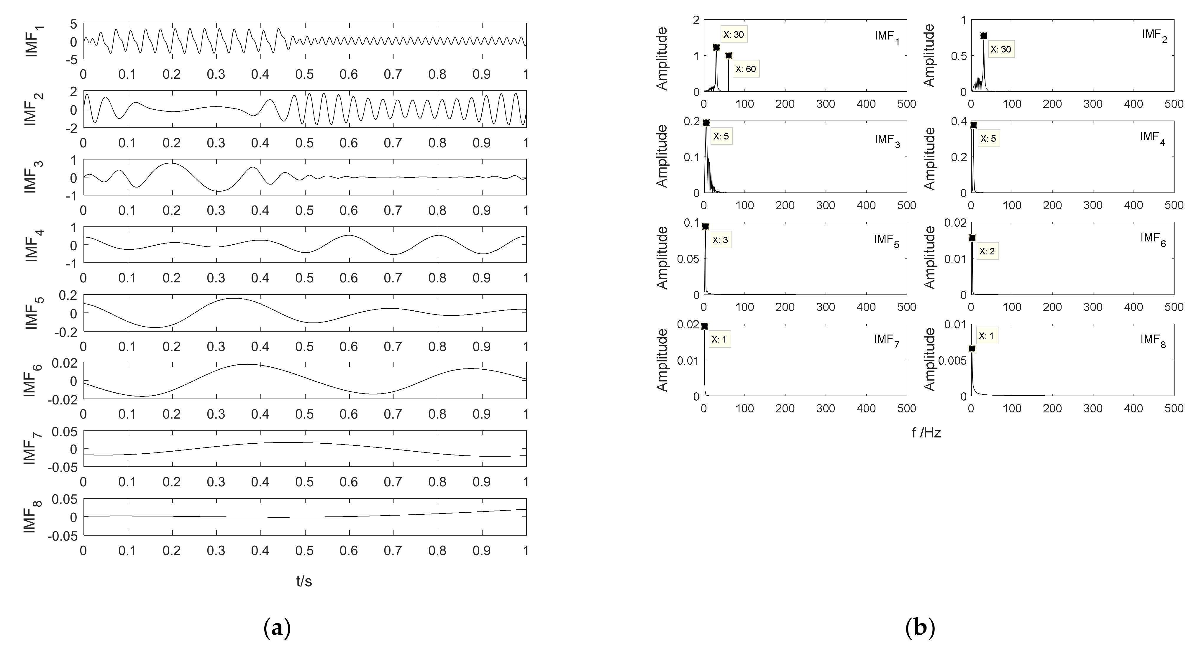
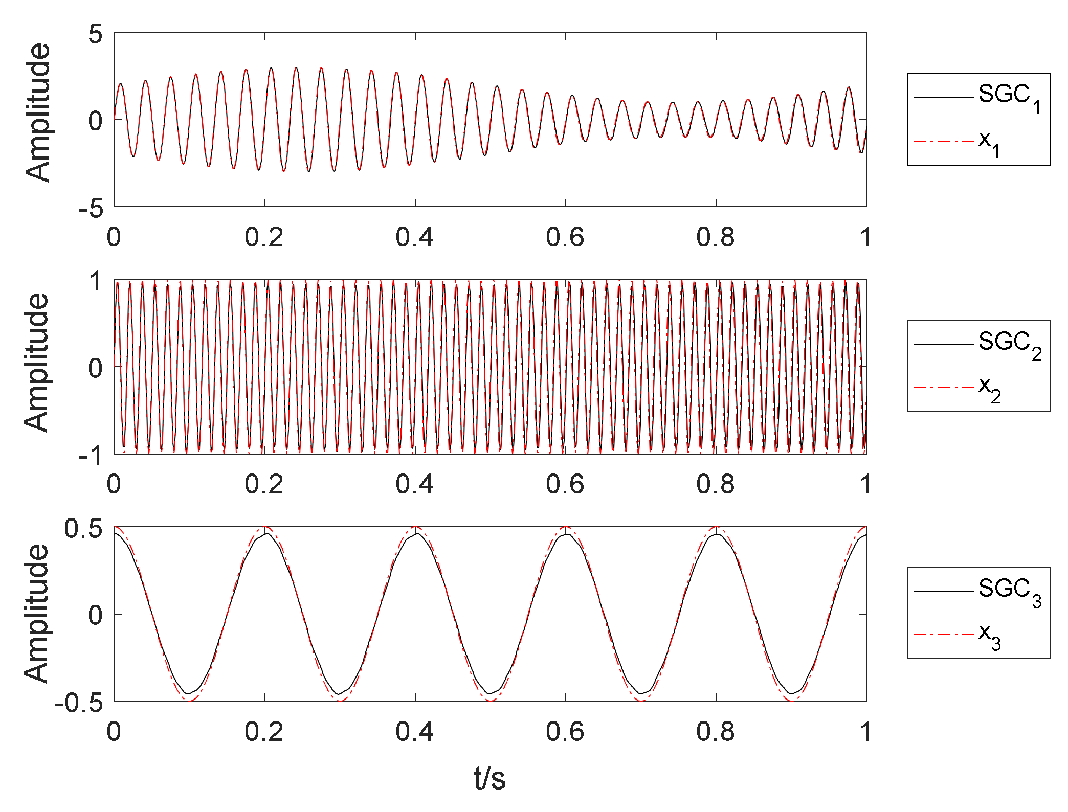
• To address the problem of similar component recombination in the symplectic geometric decomposition process, the cosine similarity is introduced into this method, the SGMD-CS method is proposed, and a block diagram of the method is given. The effectiveness of this method is verified by constructing a complex AM-FM signal and comparing it with the decomposition results of the LMD and EMD methods. The results show that the decomposition error of this method is small, and the trend components of the original signal can be better stripped, so this method is suitable for the analysis of nonlinear time series. In addition, the characteristics of this method have also been compared and verified on actual rolling bearing fault signals.
• When addressing the problem of using high-dimensional feature vectors when extracting fault feature information, there will be data redundancy, and the diagnosis accuracy will be reduced. In this paper, based on the SGMD-CS method, the symplectic geometric entropy is calculated as a low-dimensional feature vector and sent to the AdaBoost classification framework based on decision trees. According to the given fault diagnosis flow chart, taking the rolling bearing vibration data of Case Western Reserve University’s Electrical Engineering Laboratory as an example, a high classification accuracy rate is obtained by discriminating and classifying the fault type. At the same time, compared with sample entropy, approximate entropy, and fuzzy entropy, symplectic geometric entropy is highlighted as a measure that can effectively extract fault information, thereby making the diagnosis more accurate.

References

1. Liu, Z.; Zhang, L. A review of failure modes, condition monitoring and fault diagnosis methods for large-scale wind turbine bearings. Measurement 2020, 149, 107002. [Google Scholar] [CrossRef]
2. Ehsan, M.; David, W.; Qiao, S. Indicative Fault Diagnosis of Wind Turbine Generator Bearings Using Tower Sound and Vi-bration. Energies 2017, 10, 1853. [Google Scholar]
3. Francesco, C.; Luigi, G.; Alessandro, P.D.; Davide, A.; Francesco, N. Diagnosis of Faulty Wind Turbine Bearings Using Tower Vibration Measurements. Energies 2020, 13, 1474. [Google Scholar]
4. Daniel, S.; Pär, M.; Kim, B.; Per-Erik, L. Bearing monitoring in the wind turbine drivetrain: A comparative study of the FFT and wavelet transforms. Wind Energy 2020, 23, 1381–1393. [Google Scholar]
5. Huang, N.E.; Shen, Z.; Long, S.R.; Wu, M.C.; Shih, H.H.; Zheng, Q.; Yen, N.-C.; Tung, C.C.; Liu, H.H. The empirical mode decomposition and the Hilbert spectrum for nonlinear and non-stationary time series analysis. Proc. R. Soc. A 1998, 454, 903–995. [Google Scholar] [CrossRef]
6. Wu, Z.; Huang, N.E. Ensemble Empirical Mode Decomposition: A Noise-Assisted Data Analysis Method. Adv. Adapt. Data Anal. 2009, 1, 1–41. [Google Scholar] [CrossRef]
7. Liu, B.; Zheng, P.; Dai, Q.; Zhou, Z. The Measurement and Elimination of Mode Splitting: From the Perspective of the Partly Ensemble Empirical Mode Decomposition. Complexity 2018, 2018, 4230649. [Google Scholar] [CrossRef]
8. Guo, T.; Deng, Z. An improved EMD method based on the multi-objective optimization and its application to fault feature extraction of rolling bearing. Appl. Acoust. 2017, 127, 46–62. [Google Scholar] [CrossRef]
9. Zhang, C.; Li, Z.; Hu, C.; Chen, S.; Wang, J.; Zhang, X. An optimized ensemble local mean decomposition method for fault detection of mechanical components. Meas. Sci. Technol. 2017, 28, 035102. [Google Scholar] [CrossRef]
10. Wang, Z.; Wang, J.; Cai, W.; Zhou, J.; Du, W.; Wang, J.; He, G.; He, H. Application of an Improved Ensemble Local Mean Decomposition Method for Gearbox Composite Fault Diagnosis. Complexity 2019, 2019, 1564243. [Google Scholar] [CrossRef] [Green Version]
11. Xie, H.; Wang, Z.; Huang, H. Identification determinism in time series based on symplectic geometry spectra. Phys. Lett. A 2005, 342, 156–161. [Google Scholar] [CrossRef]
12. Fassbender, H.; Kressner, D. Structured Eigenvalue Problems. GAMM Mitt. 2006, 29, 297–318. [Google Scholar] [CrossRef] [Green Version]
13. Lei, M.; Wang, Z.; Feng, Z. A method of embedding dimension estimation based on symplectic geometry. Phys. Lett. A 2002, 303, 179–189. [Google Scholar] [CrossRef]
14. Lei, M.; Meng, G. Symplectic Principal Component Analysis: A New Method for Time Series Analysis. Math. Probl. Eng. 2011, 2011, 1–14. [Google Scholar] [CrossRef]
15. Xie, H.-B.; Dokos, S.; Sivakumar, B.; Mengersen, K. Symplectic geometry spectrum regression for prediction of noisy time series. Phys. Rev. E 2016, 93, 93. [Google Scholar] [CrossRef]
16. Xie, H.-B.; Dokos, S. A symplectic geometry-based method for nonlinear time series decomposition and prediction. Appl. Phys. Lett. 2013, 103, 054103. [Google Scholar] [CrossRef]
17. Xie, H.-B.; Guo, T.; Sivakumar, B.; Liew, A.W.-C.; Dokos, S. Symplectic geometry spectrum analysis of nonlinear time series. Proc. R. Soc. A Math. Phys. Eng. Sci. 2014, 470, 20140409. [Google Scholar] [CrossRef]
18. Lei, M.; Meng, G.; Dong, G. Fault Detection for Vibration Signals on Rolling Bearings Based on the Symplectic Entropy Method. Entropy 2017, 19, 607. [Google Scholar] [CrossRef] [Green Version]
19. Zheng, Z.; Xin, G. Fault Feature Extraction of Hydraulic Pumps Based on Symplectic Geometry Mode Decomposition and Power Spectral Entropy. Entropy 2019, 21, 476. [Google Scholar] [CrossRef] [PubMed] [Green Version]
20. Jin, H.; Lin, J.; Chen, X.; Yi, C. Modal Parameters Identification Method Based on Symplectic Geometry Model Decomposition. Shock. Vib. 2019, 2019, 1–26. [Google Scholar] [CrossRef]
21. Li, X.; Li, D. Structural damage identification based on symplectic geometric spectrum analysis method under the influence of environmental factors. J. Water Resour. Archit. Eng. 2016, 14, 154–160, 176. [Google Scholar]
22. Niu, X.; Qu, F.; Wang, N. Analysis and Evaluation of Surface EMG Signals of Athletes Based on EMD and Symplectic Geometry. J. Ocean Univ. China Nat. Sci. Ed. 2005, 1, 125–129. [Google Scholar]
23. Pan, H.; Yang, Y.; Li, X.; Zheng, J.; Cheng, J. Symplectic geometry mode decomposition and its application to rotating machinery compound fault diagnosis. Mech. Syst. Signal Process. 2019, 114, 189–211. [Google Scholar] [CrossRef]
24. Kalhori, H.; Alamdari, M.M.; Ye, L. Automated algorithm for impact force identification using cosine similarity searching. Measurement 2018, 122, 648–657. [Google Scholar] [CrossRef]
25. Al-Anzi, F.S.; AbuZeina, D. Toward an enhanced Arabic text classification using cosine similarity and Latent Semantic Indexing. J. King Saud Univ. Comput. Inf. Sci. 2016, 29, 189–195. [Google Scholar] [CrossRef] [Green Version]
26. Liu, R.; Yang, B.; Zio, E.; Chen, X. Artificial intelligence for fault diagnosis of rotating machinery: A review. Mech. Syst. Signal Process. 2018, 108, 33–47. [Google Scholar] [CrossRef]
27. Lei, M.; Meng, G.; Zhang, W.; Wade, J.; Sarkar, N. Symplectic Entropy as a Novel Measure for Complex Systems. Entropy 2016, 18, 412. [Google Scholar] [CrossRef] [Green Version]
28. Takens, F. Detecting strange attractors in turbulence. In Dynamical Systems and Turbulence, Warwick 1980; Springer: Berlin/Heidelberg, Germany, 1981; pp. 366–381. [Google Scholar]
29. Bonizzi, P.; Karel, J.M.; Meste, O.; Peeters, R.L. Singular spectrum decomposition: A new time series decomposition. Adv. Adapt. Data Anal. 2014, 6, 107–109. [Google Scholar] [CrossRef]
30. Van Loan, C. A symplectic method for approximating all the eigenvalues of a Hamiltonian matrix. Linear Algebra Appl. 1984, 61, 233–251. [Google Scholar] [CrossRef] [Green Version]
31. Freund, Y.; Schapire, R.E. Experiments with a new boosting algorithm. In Proceedings of the International Conference on International Conference on Machine Learning (ICML), Bari, Italy, 3–6 July 1996; Morgan Kaufmann Publishers Inc.: Bari, Italy, 1996; Volume 96, pp. 148–156. [Google Scholar]
32. Baig, M.M.; Awais, M.M.; El-Alfy, E.S.M. AdaBoost-based artificial neural network learning. Neurocomputing 2017, 248, 120–126. [Google Scholar] [CrossRef]
33. Lee, W.; Jun, C.-H.; Lee, J.-S. Instance categorization by support vector machines to adjust weights in AdaBoost for imbalanced data classification. Inf. Sci. 2017, 381, 92–103. [Google Scholar] [CrossRef]
34. Schapire, R.E.; Freund, Y. Boosting: Foundations and Algorithms; MIT Press: Cambridge, MA, USA, 2013. [Google Scholar]
35. Li, H.; Fan, B.; Jia, R.; Zhai, F.; Bai, L.; Luo, X. Research on Multi-Domain Fault Diagnosis of Gearbox of Wind Turbine Based on Adaptive Variational Mode Decomposition and Extreme Learning Machine Algorithms. Energies 2020, 13, 1375. [Google Scholar] [CrossRef] [Green Version]
36. Gao, X.; Yan, X.; Gao, P.; Gao, X.; Zhang, S. Automatic detection of epileptic seizure based on approximate entropy, recurrence quantification analysis and convolutional neural networks. Artif. Intell. Med. 2020, 102, 101711. [Google Scholar] [CrossRef]
37. Wu, H.; Zhou, J.; Xie, C.; Zhang, J.; Huang, Y. Two-dimensional time series sample entropy algorithm: Applications to rotor axis orbit feature identification. Mech. Syst. Signal Process. 2021, 147, 107123. [Google Scholar]
38. Harezlak, K.; Kasprowski, P. Application of Time-Scale Decomposition of Entropy for Eye Movement Analysis. Entropy 2020, 22, 168. [Google Scholar] [CrossRef] [Green Version]
Figure 1. Flowchart of the symplectic geometric mode decomposition-cosine similarity (SGMD-CS) method.
Energies 14 01555 g001
Figure 2. Simulation signal. (a) Time domain; (b) Frequency domain.
Energies 14 01555 g002
Figure 3. The decomposition results of SGMD-CS. (a) Time domain; (b) Frequency domain.
Energies 14 01555 g003
Figure 4. Cosine similarity of adjacent constructing components.
Energies 14 01555 g004
Figure 5. Matrix graph of cosine similarity.
Energies 14 01555 g005
Figure 6. The decomposition results of local mean decomposition (LMD). (a) Time domain; (b) Frequency domain.
Energies 14 01555 g006
Figure 7. The decomposition results of empirical mode decomposition (EMD). (a) Time domain; (b) Frequency domain.
Energies 14 01555 g007
Figure 8. Time domain waveforms of real components and SGMD-CS decomposition components.
Energies 14 01555 g008
Figure 9. Flowchart of fault diagnosis.
Energies 14 01555 g009
Figure 10. The test stand: 1. Fan end bearing; 2. Electric motor; 3. Drive end bearing; 4. Torque transducer/encoder; 5. Dynamometer.
Energies 14 01555 g010
Figure 11. Time domain analysis result of rolling bearing with inner fault.
Energies 14 01555 g011
Figure 12. The decomposition results of SGMD-CS: (a) Time domain; (b) Frequency domain.
Energies 14 01555 g012
Figure 13. The decomposition results of LMD: (a) Time domain; (b) Frequency domain.
Energies 14 01555 g013
Figure 14. The decomposition results of EMD: (a) Time domain; (b) Frequency domain.
Energies 14 01555 g014
Figure 15. The confusion matrix: (a) SymEn; (b) ApEn; (c) SampEn; (d) FuzzyEn.
Energies 14 01555 g015
Figure 16. Evaluation criteria: (a) Accuracy; (b) Precision; (c) Recall; (d) F1-score.
Energies 14 01555 g016