1. Introduction
The formation of new isotopes can take place due to radioactive decay or nuclear reactions induced by radiation, mainly by neutron flux. The presence or absence of neutron flux categorises two types of the transformation problem: the decay problem and the burnup or transmutation problem (sometimes the word “depletion” is used in the second case). The increased interest of the scientific community in developing new methods and tools for nuclear system analysis was observed with the development of accelerator driven systems (ADS) for nuclear waste destruction. Then, the radiotoxic actinide nuclides were considered to be destroyed by conversion to less or no radiotoxic nuclides (also actinides), which was called transmutation process, or as an alternative to be destroyed by fissioning—called burnup process. Today both terms are more often used as synonyms.
In the case of the decay problem, the transformation equations that describe the nuclide densities in functions of time are the first-order differential equations, which are formed using the decay constants as the equation coefficients. This set of equations are called Bateman equations, since he derived their solution for the first time, using the Laplace method [
1]. In the presence of neutron flux or other radiation able to transmute nuclides, the transformation probability time rates are used instead of decay constants. This set of equations is also called the Bateman equations, but the problem is that in the systems under the influence of the neutron flux the equation coefficients, which are the transformation probability time rates, can vary with the time of system evolution. So far, the Bateman equation method has assumed that the equation coefficients are constant, which formally makes them linear equations. The consequence is that in the first case the solutions are true for any value of time and are also scalable to any initial conditions concerning nuclide densities. However, in the second case, the situation is different. The linearity is assumed but the real evolutions are mathematically nonlinear, and therefore deviate from known mathematical solutions as soon as the transformation probability time rates change with time, which means from the very beginning. The question is only how fast and how far the mathematical solution functions deviate from the true values. This problem is tackled by applying a time step procedure with recalculations of transformation probability time rates. What is important is that the errors associated with the deviation from linearity are the major contributors to the calculation error, which should be considered in the error assessments of different calculation methods, which is mostly ignored nowadays. Yet the problem is not scalable concerning the initial conditions, which means that in the system with different initial densities or other physical system parameters like neutron source distribution or material temperatures, the transformation probability time rates will also differ. Knowing the difference between reality and mathematical modelling, the equation coefficients that occur in the Batman equations of transmutation system will be called the transmutation constants for the sake of simplicity. They take the values of the transformation probability time rates at the beginning of each step.
The other problem with linearity is of a semantic nature. In the first applications of the Bateman solution, the term “linear chain method” was introduced, and is commonly used since then, once the form of the analytical Bateman solution or its modified version is utilised. This requires breaking down the general transmutation chain into its elements, in the form of sequential transformations that fulfil the initial conditions, as in the case of radioactive transformations (by decay). This process is also being called chain linearisation [
2]. Obviously this has nothing to do with equation linearity, and therefore any usage of the term “linear chain” does not impose linearity regarding related equations or solutions.
The first application of the linear chain method to the burnup problem was performed by Rubinson [
3]. The implementation of the Bateman solution to numerical codes coupled to a neutron transport code was initially done using a predefined set of linear chains and a lump fission product or limited fission product chains. The first numerical implementations of Bateman solutions were realised by Vondy [
4], then by England [
5], in the USA. This method was also applied in Japan, by Tasaka, in DCHAIN code [
6], and Furuta, in BISON code [
7]. The latter system was extended by the addition of transmutation chains of fission products [
8]. As mentioned previously, a predefined set of linear chains was needed in those systems, as in other systems available at that time. A numerical complication due to chains with a repeated nuclide transformation sequence in the equation were noticed already in the first implementations. Various authors have tried to solve this problem by proposing factious isotopes [
9] or an approximate procedure yielding an upper bound to population contribution [
10]. As the Bateman solution was applied to natural decay problems, no chain loops occurred, and a limited number of nuclides was considered. As the transmutation problems were extended to the nuclear fission system, the transmutation chain was growing in number of considered nuclides, and the number of linear chains that were required in order to represent the transmutation problem with accepted errors.
Once the development of accelerator driven systems (ADS) put new requirements on numerical analysis, the existing tools became insufficient for effective analysis. ADS introduced new physical conditions, which involved transmutations in spallation targets and generally defined new calculation requirements like radiotoxicity evaluation, wider neutron energy range and larger number of reactions. For that reason the transmutation trajectory analysis (TTA) was developed, with the main purpose of defining the transmutation chain resolving process, that is based on case-dependent on-line calculated reaction rates, thus eliminating the necessity of using a predefined set of linear chains. The on-line process of linear chains formation builds the chains by the extension of already formed chains until reaching defined quantitative criteria. The developed methodology, which is discussed in detail in this paper, was successfully demonstrated in the application to the ADS system [
11], and since then the methodology, associated with the code development of the MCB system [
12,
13] and its application to various nuclear systems, starting form ADS to Gen IV reactors, is taking place.
In the development of TTA, the problem of chain loops influences the following two algorithm processes; the first one is the treatment of singularities in the Bateman solution, while the second is the chain resolving process. The singularity in the Bateman solution can be solved numerically by a controlled shift of the transmutation constant (which was applied in the initial versions of the MCB code [
11]) or by applying the general solution. The solution for the linear chain with repeated transitions, and thus elimination of existing numerical problems, known as the general solution, was first derived by Cetnar [
14]. The solution-algorithm forms trajectories reflecting their formation process in reality, to put them in a series, while controlling the mass flow balance. This procedure is crucial for the understanding of the meaning of the transmutation trajectory in the burnup process.
In
Section 2, the background information and the general form of the Bateman equation are shown. In
Section 3, the derivation of the linear chain method is presented.
Section 4 and
Section 5 focus on the transmutation trajectory analysis, also suggesting an unexplored option in numerical algorithm implementations. The application of the linear chain method to the sample problem is provided in
Section 6.
Section 7 indicates the method development and implementations by other research groups, while
Section 8 summarises the study.
2. General Form of the Bateman Transformation Equation
Analytically, transformation equation (Equation (1)) is a balance equation for the nuclide mass considered in the problem. On the right, the first term concerns the production rate, while the two remaining ones concern the removal terms with neutron-induced transmutation and decay.
The coefficients are obtained from the steady-state neutron transport calculation at the beginning of every step. They stand for transfer coefficients and are interpreted in a way similar to that of natural decay constants. It is worth noting that the neutron transport equation may be solved using many different mathematical approaches [
15]. All physical parameters can be written in the mathematical form of bi-diagonal parameters of transmutation and production. The production term is summed over all possible parent nuclides. It consists of fission, decay and transmutation source terms. The removal part consists of radioactive decay and all transformations induced by neutrons, mainly absorption. The microscopic total removal cross-section equals the total cross-section minus the elastic and inelastic scattering. All terms are integrated over the energy and burnup zone volume. The detailed expression is presented as:
where
—the atomic density of nuclide i [cm−3];
—the fractional fission product yield of nuclide i from the fission of nuclide j [-];
—the spectrum-integrated microscopic fission cross-section of nuclide j [cm2];
—the spectrum-integrated neutron flux [cm−2 s−1];
—the branching ratio for a particular decay of nuclide i from nuclide j [-];
—the decay constant of isotope j [s−1];
—the spectrum-integrated microscopic transmutation cross-section of reaction [cm2];
—the atomic density of nuclide j [cm−3];
—the decay constant of isotope i [s−1];
—the spectrum-integrated microscopic total removal cross-section of nuclide i [cm2].
This differential equation can be adjusted to the matrix form to simplify the expressions. Putting together all transmutation coefficients, it is possible to obtain a coefficient for generalised removal constant, which can be represented as follows:
where
is the removal or total transmutation constant, and where the remaining lambdas represent all possible reactions. In the MCB code, which couples TTA and MCNP, the transmutation constants are calculated directly using the summation of contributions to reaction rates after every instant of neutron collision. The neutron flux is tallied just for diagnostics or eventually for advanced forms of step fluctuation correction.
Transmutations may go through various channels; therefore, it is better to present the reaction using the nuclide indexes:
where
is the removal or total transmutation constant of the
i-th nuclide, while the remaining lambdas represent the transmutations reactions. The effective branching ratios between nuclides are defined as follows:
After the readout of the index branching, the branching ratio is defined as the ratio between transmutation constant and removal rate. It is worth noting that the branching ratio can be different here compared to the pure decay case, where the reactions are absent.
With the newly defined transmutation constants it is possible to formulate the burnup matrix, which is used in the transformation equation. In the matrix form, the nuclides are represented by vector
. The final burnup matrix form appears in Equation (7). Every nuclide state is connected with exactly two nearest neighbour transition rates of nuclide production and destruction. The burnup matrix corresponding to the burnup system has the form of a network with a sparsity pattern [
16].
where
3. Linear Chain Method
As discussed in the previous subsection, the general burnup form is provided by Equation (2) and Equation (7). The solution of the matrix exponential is not achievable with the analytical method; therefore, a numerical solution is sought. There are two groups of class methods which can be used in solving transformation equations: matrix exponential methods and linear chain methods. There are many numerical ways of solving the matrix exponential. An overview of the main computational algorithms and associated problems regarding the matrix method are collected in the paper [
17]. It is worth enumerating the following most prominent methodologies applied in nuclear reactor works [
18]: Runge–Kutta method of Gauss type (RKG), Chebyshew Rational Approximation Method (CRAM) and Taylor series expansion.
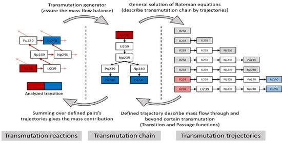
The graphical representation of the linear chain method is presented in
Figure 1. The linear chain method procedure can be presented in the following way. The transmutation chain structure, characterised with transition rate dependencies, is represented by a transformation map of decay and transmutation reactions. The structure is decomposed into a corresponding series of linear transformation chains and solved individually, assigning transition rates in the same way as in the decay problem. Finally, the solution of the general chain comprises the superposition of all linear chain solutions.
Unlike the Matrix Exponential Method, where there is one equation in the matrix form, the transformation equation is represented by a set of first-order differential equations, where each set represents one transmutation linear chain as a sequence of direct nuclide to nuclide transitions, starting from the first nuclide and ending at the last nuclide, like in the decay chain. The influence of neutrons invokes a more complex problem than in a simple radioactive decay case. The radioactive decay problem is connected only with sequential reactions leading to a stable isotope. Under irradiation, sequential reactions tend to form higher mass nuclides counteracted by the decay phenomena of the alpha, beta and other decays governing the transmutations of transuranic elements. Sequences of those nuclear reactions form transmutation chains, which are used for the description of the transmutation process. Under irradiation, every nuclide undergoes transformation. Therefore, nuclide stability, as in the decay problem, cannot be the criterion for chain termination, and therefore another criterion of mass balance has to be applied.
3.1. Transformation Equations for the Transmutation Chain
The transformation equation for the transmutation linear chain (Equation (9) and Equation (10)) is extended from those formed for the decay chain problem by numeration and branching consideration. The final solution for the transmutation trajectory takes into consideration a reduced chance for each transition, because it has an additional parameter of the branching factor, defined as the product of all transitions (Equation (13)).
where,
The solution of the last nuclide density in the chain is expressed as follows:
where,
It should be noted that in the case with no recycling, formula (12) can be used for every nuclide in the chain, but the densities at time t are not actual densities of considered nuclides but the contribution to the densities due to transformations only in this particular chain. For the introduced concept of transmutation trajectory, only the last in the chain nuclide density contributes to the overall density change, since in the trajectory building process the nuclides between the initial and the last one already occurred in one of earlier created trajectories as the last nuclide of the trajectory. Therefore, formula (12) will be used only for the last nuclide in the respective trajectory.
3.2. General Solution of Bateman Transformation Equations
So far, the solutions of equations with a different coefficient (Equation (13)) was discussed. The solution presented above would face undefined chains if the trajectory contained two or more equal lambda coefficients. This happens most often when some nuclide appears in the trajectory more than once, thus leading to the complication in the analytical solutions. Two ways of solving the problem are provided. The first method artificially shifts equal constants. If an appropriate small value of those shifts is introduced, it will produce accurate results for numerical calculation. However, in some cases characterised by a high neutron flux, the shift procedure can face a digital limitation. That is why the second exact general method has been derived. The general method expands the first method by finding the limit of shifts value when it approaches zero. The general solution allows for using equal constants and does not face a digital limitation. The final form is presented in Equations (14)–(16).
where,
and,
The branching factor has the same definition as previously (Equation (13)), but the analytical form is more complicated. In the general solution, it is usual to repeat the transmutation constants , each repeated mi times. In such a way, for a chain of nuclides that has a different transmutation constant, the sum is . If there is no repetition, the solution is equivalent to the solution from Equation (12). The remaining parameters are defined as follows: and is the Kronecker delta.
Here also the formula for density (14) will be used only for the last nuclide in the trajectory.
4. Transmutation Trajectory Analysis
Transmutation trajectory analysis is the process of breaking down the general transmutation chain into its elements—the transmutation trajectories, with their analytical characterisation, which allows us to reconstruct the general transmutation chain in a form of trajectory series under the control of the transmuted mass flow in the transmutation phase space. The transmutation trajectory is the elemental piece of the transmutation chain construct.
Every transmutation trajectory is defined by the path that leads from the initial nuclide to the final nuclide over which, for a given time, the mass transferred to the last nuclide is calculated (called transition) and beyond the last nuclide (called passage). The path is simply the series of sequential reactions that lead from the initial nuclide to the last nuclide of a particular trajectory.
Trajectory transition is essential for the calculation of the number density fraction that goes from the initial nuclide to the formed nuclide for a given time
t, in a sequence of reactions that follows the trajectory path. It is defined as:
where parameters
B and
are defined in Equation (13). Each transition ranges from 0 to 1 and describes the quantitative part of the transmuted nuclide. The respective sum of calculated transitions is used to calculate the nuclide mass for the calculated period.
The partial activity of a given nuclide considered in the chain is represented by the relation:
The defined activity concerns only the contribution from the
n-th nuclide concentration and disintegration along the considered trajectory. The disintegration rate for the considered period leads to the function
in Equation (19), which describes the sum of concentrations of nuclides formed as a result of the nuclide disintegration.
where,
The equivalent definition of the disintegration rate can be found as the previously mentioned sum of concentration daughters after being produced from the transition along the considered trajectory. It is possible to assume that the next nuclide is artificially stable, in order to obtain a less confusing definition Equation (21), although the computational cost is the same.
Finally, the trajectory passage is defined as the total removal rate of the considered trajectory or a fraction of the nuclide in a chain that passed beyond the nuclide and would be assigned to the following nuclides in the chain for the considered period.
Transition and passage are absolute parameters for the examination of the integrity of the transformation system and mass balance. They are used in a numerical algorithm that generates the series for trajectories and resulting nuclide transformations representing the general transmutation chain. It should be noted that there is no single algorithm which can be realised, and code developers may refrain from disclosing the detailed solutions. Particular solutions can be effective of not, booth in calculation speed and calculations errors.
5. Numerical Generation of Transmutation Trajectories
The TTA was developed for the numerical control of breaking down the general transmutation chain into a series of linear chains. This is actually dome by the construction of the transmutation trajectory series independently for every initiating nuclide which appears in the mass vector at a given time point. Functions
T(
t) and
P(
t) allow for the formation of a transmutation chain that reflects the formation process of transformation in reality. The generator controls the mass balance in order to properly form the chain series. The procedure starts from the outermost iteration loop finding each parent nuclide (root) with non-zero initial density. It is an ancestor for other arising nuclides at the end of a computational step. Each parent nuclide builds its own set of linear chains, called a family [
19]. The assumption is that the densities of all other nuclides beside the parent equal zero at time zero. The first trajectory generation contains one possible trajectory (there is only disintegration rate, Equation (9)). The nuclide remains for the next step, but is represented physically by the survival of the initial nuclides which avoided any nuclear reaction. Equation (23) and Equation (24) express the first trajectory generation. The first suffix is the current trajectory number, while the second suffix is its parent trajectory number.
Subsequent trajectory generations are formed by finding all possible nuclide paths using all possible nuclear reactions from the current trajectory. Next, the calculation of the functions
T(
t) and
P(
t) is performed for those second trajectory generations. The trajectories of the second generation are considered as daughter trajectories of the first generation. After the extension of all possible reaction channels of trajectory
k to daughter trajectories from
l to
f in a way that
, the next generation of daughter trajectories belongs to the newly explored transmutation path and fulfils the balance relation:
where the first suffix is the current trajectory number, while the second suffix is its parent trajectory number. The process of trajectory extension is recursively repeated for each previously defined trajectory. During this process, chains are extended by reaching the subsequent trajectory generation. Each trajectory length is defined as the number of transformations in trajectories increased by one process, which is the avoidance of disintegration by the root nuclide. During this process, the passage value decreases from transformation to transformation, by the value of the trajectory transition
T(
t)
, which is different for different transformations but independently from the time used for the termination of the chain extension, thus avoiding an infinite growth of the trajectory number. The application of the number density, and therefore the mass conservation, is performed for every trajectory extension. It is realised in the following way. The residual passage
R(
t) is the sum of the trajectory passages which have not been extended in the considered family, where the generated series contains
m completely extended trajectories. The definition Equation (26) uses
X as a set of parent trajectory indexes.
The total transmutation transition is defined as:
Finally, number density, and therefore mass conservation, is expressed as the sum of the total transmutation transition and the residual passage,
The physical interpretation of the above relations is as follows. The residual passage represents the fraction of concentrations that was not assigned to any nuclide, whereas the transmutation transition corresponds to the assigned fraction. With each trajectory extension, the residual passage Rm(t) always diminishes due to the decreasing passage (Equation (25)). Thereby, the passage parameter is suitable for the truncation of the trajectory series. The simplest, but not the best solution is the application of a single threshold parameter ε for all instances of trajectory extension. It determines the minimal value of the trajectory passage which undergoes extension. This, however, can result in the elimination of nuclide formation of very low transmutation transitions, but maybe of interest. The solution for this is the introduction of the additional condition of accepting the extensions when the nuclide to which the transformation goes was not yet built from other roots and the passage is below the constrained relative precision of calculated density.
Any procedure of trajectory extension process based on a fixed threshold will preserve the generator from an infinite extension of trajectories and introduce a straightforward numerical parameter for the control. After the formation of all trajectories, a general transformation map of decay and transmutation reactions is represented by a linear chain system. In a trajectory set defined in such a way, the contribution to any particular nuclide, e.g.,
k-th is obtained by the summation of the respective transitions.
where
ix(
m) is the index of the last nuclide in the
m-th trajectory.
Although someone could think that TTA creates infinite series of transitions, in reality the linear chain length (or number of involved sequential reactions) is limited by the nuclide mass or the number of atoms that are left to be assigned to a particular nuclide. In that sense, the transition rates below a single atom will not even be observable in reality. In practice, any physical transmutation system can be described by a limited number of linear chains. Moreover, the uncertainties of calculated densities are dominated by the reaction rates’ evaluation uncertainty as well as by the errors associated to the deviation of real transmutation probability rates form the transmutation constant; therefore, a very low threshold for chain extensions loses its purpose.
The basis of the solution of transformation equations using TTA is the build-up of the transmutation chain in the form of a series of transmutation trajectories that are generated, based on already generated trajectories, by their extension, while controlling the mass flow and depending on the actual reaction rates concerning the reaction that leads to trajectory extension. The construction of the transmutation trajectory series starts from the first trajectory, defined as a survival of the initial nuclide over step time. The trajectory transition equals the fraction of initial mass that was left after step time, while the trajectory passage is the faction of initial mass that underwent transformation. The first trajectory mass balance is obvious, since the sum of the passage and the transition equals one. The next trajectory is an extension of the first trajectory by any possible reaction from the last nuclide of the parent trajectory. For the first trajectory, as a parent, the last nuclide is the same as the first one. If few different reactions are possible, a trajectory tree will be formed branch by branch, but sequentially. The passage value from the parent trajectory is divided into branches proportionally to the branching ratios. For each newly formed trajectory the transition and passage are calculated according to TTA formulas (based on Bateman solutions). The passage value in every extension decreases and represents the amount of mass that is still afloat, while the trajectory transitions represent the contribution to the final mass of the nuclide standing at the end of the trajectory. The mass afloat for the entire system is the sum of all the trajectories not yet extended. With every trajectory extension, the sum of mass assigned to any nuclide increases while the sum of the afloat mass decreases. Each possible trajectory extension is analysed if it can possibly contribute to the mass of any nuclide above the defined threshold. Two possibilities here exist that can be treated differently. The first one is the transition to a nuclide which already has an assigned mass transferred by other trajectory. For such a case, one can apply the defined level of calculation’s relative precision of density—for example, 10−5. In this case the threshold for the passage value (the cutoff parameter) can be set at the designed relative precision multiplied by the already assigned mass fraction—for example, 10−2, and divided by the predicted number of trajectories of the first and the last trajectory nuclides. Typically, the number 100 can be safely assumed. In this case the passage threshold of 10−9 can be safely assumed. The second possibility occurs when the reaction leads to a nuclide to which no mass has been assigned. In this case, the truncation threshold should be set to the desired level, but not less than the transition rate of a single atom. This is an inverse of the number of initial nuclides at the beginning of the step. More practical for a typical reactor analysis is to assume the trajectory cutoff parameter at the level of 10−10, which typically guarantees that the unassigned mass will not exceed 10−6 g. More rigid conditions can increase the calculation time, but they can be applied conditionally, for the required nuclides can also be set by the user. It is worth mentioning that the calculation time needed for TTA modules is substantially lower, by one or two orders of magnitude, than the time required for neutron transport simulation in Monte Carlo transport simulations, which involves transmutation probability rates calculations.
In the various approaches to the solution of a large transmutation system, there is a dedicated treatment of short-lived nuclides. In practice, for a typical case, the step time can be used for the discrimination of a short-lived nuclide treatment for reducing the calculation print-outs and the calculation time. This treatment assumes an instant decay of short-lived nuclides which does not noticeably affect the actual transition to longer-lived or stable nuclides. This treatment never eliminates the formation of any nuclides, even those that are short-lived. Their densities can be calculated using the densities of their precursors. The savings that are being made are more significant, due to the reduction of the time required for reaction rate evaluations, rather than the savings obtained with the Bateman solutions. Finally, in the defined set of chains, the total transition from one nuclide to another is a sum of all the defined transition chains, beginning with the considered nuclide and ending with the target one.
The passage for short trajectories can be high, but it decreases in daughter trajectories. New trajectories (daughter trajectories) are generated by extending the already formed trajectories if their passage is above the defined threshold. This sort of processing allows us to consider the meaningful transformation chains and exclude those with low (actually with extreme low) contribution to the already calculated mass transfer. Control over chain formation is a crucial attribute for the extension of the transformation chains that characterise each computational step. The offered direct solution method uses a versatile transformation calculation system that potentially involves thousands of nuclides, which can even create millions of different transmutation transitions if the cutoff threshold is set very low.
Algorithms based on the TTA method can be improved in terms of efficiency by several means, like: execution of involved sums in order to generate the smallest digital error; identification and utilisation of recursive formulas; identification and utilisation chain characteristics obtained in past steps or neighbouring cells; testing various cutoff definitions depending on the considered case.
Since TTA algorithms can have many variants, it is recommended to present a detailed description (step by step) of the applied procedures.
6. Linear Chain Method Sample Problem
The small transformation map of decay and transmutation reactions during time
t, which is shown in
Figure 2, is considered. The rates of transmutation interactions are characterised by the total removal rate. The branching coefficients (Equation (11)) show the direction of a given reaction, i.e., the fraction of the transmutation transition from one nuclide to another. In the presented example, the following assumptions were made:
- -
at the beginning of calculation, only 238U is present. All other nuclide densities equal zero;
- -
the neutron flux is constant and normalised to ;
- -
reactions such as the production of fission nuclides, (n,2n), (n,α) and some transmutations, are neglected for the range of neutron energies present in power reactors.
The transformation map consists of six nuclides after the irradiation period. The general solution is described by six first-order differential equations. The linear form of the problem can be extracted from the general chain using the TTA method. Since at the beginning only
238U is present, TTA forms six transmutation trajectories. Only the first three trajectories are shown for the sake of presentation simplicity. The first trajectory contains only the ancestor nuclide (
Figure 3). Physically, it represents the non-transmuted nuclide mass. The passage represents the contribution of the mass that goes beyond the current trajectory. It is clearly visible that
, where
. If the passage is less than the cutoff parameter, then the procedure ends with a simple trajectory, where the passage is assigned to the residual passage. Such a situation would happen with the
238U reaction rate, if the considered time was very short.
When the passage of the first trajectory is higher than the cutoff parameter, a second trajectory is formed (
Figure 4). The second trajectory describes the contribution from the ancestor nuclide of
238U to the next of its direct descendant nuclides, in this case
239U. In other words, the second trajectory describes the transformation
238U→
239U. This trajectory is described by two transformation equations. The transition value is calculated from Equation (22). Mass balance is preserved by the relation
where residual passage is the sum of the second trajectory passages and the non-extended passage from the first trajectory,
. This relation shows that the trajectory extension process consecutively decreases the residual passage.
The third trajectory is extended from
239U (
Figure 5). It is built from three nuclides:
238U→
239U→
239Np, and it is described by the trajectory
. The procedure is analogous. The transformation equations are formed and solved by their linear solution, obtained using the TTA method. The mass balance is preserved by the relation:
With every extension of trajectory, we need to calculate only the transition and passage. The density of added nuclide—N3 will result from T3, while N1 and N2 were already calculated in the first and second trajectory, respectively.
After following the extension of the remaining trajectories, the final set, which describes the transition from the ancestor to its descendants, is obtained. This process is presented in
Figure 6. In the case where not only
238U is present at the beginning of the cycle, the outermost loop performs the trajectory extension for each ancestor nuclide of nonzero concentration. Each set of chains obtained in such a way is called a family [
19], indexed after the ancestor.
The last example (
Figure 7) presents the solution of a cyclic chain. In the standard solution, identical coefficients would lead to an undefined relation. However, it has been shown that the general form of the solution can be found using Equation (14). This example considers the trajectory of
238U→
239U→
238U, which contains two identical removal rates for
238U.
Here the density of added nuclide—N3 will be added to the final destiny of 238U, as calculated in the first trajectory N1, since it also represents 238U.
7. Method and Numerical Tool Developments and Comparisons
The evolution of the nuclear fuel inventory during irradiation is defined by changing nuclide concentrations, which influences the transition probability time rates. Therefore, neutron transport calculation must be performed for an efficient number of steps in the considered irradiation time.
The appropriate length of calculation periods is used to estimate average transition rates, which allows us to use a solution of the transformation problem coupled with neutron transport calculations. The solution presents nuclide composition at the end of the step, which is then used as the composition at the beginning of the new step, in a repeated procedure in a sequential manner. The final results of the simulation contain nuclide concentrations and other parameters, like, e.g., the effective neutron multiplication factor or power profiles, over time, until the destination time is reached.
The transmutation rates are obtained directly through a Monte Carlo process or indirectly as a product of reaction cross-sections and neutron flux in a more or less detailed geometry division of the irradiation system. Neutron transport calculation is used for the solution of the neutron steady-state problem, depending on the problem in stationary or eigen state. Depending on the problem in hand, the neutron flux and reaction rates are normalised to the assumed integral parameter, which can be a total system power (typically for a critical system), neutron source strength or ion beam current (in the case of subcritical neutron systems or ADS). These reaction rates are used to calculate transformation probability time rates, which became Bateman equation coefficients.
In this work, one of the latest version of the MCB5 code implemented on supercomputers of the Academic Computer Centre CYFRONET AGH was used for the computation time presentations. The practical issues related to the implementation and automation of the MCB code using Message Passing Interface at high performance computers are available in an associated paper [
20]. In the implementation, the benchmarking and validation process were carried out. The isotopic concentrations obtained using the TTA implemented in MCB were compared with other numerical tools (FISPACT and SWAT) within benchmarking studies [
21]. The following validation study was performed using data obtained from the destructive assay of fuel samples irradiated at the Japanese Ohi-2 nuclear power plant [
22]. In addition, the dependence of the TTA burnup calculations from the time step model was investigated in dedicated studies [
23].
Computation Time
Table 1 shows the comparison between computation times of Monte Carlo neutron transport (
TTr) and TTA burnup (
TBr) calculations for three benchmarks, i.e.: PWR reactor, HTR reactor and subcritical Th assembly with a Cf neutron source. The computation times cannot be directly compared in each case because of the different implementations of the numerical models due to various complexities of: geometry, material composition, number of time steps, number of neutron histories and cycles. However, the
TBr and
TTr for each case can be compared. The
TBr corresponds to the time between the end of the neutron transport calculations for the
nth the cycle and the beginning of the neutron transport calculations for the (
n+1)th cycle in the case of the eigenvalue (
Keff) calculations. In the case of the source calculations,
TBr is the time elapsed between the calculations of a given number of neutron histories for the two following time steps. In both cases, the TTA burnup calculations are performed between the two following neutron transport calculations. The
TBr contains all operations necessary for the calculations of the new isotopic composition using TTA as well as the time necessary for all numerical operations for the storage of newly created data. The
TTr corresponds to the Monte Carlo neutron transport calculations for given cycles (eigenvalue calculations) and histories (source calculations). In the analysis, the
TTr and
TBr for the time steps at the beginning of calculations (BOC) and at the end of calculations (EOC) are considered. The calculations were performed using 24 Intel Xeon E5-2680v3 CPUs (2.5 GHz) by means of the MPI interface. The cutoff value of 10
−10 was assumed. In all cases,
TBr is much lower than
TTr, which shows that the TTA burnup modelling is much faster that the Monte Carlo neutron transport modelling. In first two cases, the times for the initial time steps are lower than for the final time steps, which is caused by the formation of the new isotopes in the burnup process, the increase of numerical model complexity and thus the computation times. In the last case, the times at BOC and EOC are the same due to the limited formation of new isotopes by the lack of fissionable material in the system.
The main advantage of the linear chain method is that linear chains represent series of physically occurring nuclide transitions that preserve the entire quantitative information about the transformation process. This might not be needed if one is interested only in density evolution in simple cases. However, if one is also interested in the calculation results confirmation, an alternative method is needed. If one needs a calculation error assessment, then the calculation error associated with intensive algebraic calculations in the matrix approach must be included. Contrary to the matrix approach, there is no numerical issue to calculate transmutation transitions in the TTA approach for any possible physical system. The matrix methods are always based on numerical approximations, which for a simplified and well defined system can be demonstrated as very effective and fast, but generally they are case-dependent, and it cannot be guaranteed that for more complex systems the uncertainties of the results are at the same level as in the tested case. The computation time used by the TTA depends on the complexity of the defined numerical problem as well as on the available hardware. With the low value of the cutoff parameter or long period length due to the increase in the produced number of trajectories, TTA would require more computation time than the methods using the exponential matrix solution [
24], but for cases of radioactive decay TTA can be faster and more accurate. For the transmutation system, as it was shown above, in order to reduce calculation errors, must be devoted most of the time to Monte Carlo transport simulations and apply time steps that are not too long, while savings on transmutation calculations are actually negligible. Recently, several developments concerning TTA formulas have been reported, modifying algorithms using backtracking [
25] or using recursive formulas [
26,
27]. Moreover, an alternative cutoff check, which utilises the time-averaged number densities, is claimed to reduce the calculation time by a small factor.
8. Summary and Discussion
In the paper, the derivation of the linear chain method for solving the Bateman transformation equation was shown. The general solution for a linear chain together with the trajectory generator provides a numerical tool for solving transformation equations, which represent the physical nuclide-to-nuclide mass flow. The advantage of the linear chain method is that the result represents the exact series of physically occurring nuclide transitions, which preserves the entire quantitative information about the transformation process. This feature helps determine if the calculation process was corrupted, whether due to introduced program bugs or data corruption. The calculation results obtained using the TTA approach were in every reported calculations the most accurate; therefore, TTA is used as a tool for verifications of numerous burnup codes that apply matrix methods.
After all, the solution of the burnup problem performed using the TTA approach delivers the nuclide compositions at the end of the computational period in the same way as the matrix exponential method. The TTA method has been initially implemented in MCB [
13,
20] over twenty years ago, while recently, with a significantly growing interest in developing new codes, several realisations include TTA, including Serpent [
28] and the most recent ones, with modified algorithms based on recursive formulas: DEPTH [
29], OMCB [
30], IMPC [
31] and MODEC [
32].
Nowadays, an increased interest in the development and implementation of numerical tools for sensitivity and uncertainty analysis is observed [
33,
34]. Many new uncertainty analyses focus on the calculation of uncertainties associated with the computed nuclide concentrations. The final uncertainties have to take into account the uncertainty in the decay and transmutation constants, space-energy integrated neutron flux and evaluated cross-section data. In addition, in burnup calculations the uncertainties propagate in burnup functions, which makes the task more complex. The TTA method is dedicated to coupling with Monte Carlo transport codes, and it keeps the philosophy of the Monte Carlo approach, which is to represent physical phenomena as close to reality as possible. This is why the preservation of the information about the transmutation structure is important. Yet Monte Carlo methods are still under development, for example concerning error propagation and sensitivity analysis. For that purpose, TTA offers the possibility of calculating sensitivity coefficients in a direct simulation process. The information embedded in the set of trajectories is a basis for a detailed transmutation assessment of individual transmutation chains, which cannot be provided by the exponential matrix method. The development and utilisation of the trajectory period folding methodology [
35] could help in quantifying the impact of a set of input parameters on the integral output parameter. The trajectory period folding approach can be expanded with the uncertainty propagation and used in validation studies in order to assess the accuracy and reliability of calculations, which is foreseen for future work.


