
High Performance Electric Vehicle Powertrain Modeling, Simulation and Validation


Abstract
1. Introduction
2. Equation-Based Modeling Summary
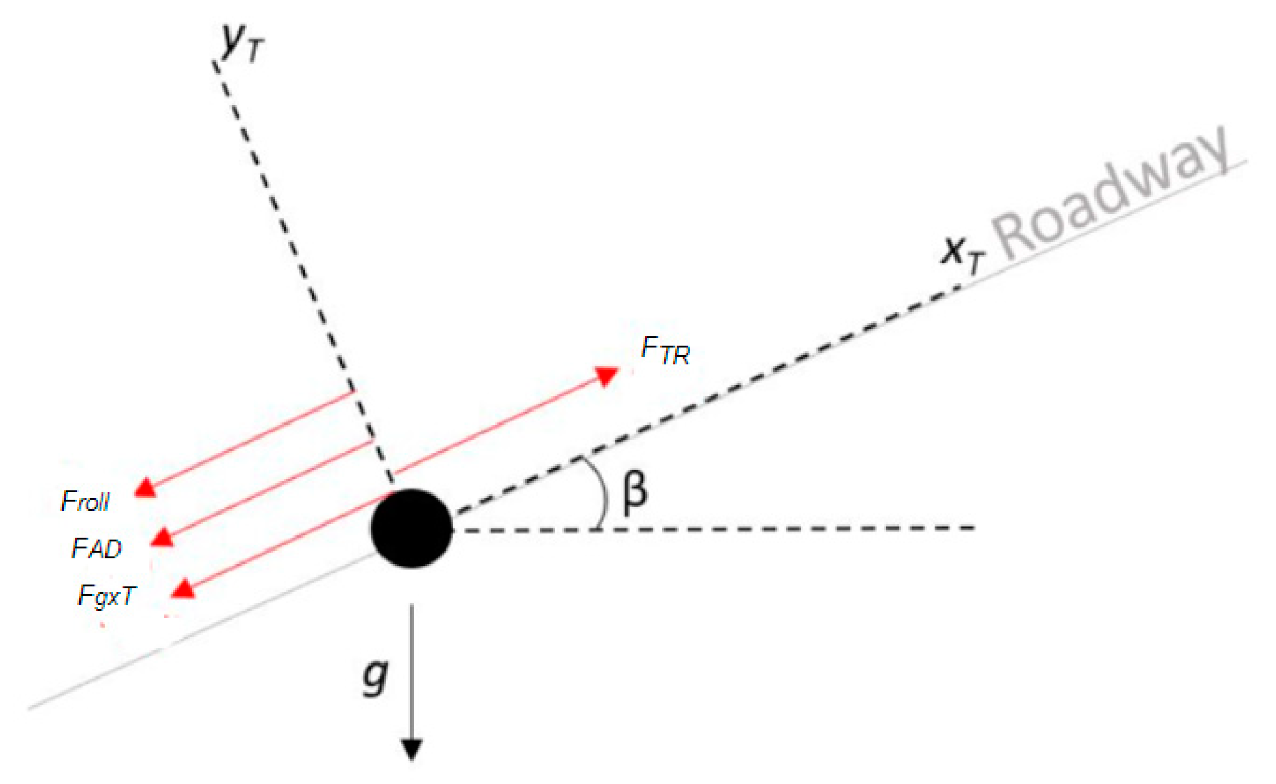
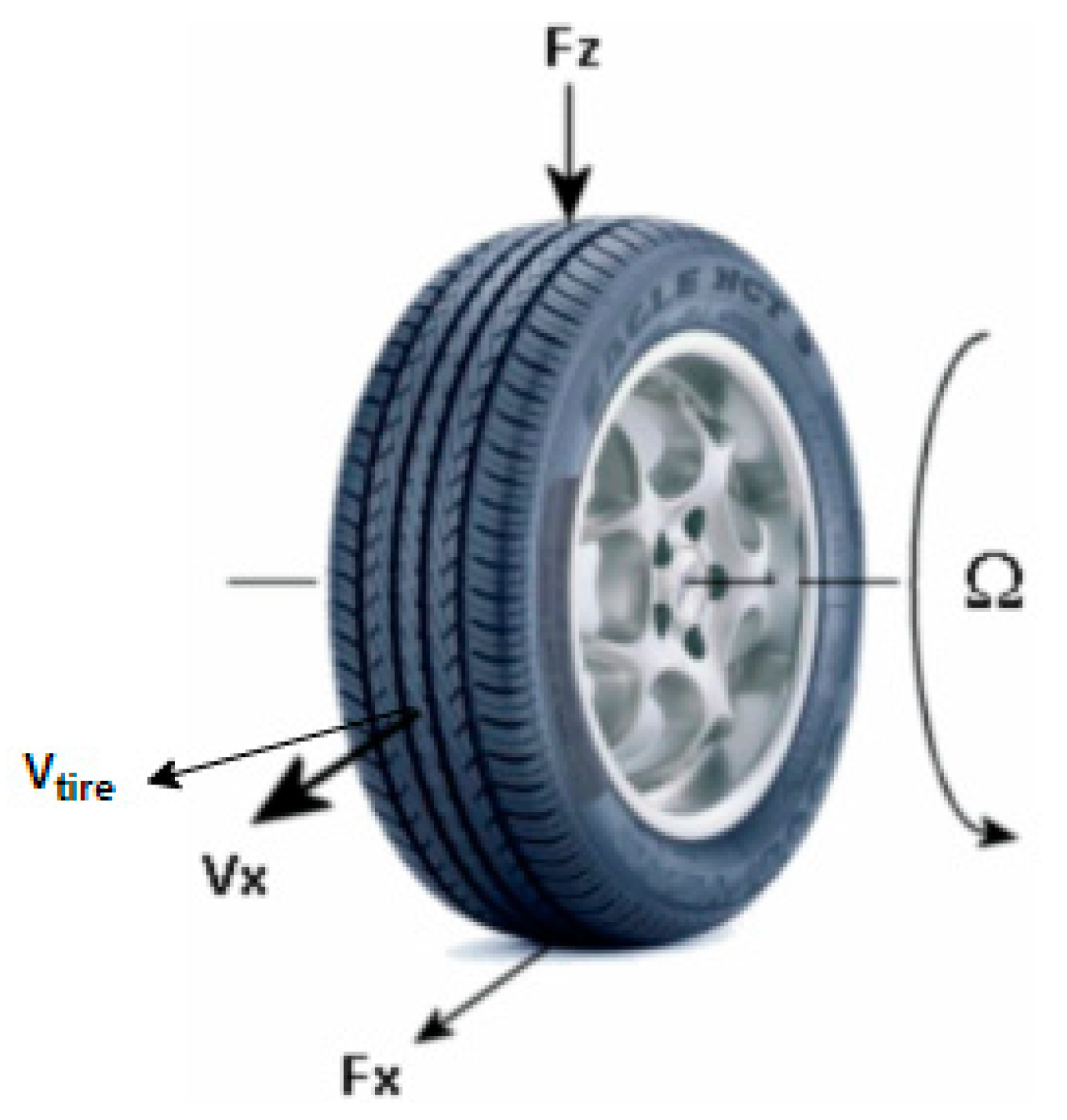
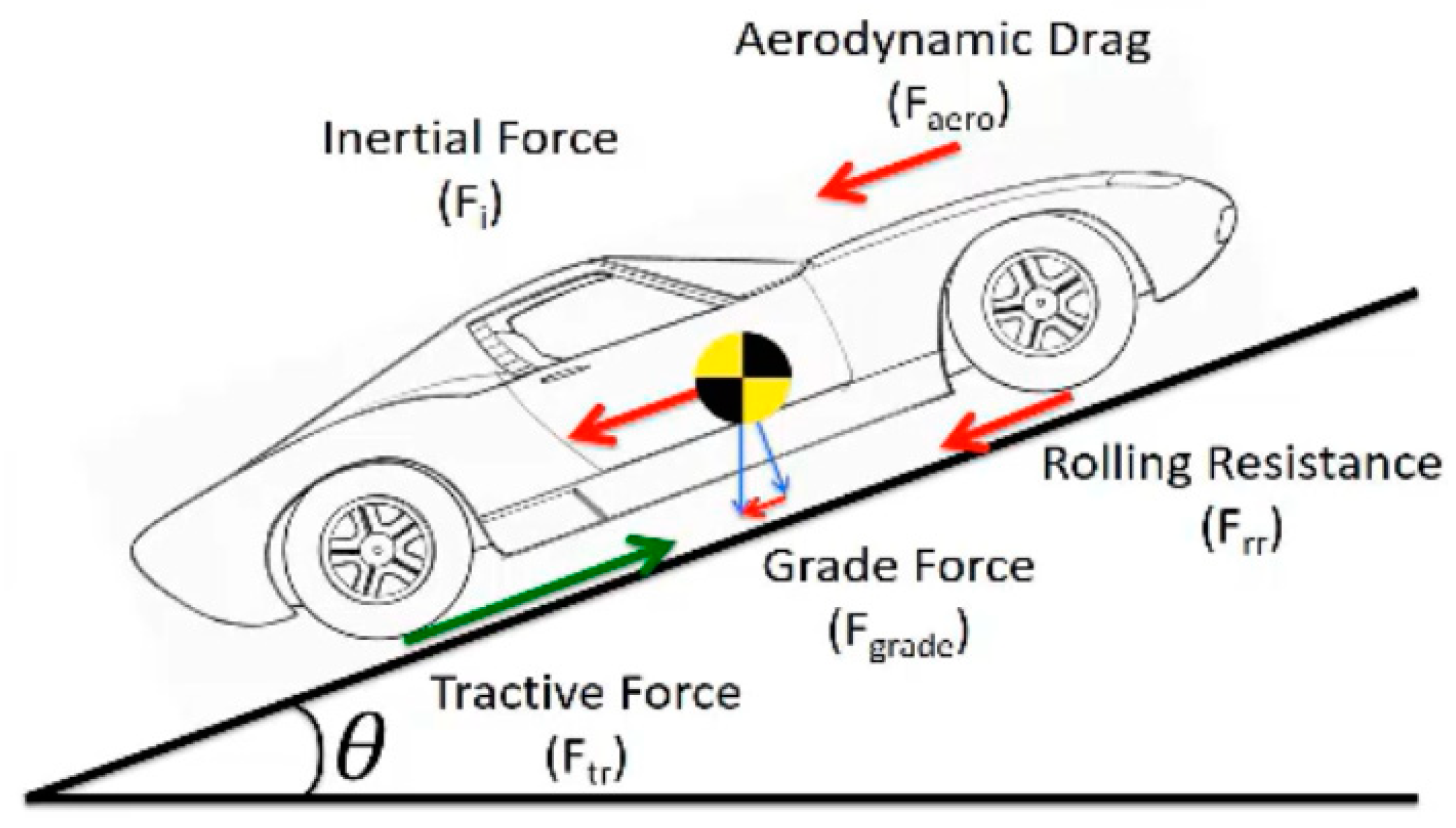
2.1. Dynamics of Vehicle Motion
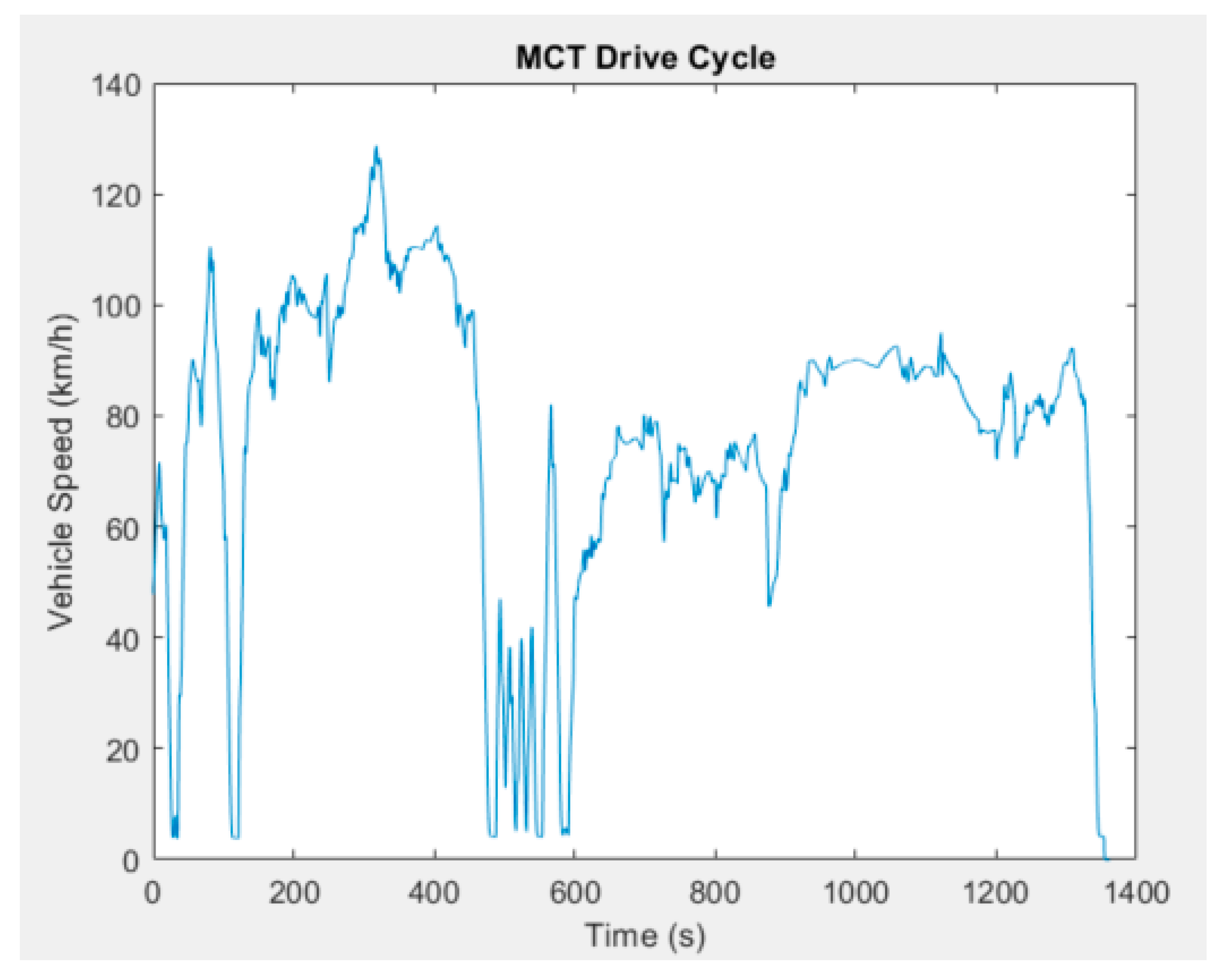
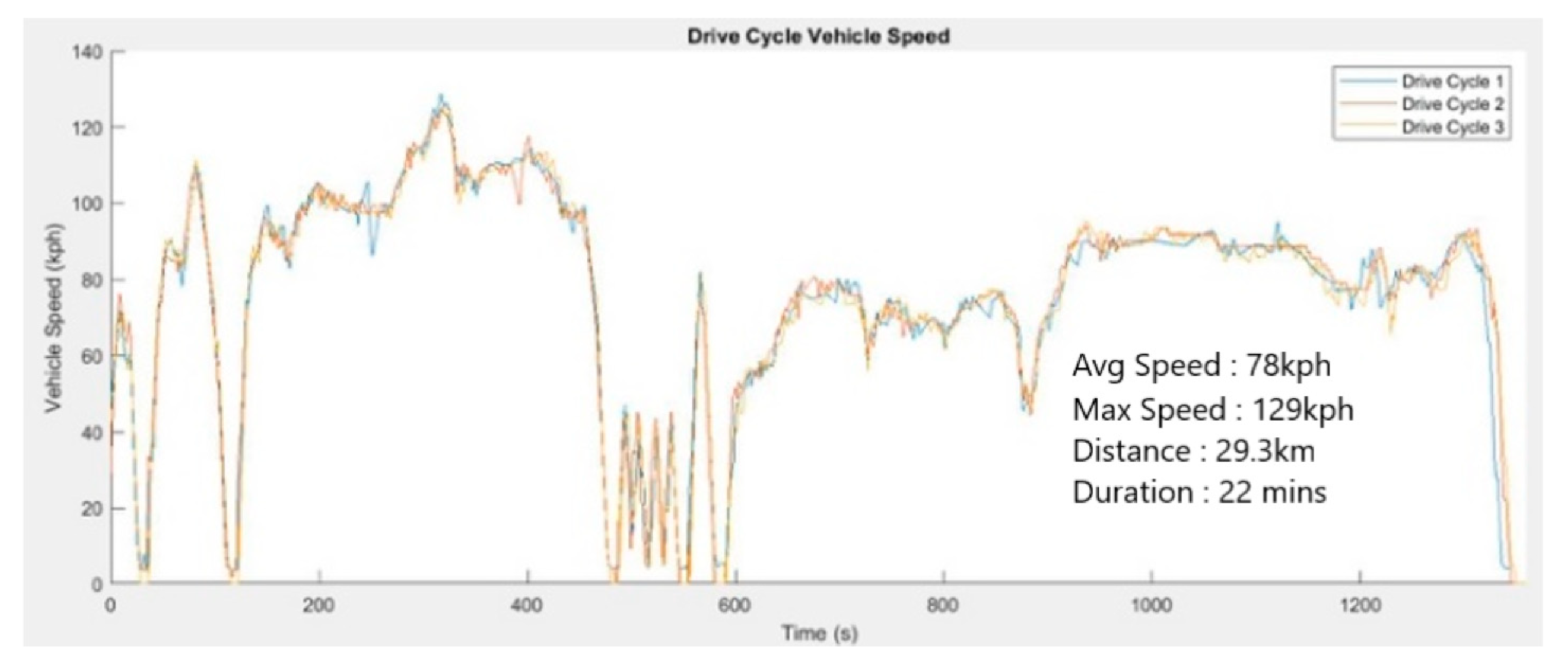
2.2. Drive Cycles for Modeling and Testing
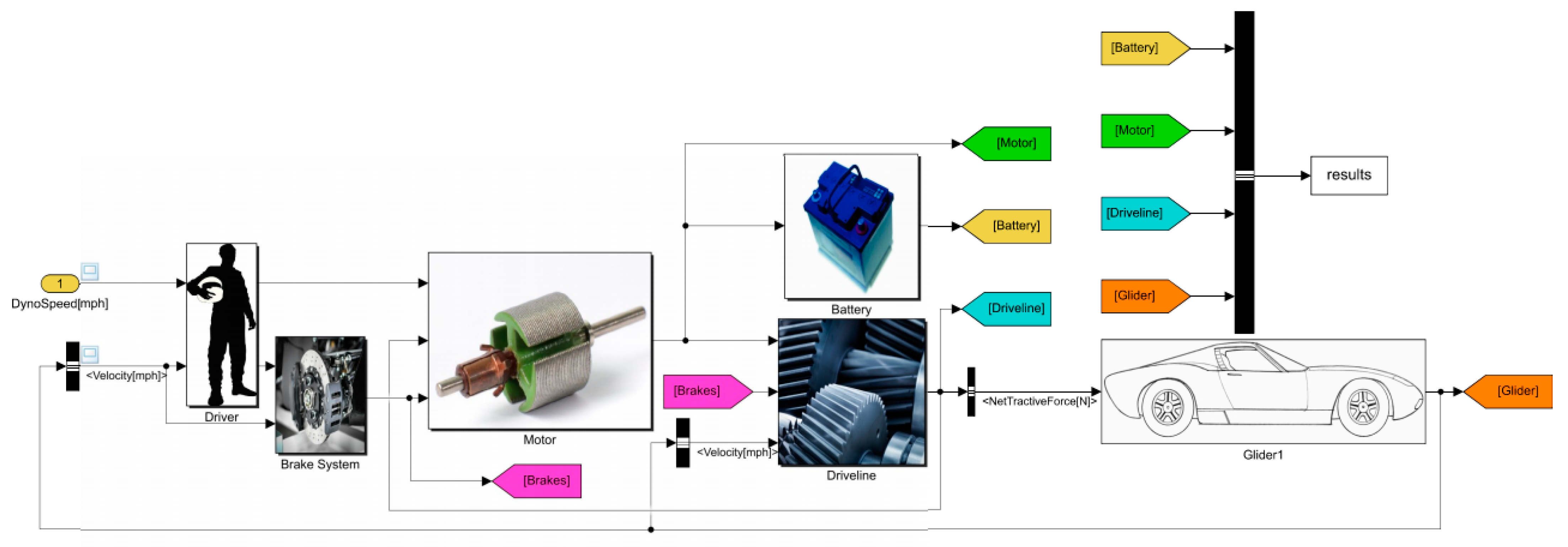
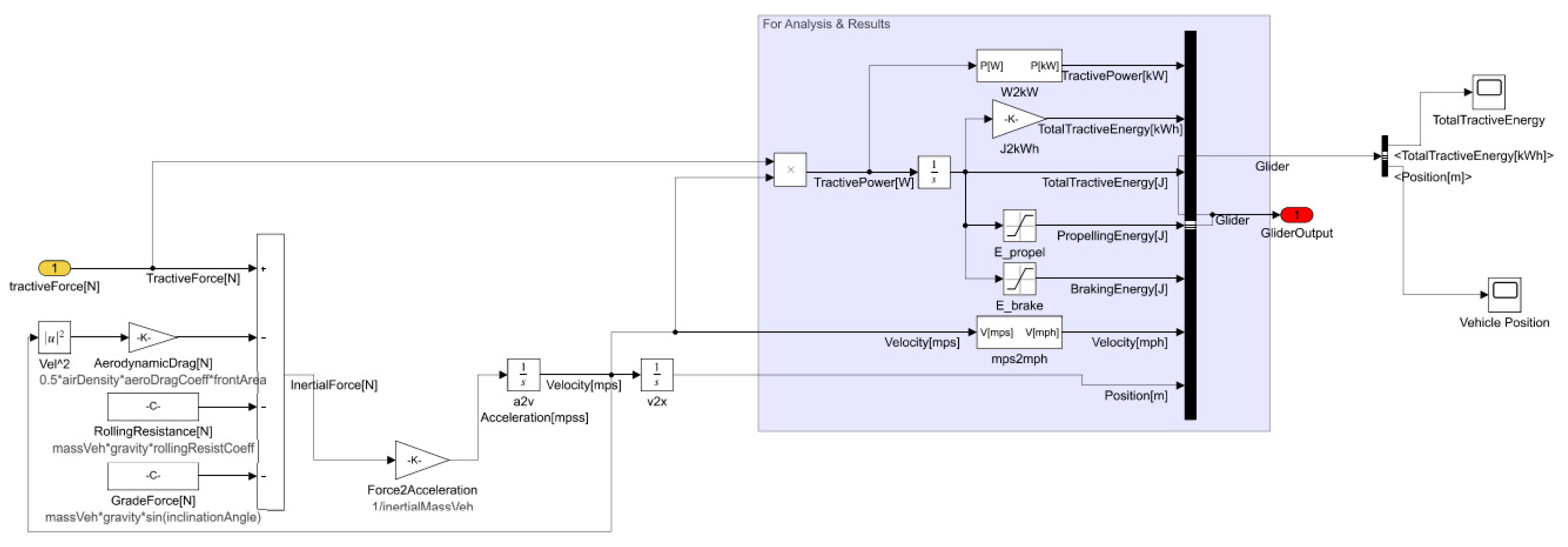
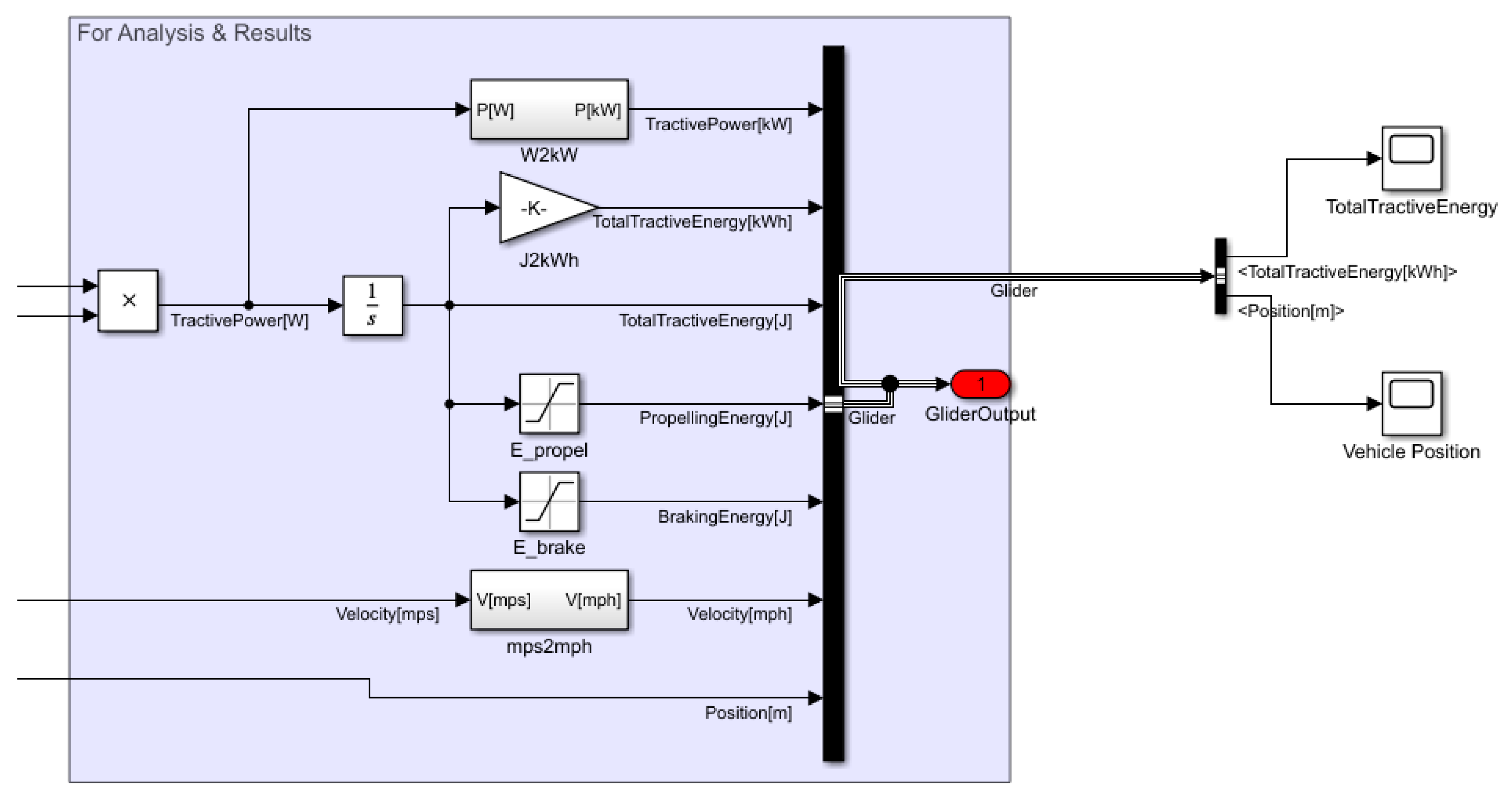
2.3. EV Powertrain Modeling and Simulation
2.4. Glider Model
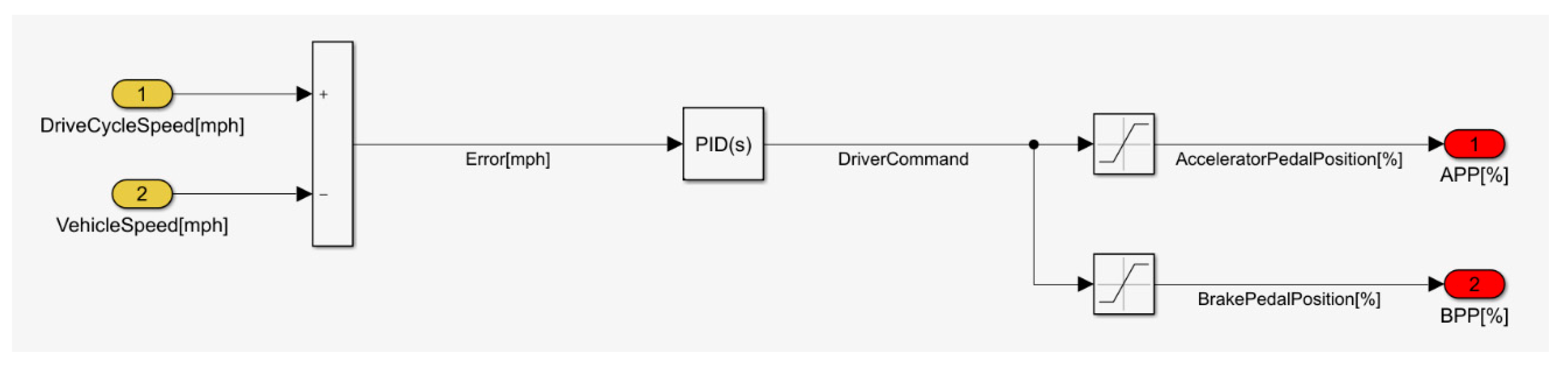
2.5. Driver Model
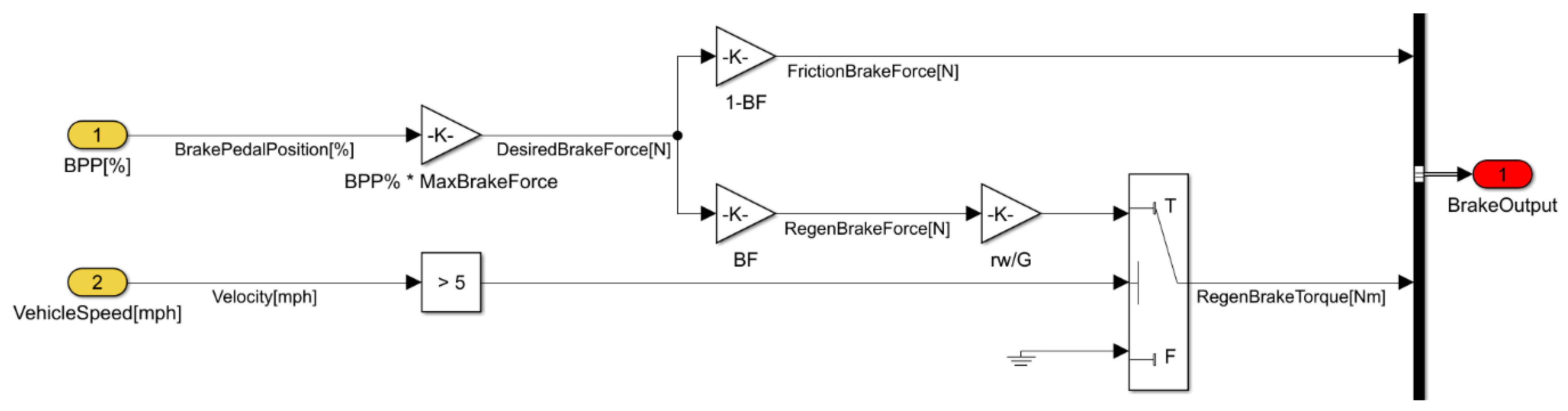
2.6. Brake System
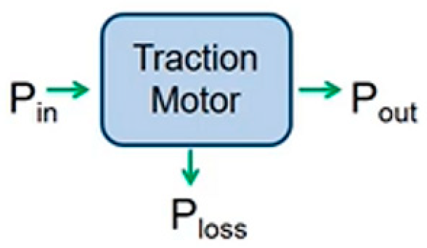
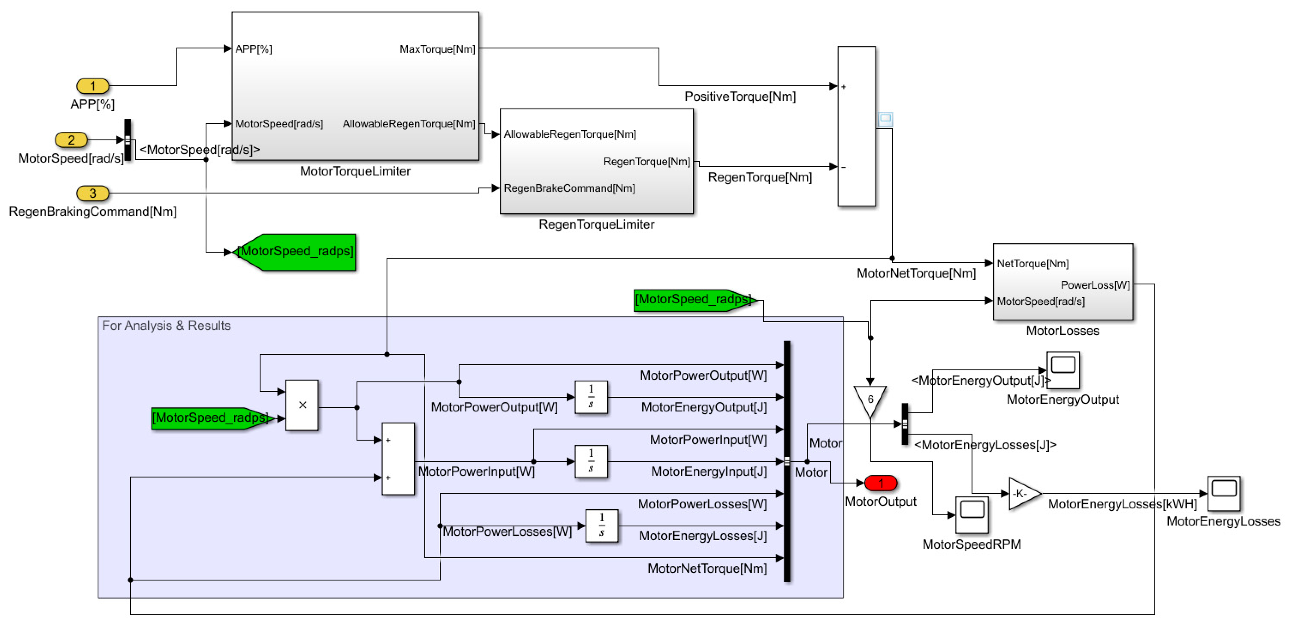
2.7. Motor Model
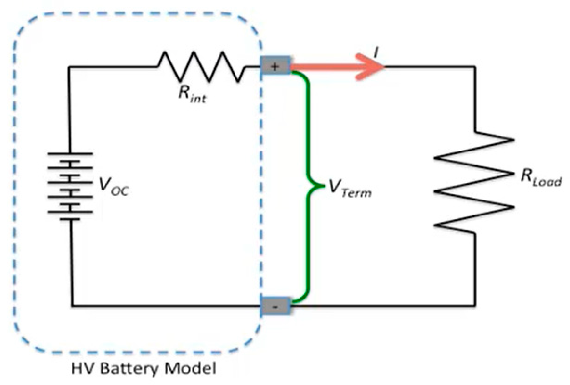
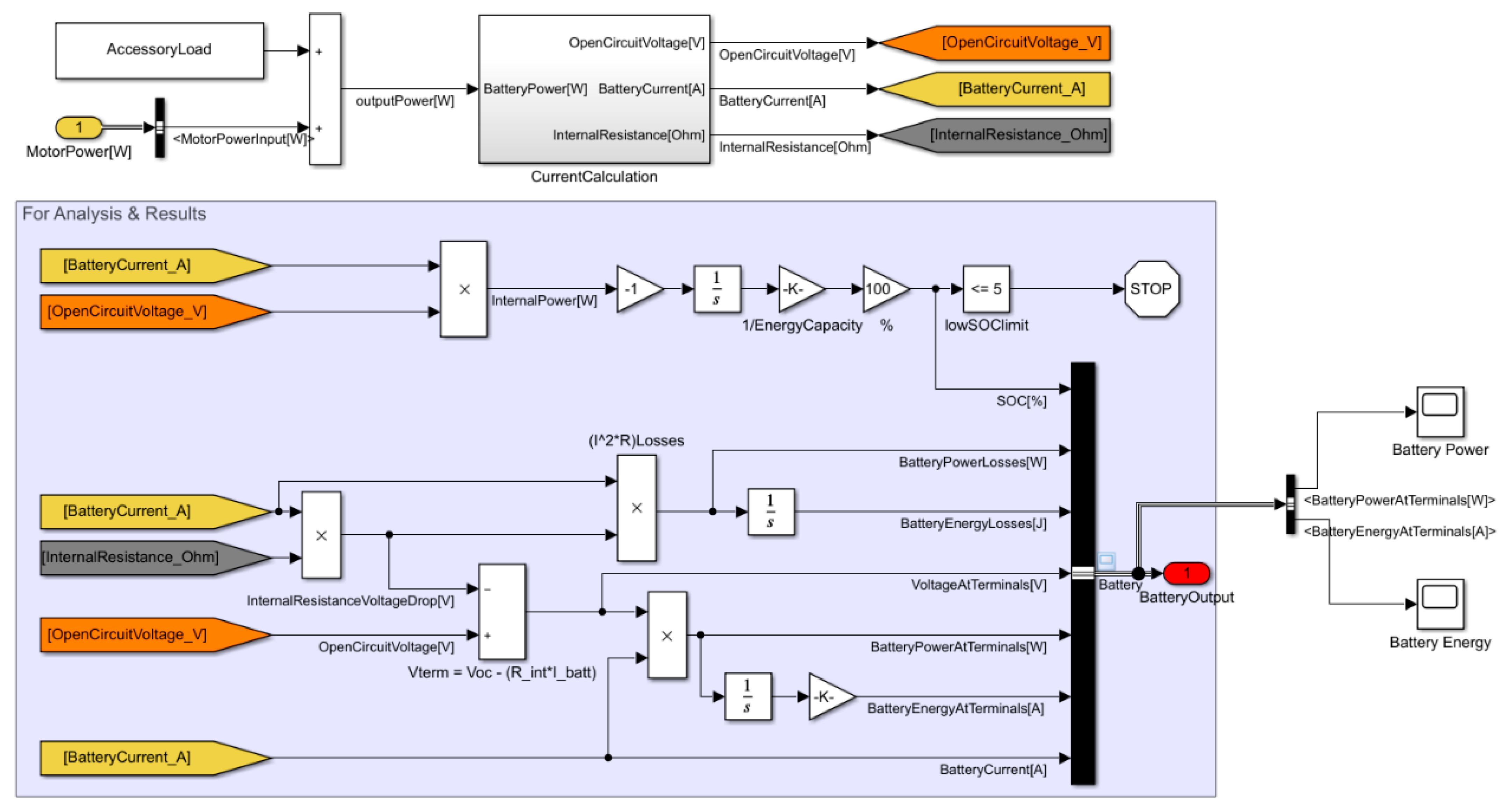
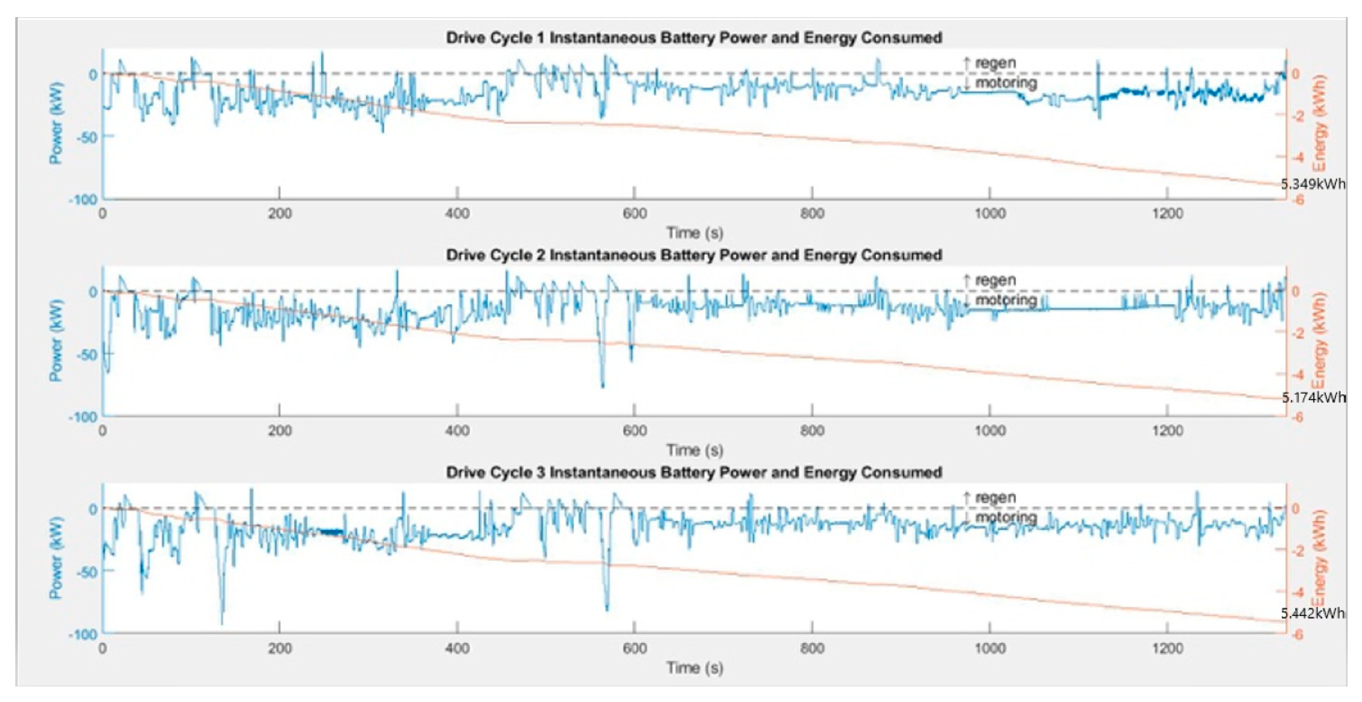
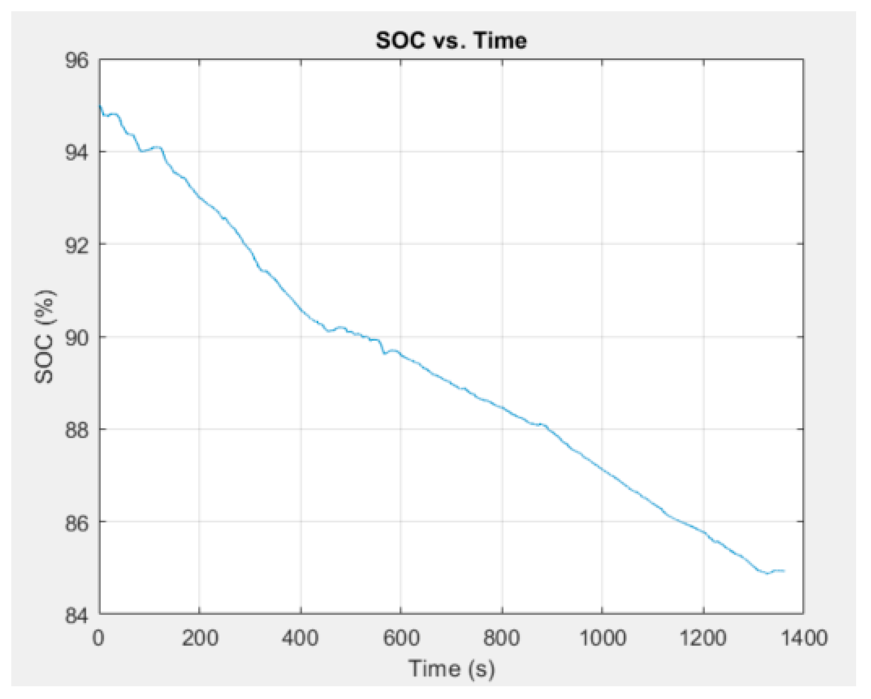
2.8. Battery Model
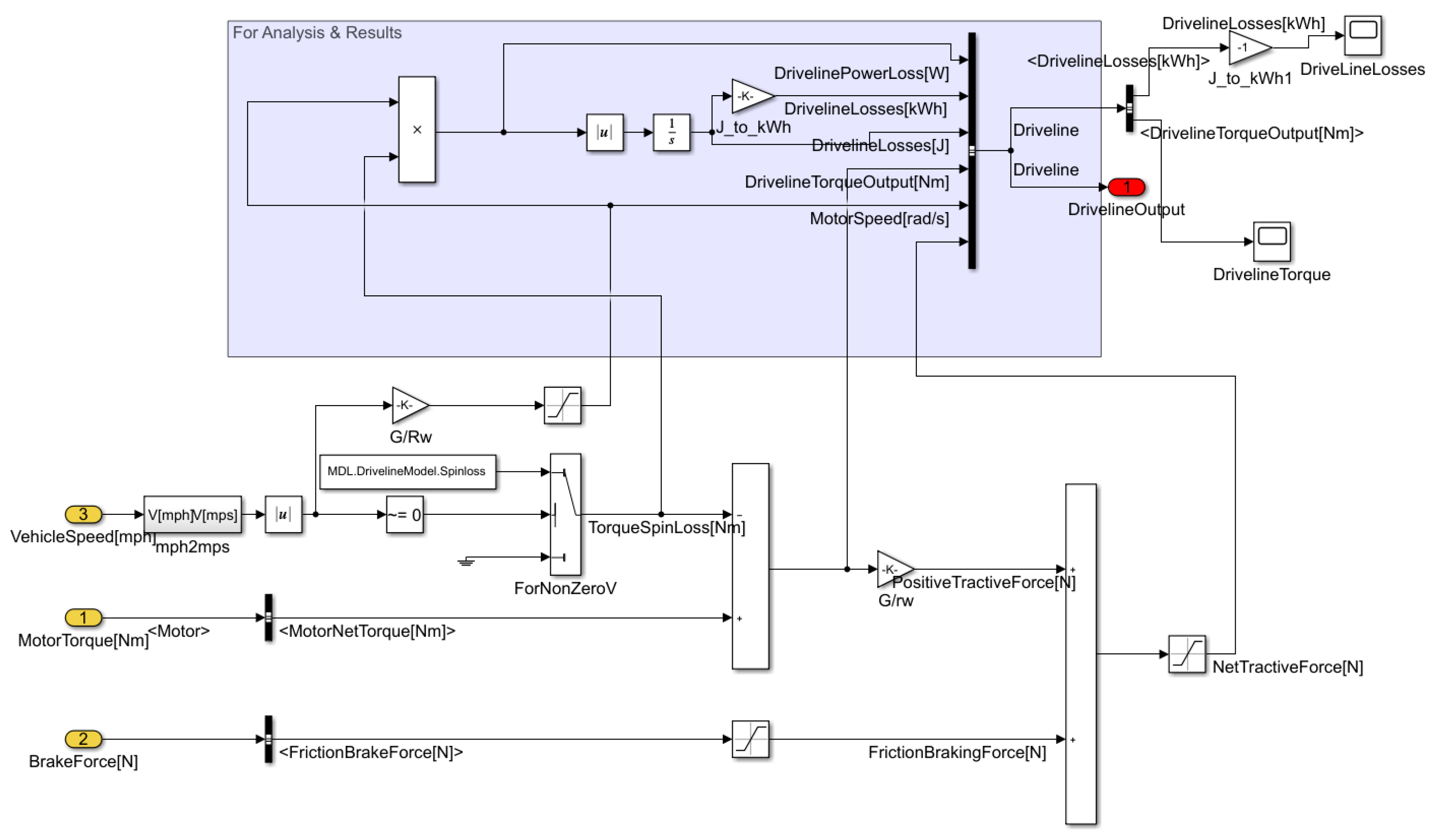
2.9. Driveline Model
3. EV Chassis Dynamometer Testing
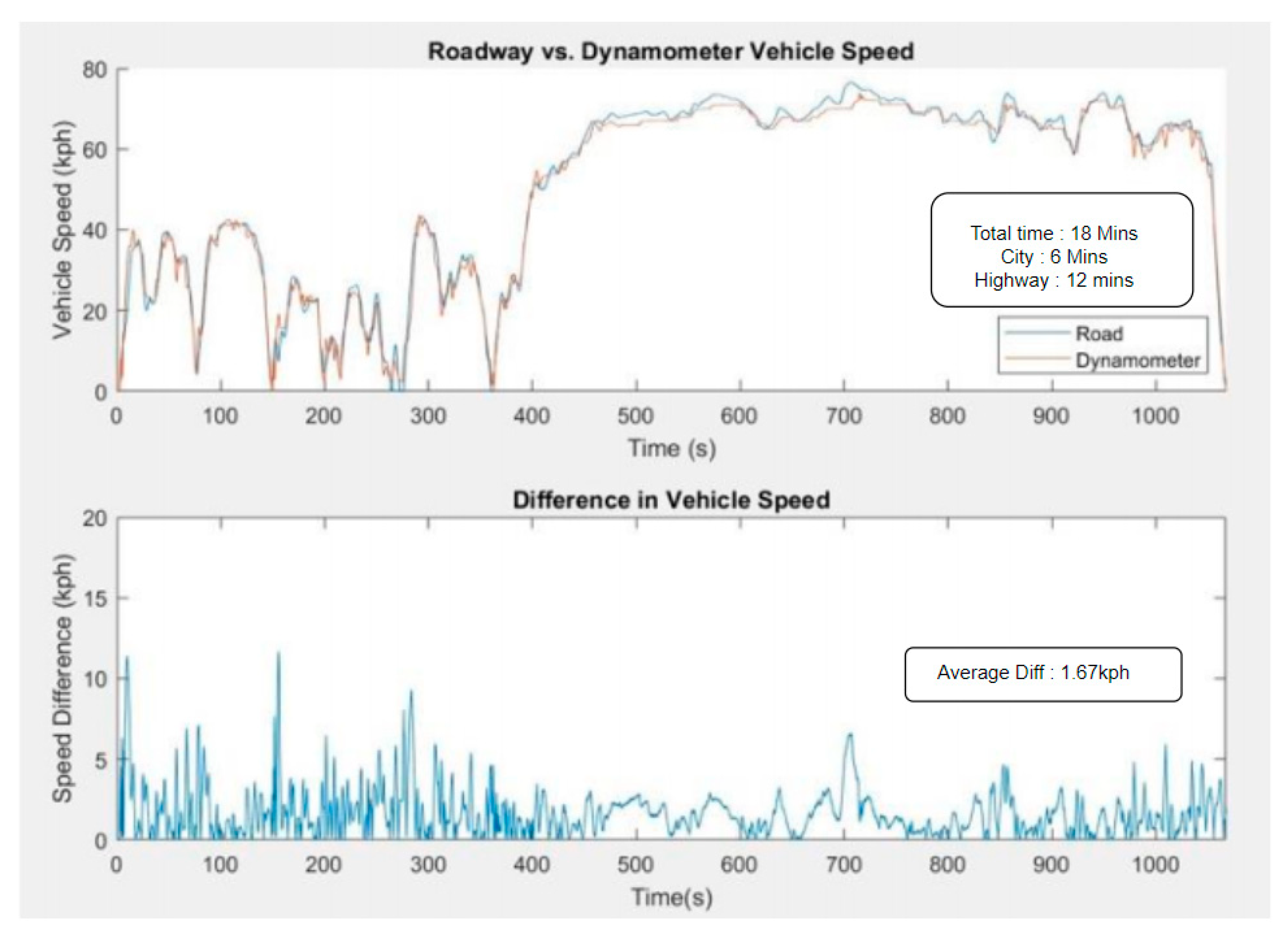
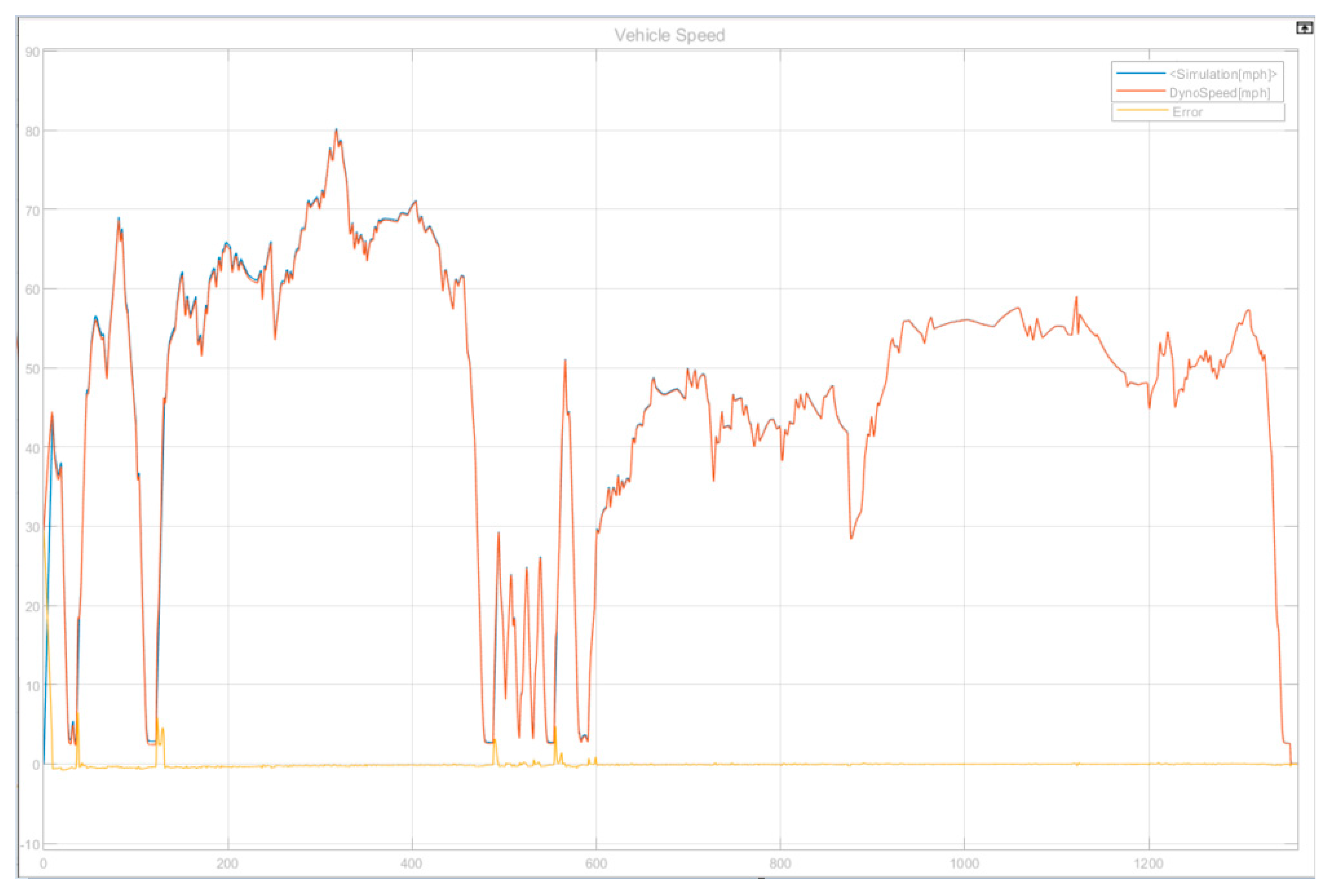
4. Validation of EV Model Simulation Results and Analysis
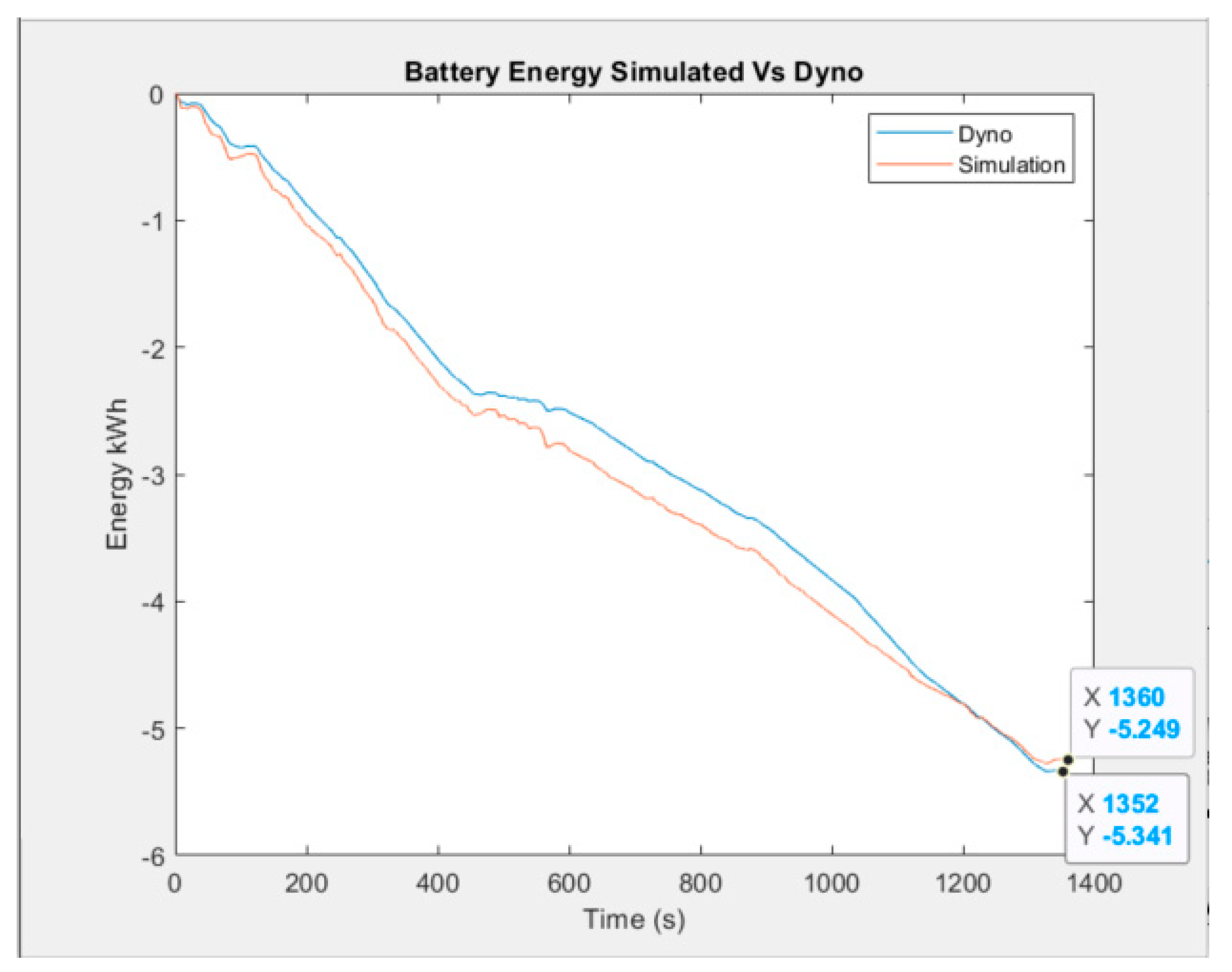
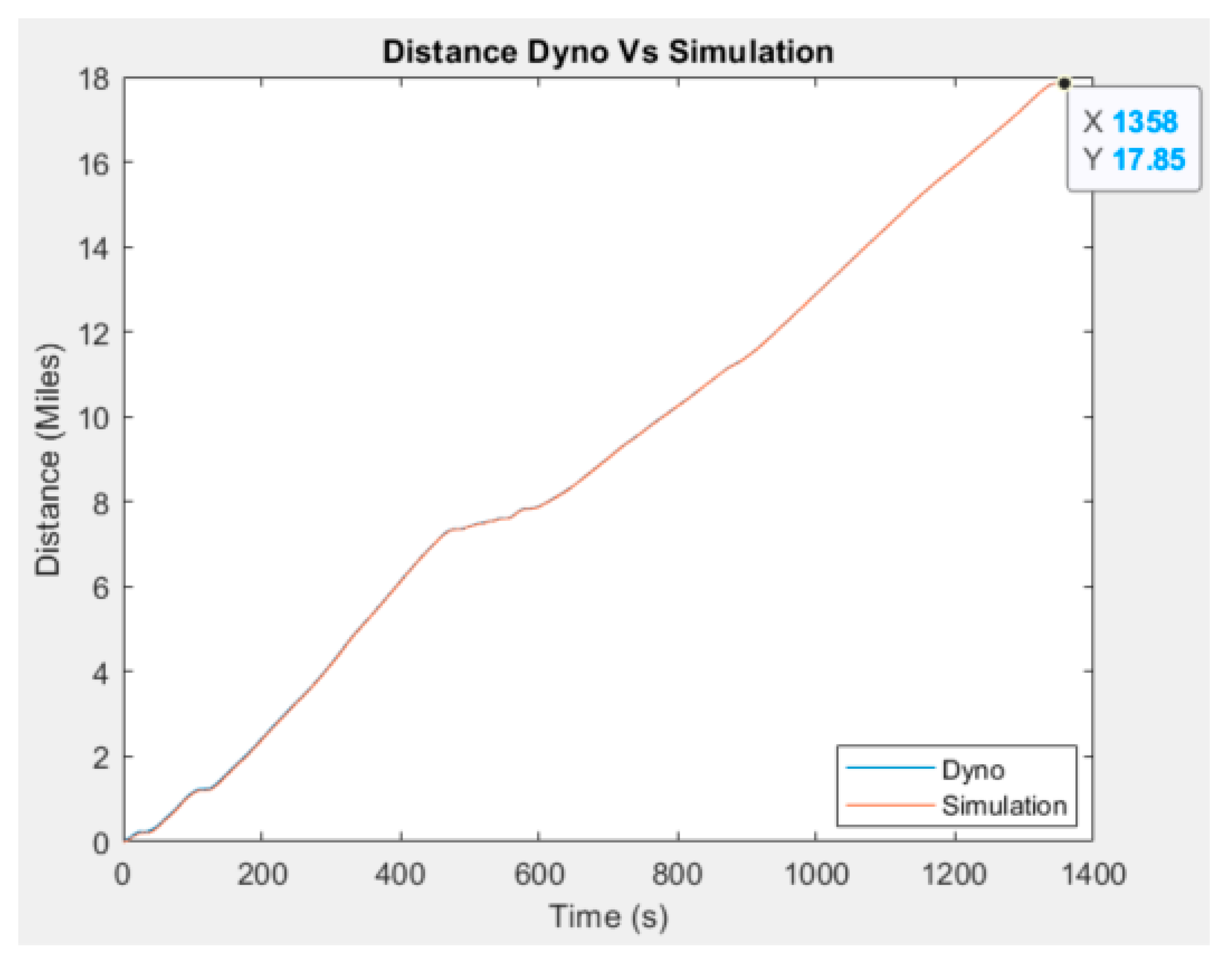
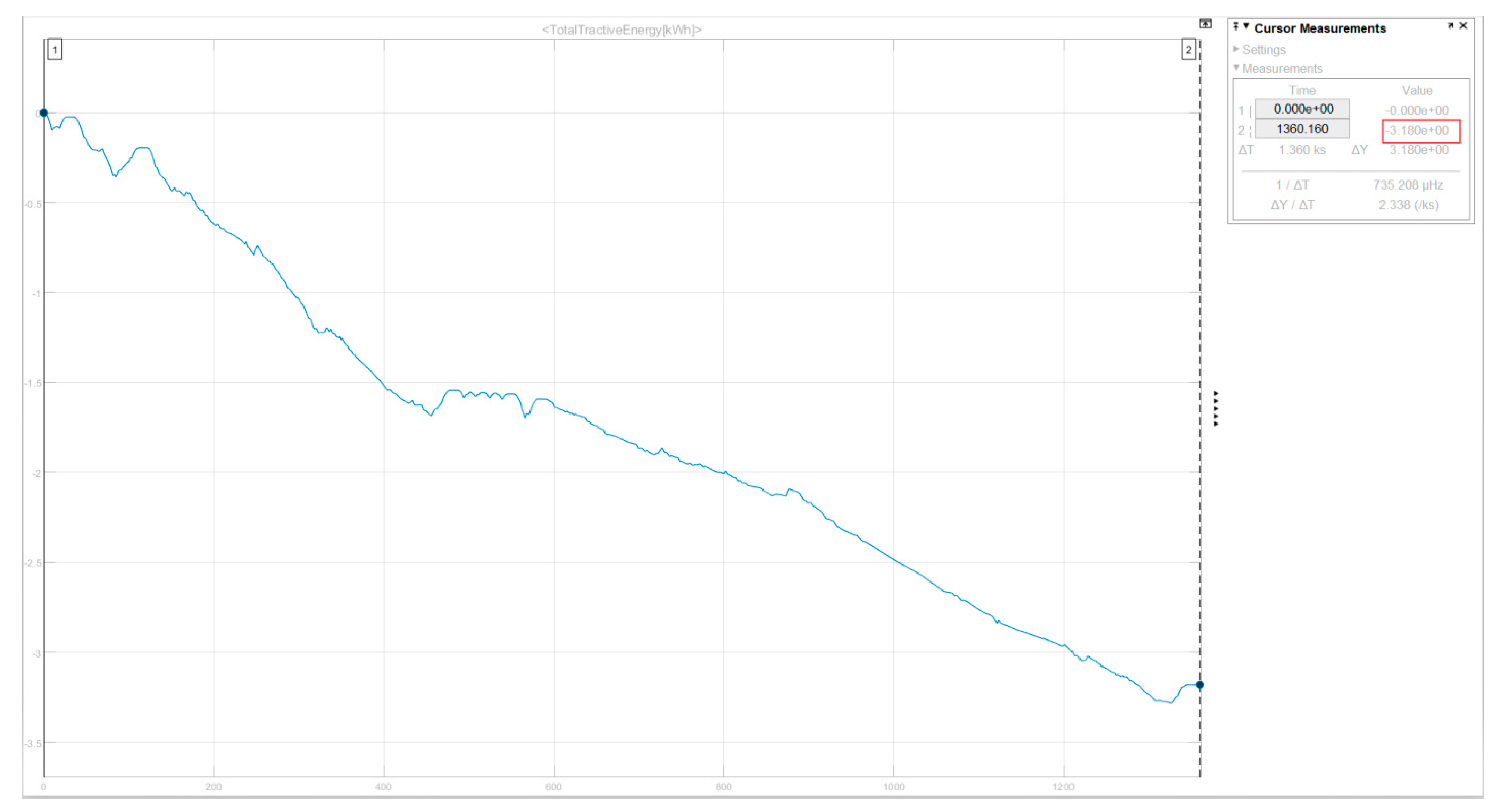
4.1. Energy Efficiency
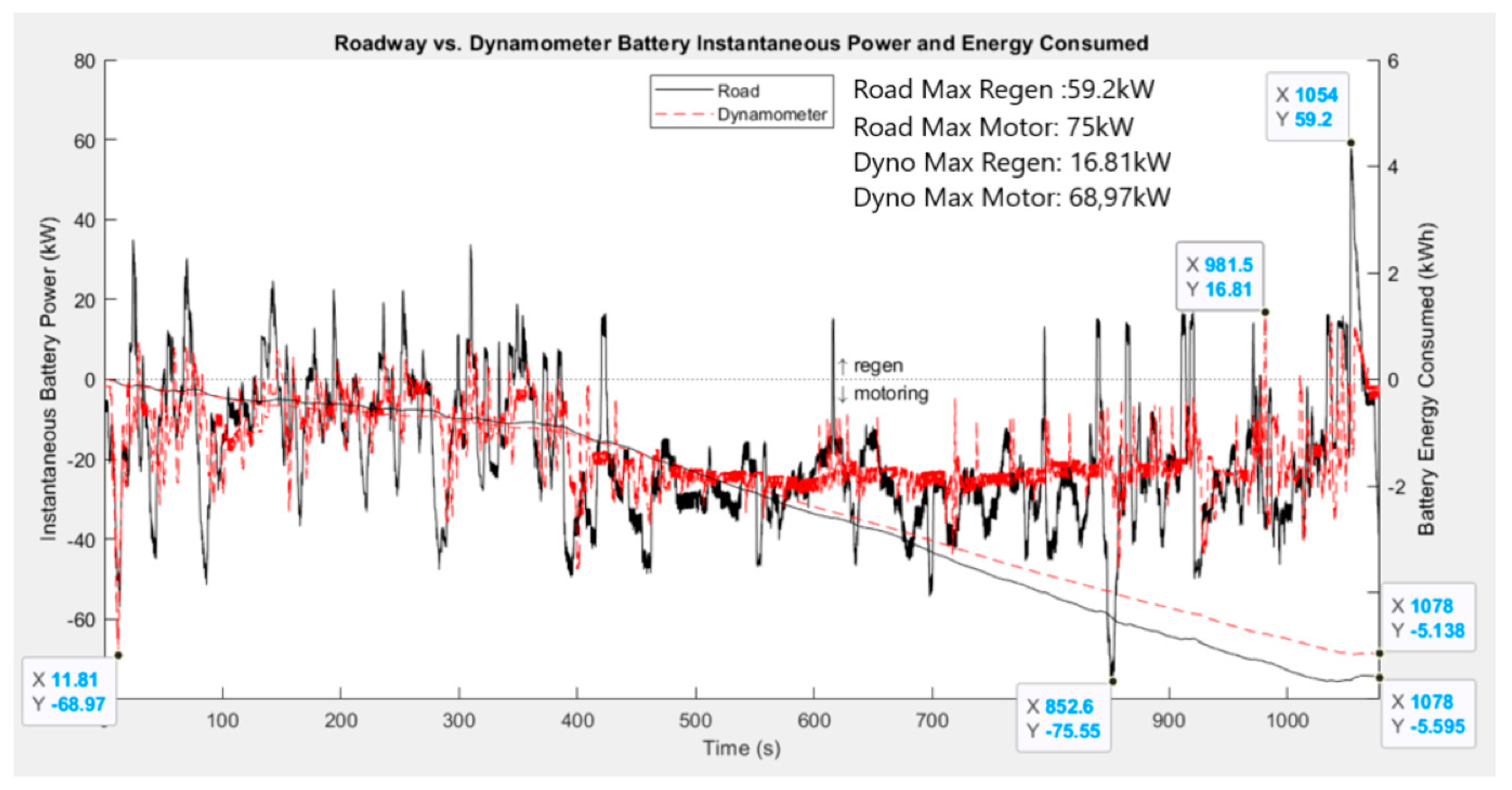
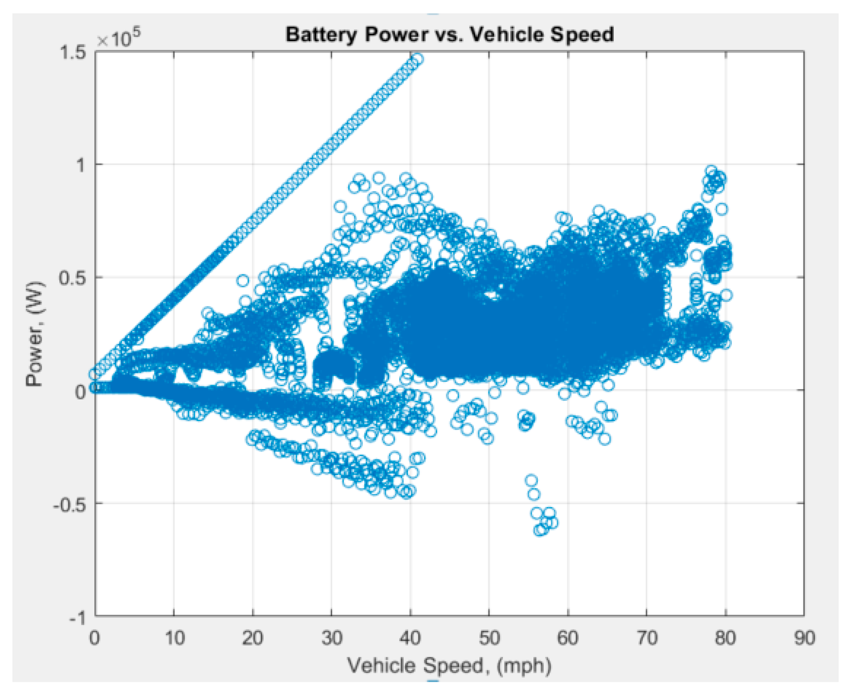
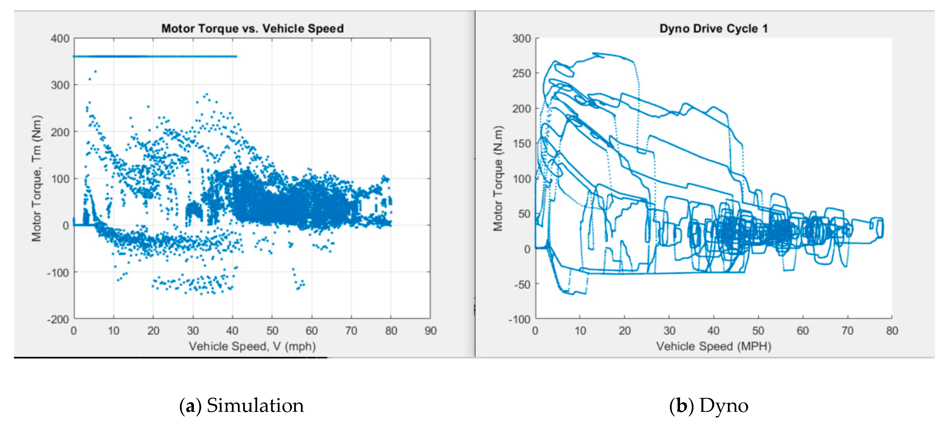
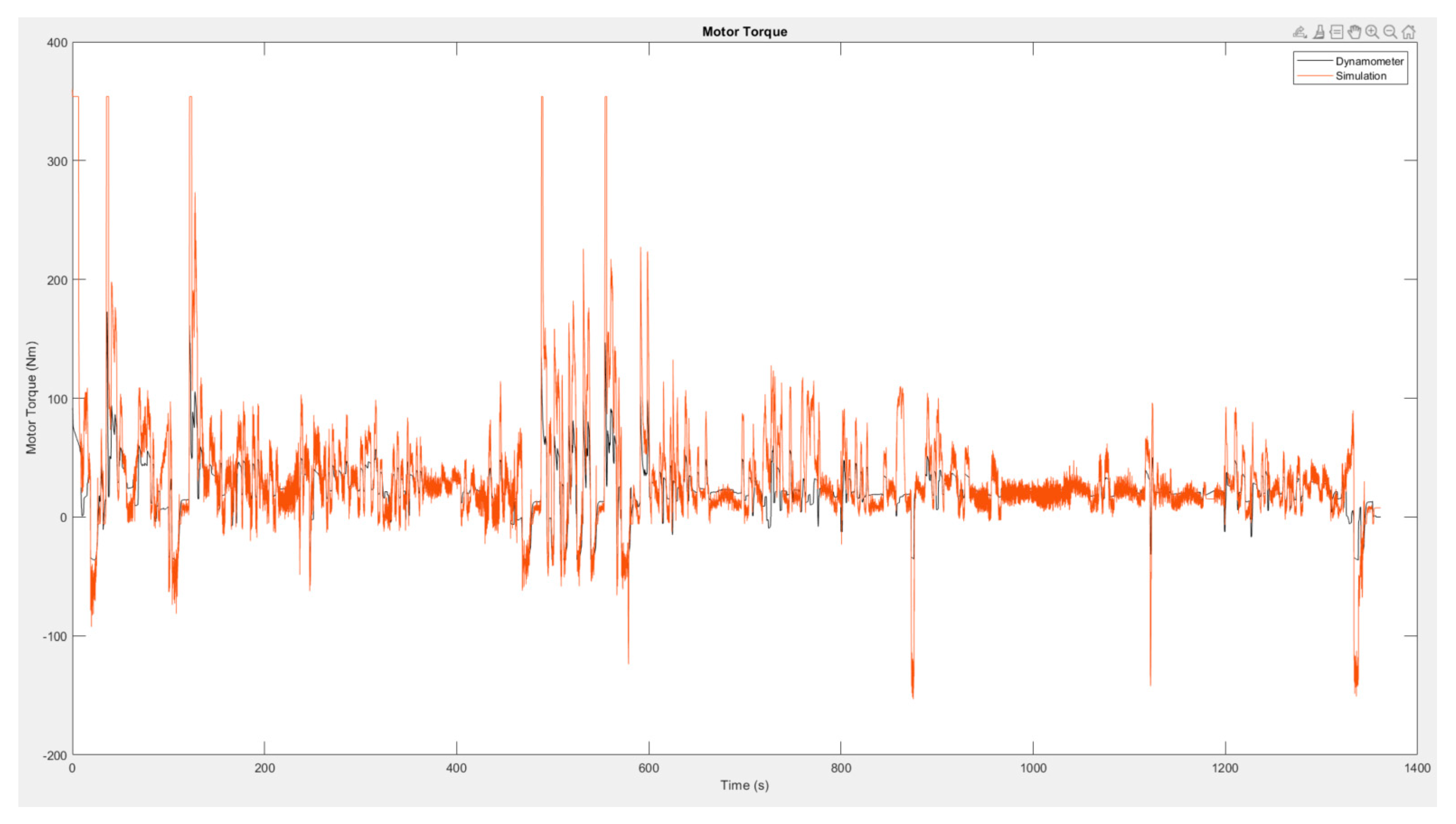
4.2. Motor Torque and Power
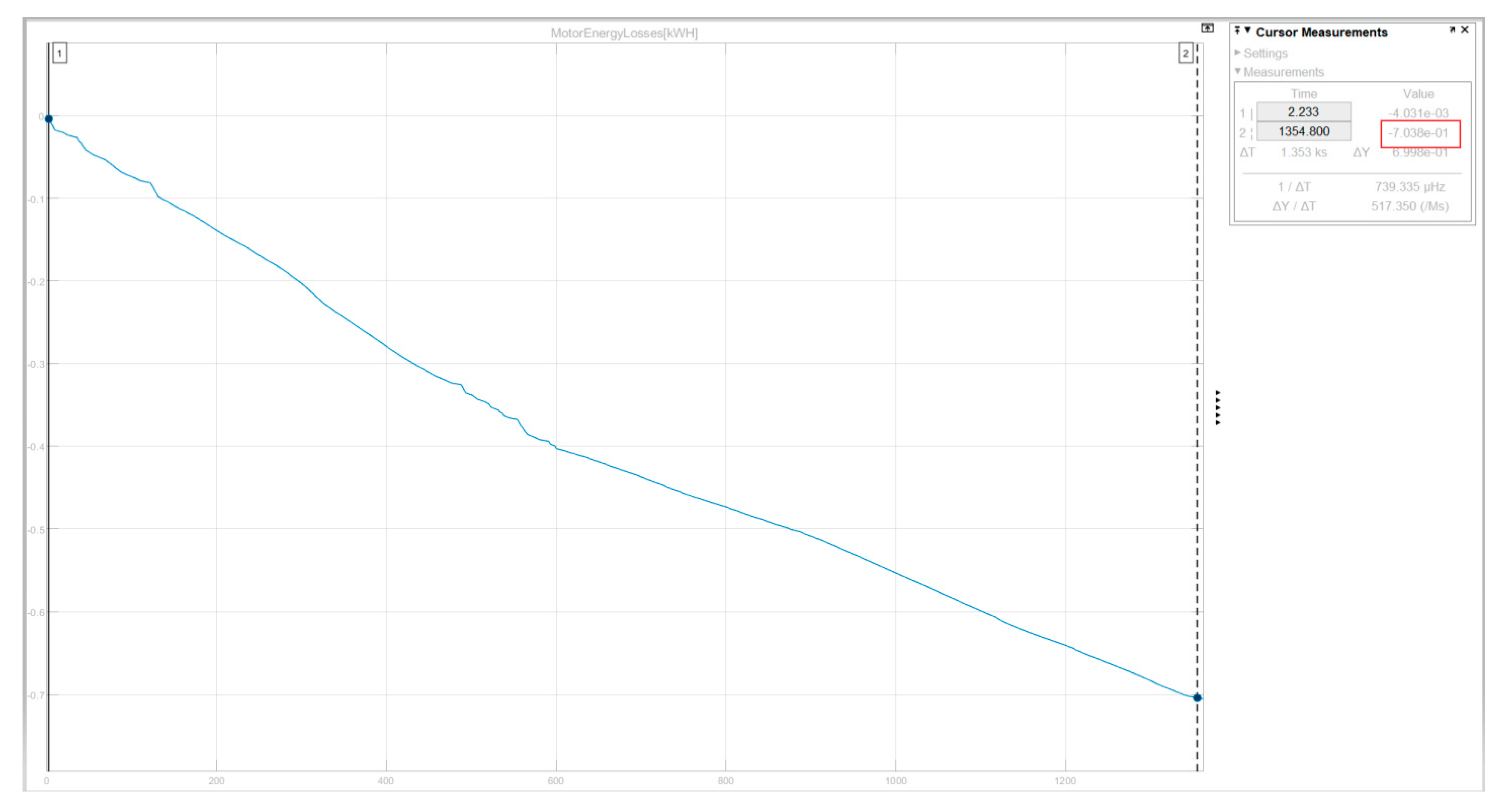
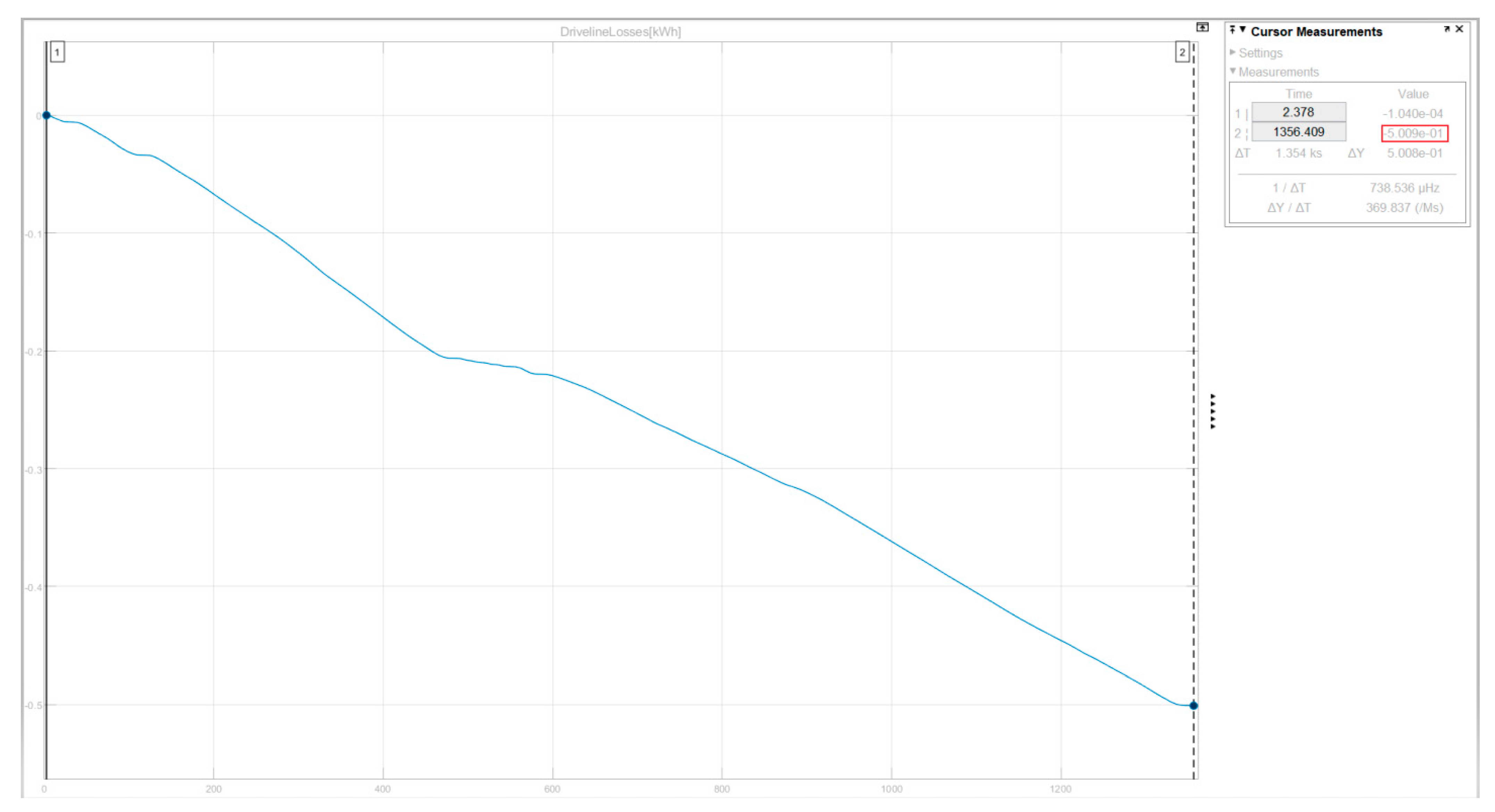
4.3. Loss Model
5. Conclusions
Author Contributions
Funding
Institutional Review Board Statement
Informed Consent Statement
Data Availability Statement
Conflicts of Interest
References
- BNEF. EV Sales 2020; Bloomberg New Energy Finance: New York, NY, USA, 2020. [Google Scholar]
- IEA. Global EV Outlook 2019; International Energy Agency: Paris, France, 2019. [Google Scholar]
- Kumar, R.R.; Alok, K. Adoption of electric vehicle: A literature review and prospects for sustainability. J. Clean. Prod. 2020, 253, 119911. [Google Scholar] [CrossRef]
- Traffic Safety Facts. 2016 Fatal Motor Vehicle Crashes: Overview; Research Note DOT HS 812 456; U.S. Department of Transportation, NHTSA’s National Center for Statistics and Analysis: Washington, DC, USA, 2017.
- Rowley, J.; Liu, A.; Sandry, S.; Gross, J.; Salvador, M.; Anton, C.; Fleming, C. Examining the driverless future: An analysis of human-caused vehicle accidents and development of an autonomous vehicle communication testbed. In Proceedings of the IEEE Systems and Information Engineering Design Symposium (SIEDS), Charlottesville, VA, USA, 27 April 2018. [Google Scholar]
- Kricke, C.; Hagel, S. A hybrid electric vehicle simulation model for component design and energy management optimization. In Proceedings of the FISITA World Automotive Congress, Paris, France, 27 September–1 October 1998. [Google Scholar]
- Auert, B.; Cheny, C.; Raison, B.; Berthon, A. Software tool for the simulation of the electro- mechanical behavior of a hybrid vehicle. In Proceedings of the Electric Vehicle Symposium 15, Brussels, Belgium, 29 September–3 October 1998. [Google Scholar]
- Onoda, S.; Emadi, A. PSIM-Based Modeling of Automotive Power Systems: Conventional, Electric, and Hybrid Electric Vehicles. IEEE Trans. Veh. Technol. 2004, 53, 390–400. [Google Scholar] [CrossRef]
- Amrhein, M.; Krein, P.T. Dynamic Simulation for Analysis of Hybrid Electric Vehicle System and Subsystem Interactions, Including Power Electronics. IEEE Trans. Veh. Technol. 2005, 54, 825–836. [Google Scholar] [CrossRef]
- Baisden, A.C.; Emadi, A. An ADVISOR based mode of a battery and an ultra-capacitor energy source for hybrid electric vehicles. IEEE Trans. Veh. Technol. 2004, 53, 199–205. [Google Scholar] [CrossRef]
- Gao, D.W.; Mi, C.; Emadi, A. Modeling and Simulation of Electric and Hybrid Vehicles. Proc. IEEE 2007, 95, 729–745. [Google Scholar] [CrossRef]
- Alam Chowdhury, M.S.; Al Mamun, K.A.; Rahman, A.M. Modelling and simulation of power system of battery, solar and fuel cell powered Hybrid Electric vehicle. In Proceedings of the 2016 3rd International Conference on Electrical Engineering and Information Communication Technology, Dhaka, Bangladesh, 22–24 September 2016; pp. 1–6. [Google Scholar] [CrossRef]
- Yaich, M.; Hachicha, M.R.; Ghariani, M. Modeling and simulation of electric and hybrid vehicles for recreational vehicle. In Proceedings of the 2015 16th International Conference on Sciences and Techniques of Automatic Control and Computer Engineering (STA), Monastir, Tunisia, 21–23 December 2015; pp. 181–187. [Google Scholar] [CrossRef]
- Zhou, J.; Shen, X.; Liu, D. Modeling and simulation for electric vehicle powertrain controls. In Proceedings of the 2014 IEEE Conference and Expo Transportation Electrification Asia-Pacific (ITEC Asia-Pacific), Beijing, China, 31 August–3 September 2014; pp. 1–4. [Google Scholar] [CrossRef]
- Tremblay, O.; Dessaint, L.; Dekkiche, A. A Generic Battery Model for the Dynamic Simulation of Hybrid Electric Vehicles. In Proceedings of the 2007 IEEE Vehicle Power and Propulsion Conference, Arlington, TX, USA, 9–12 September 2007; pp. 284–289. [Google Scholar] [CrossRef]
- MathWorks Student Competitions Team 2021. MATLAB and Simulink Racing Lounge: Vehicle Modeling. GitHub. Available online: https://github.com/mathworks/vehicle-modeling/releases/tag/v4.1.1 (accessed on 10 January 2021).
- Husain, I. Electric and Hybrid Vehicles: Design Fundamentals, 2nd ed.; CRC Press LLC: Boca Raton, FL, USA, 2010. [Google Scholar]
- Von Jouanne, A.; Adegbohun, J.; Collin, R.; Stephens, M.; Thayil, B.; Li, C.; Agamloh, E.; Yokochi, A. Electric Vehicle (EV) Chassis Dynamometer Testing. In Proceedings of the 2020 IEEE Energy Conversion Congress and Exposition (ECCE), Detroit, MI, USA, 11–15 October 2020; pp. 897–904. [Google Scholar] [CrossRef]
- SAE International. J1634 in Battery Electric Vehicle Energy Consumption and Range Test Procedure; SAE International: Warrendale, PA, USA, 2017. [Google Scholar]
- Agamloh, E.; Von Jouanne, A.; Yokochi, A. An Overview of Electric Machine Trends in Modern Electric Vehicles. Machines 2020, 8, 20. [Google Scholar] [CrossRef]
- Schauer, J.J.; Kleeman, M.J.; Cass, G.R.; Simoneit, B.R.T. Measurement of Emissions from Air Pollution Sources. 2. C1through C30Organic Compounds from Medium Duty Diesel Trucks. Environ. Sci. Technol. 1999, 33, 1578–1587. [Google Scholar] [CrossRef]
- Zielinska, B.; Sagebiel, J.; McDonald, J.D.; Whitney, K.; Lawson, D.R. Emission Rates and Comparative Chemical Composition from Selected In-Use Diesel and Gasoline-Fueled Vehicles. J. Air Waste Manag. Assoc. 2004, 54, 1138–1150. [Google Scholar] [CrossRef] [PubMed]
- Kogelschatz, U. Dielectric-barrier Discharges: Their History, Discharge Physics, and Industrial Applications. Plasma Chem. Plasma Proc. 2003, 23, 1–46. [Google Scholar] [CrossRef]


| Description | Value |
|---|---|
| Initial Acceleration (0–60 mph) | 7.5 s |
| Curb weight | 1616.15 kg |
| Motor power | 200 hp/150 kW |
| Motor torque | 266 lb.ft/360 Nm |
| Final drive ratio | 7.05:1 |
| Energy efficiency | 300 Wh/mile |
| Battery capacity | 53 kWh |
| Top speed | 93 mph |
| Aerodynamic drag coefficient | 0.308 |
| Parameter | Unit | Description | Value |
|---|---|---|---|
| Air Density | 1.23 | ||
| - | Drag coefficient | 0.38 | |
| Vehicle frontal Area | 2.1 | ||
| Vehicle Speed | - | ||
| Vehicle acceleration | - | ||
| Vehicle inertial mass | 1678.30 | ||
| Vehicle Mass | 1616.15 | ||
| Gravity | 9.81 | ||
| Road angle | 0 | ||
| - | Rolling resistance coefficient | 0.01 |
| Parameter | Units | Description | Value |
|---|---|---|---|
| Maximum motor torque | 450 | ||
| Motor base speed | 834 | ||
| Motor loss constant | 0.12 | ||
| Motor loss constant | 0.01 | ||
| Motor loss constant | 1.2 × 10⁻⁵ | ||
| Motor loss constant | 600 |
Publisher’s Note: MDPI stays neutral with regard to jurisdictional claims in published maps and institutional affiliations. |
© 2021 by the authors. Licensee MDPI, Basel, Switzerland. This article is an open access article distributed under the terms and conditions of the Creative Commons Attribution (CC BY) license (http://creativecommons.org/licenses/by/4.0/).
Share and Cite
Adegbohun, F.; von Jouanne, A.; Phillips, B.; Agamloh, E.; Yokochi, A. High Performance Electric Vehicle Powertrain Modeling, Simulation and Validation. Energies 2021, 14, 1493. https://doi.org/10.3390/en14051493
Adegbohun F, von Jouanne A, Phillips B, Agamloh E, Yokochi A. High Performance Electric Vehicle Powertrain Modeling, Simulation and Validation. Energies. 2021; 14(5):1493. https://doi.org/10.3390/en14051493
Chicago/Turabian StyleAdegbohun, Feyijimi, Annette von Jouanne, Ben Phillips, Emmanuel Agamloh, and Alex Yokochi. 2021. "High Performance Electric Vehicle Powertrain Modeling, Simulation and Validation" Energies 14, no. 5: 1493. https://doi.org/10.3390/en14051493
APA StyleAdegbohun, F., von Jouanne, A., Phillips, B., Agamloh, E., & Yokochi, A. (2021). High Performance Electric Vehicle Powertrain Modeling, Simulation and Validation. Energies, 14(5), 1493. https://doi.org/10.3390/en14051493