
A Multi-Objective Life Cycle Optimization Model of an Integrated Algal Biorefinery toward a Sustainable Circular Bioeconomy Considering Resource Recirculation

 , ,
, ,  and
and 
Abstract
1. Introduction
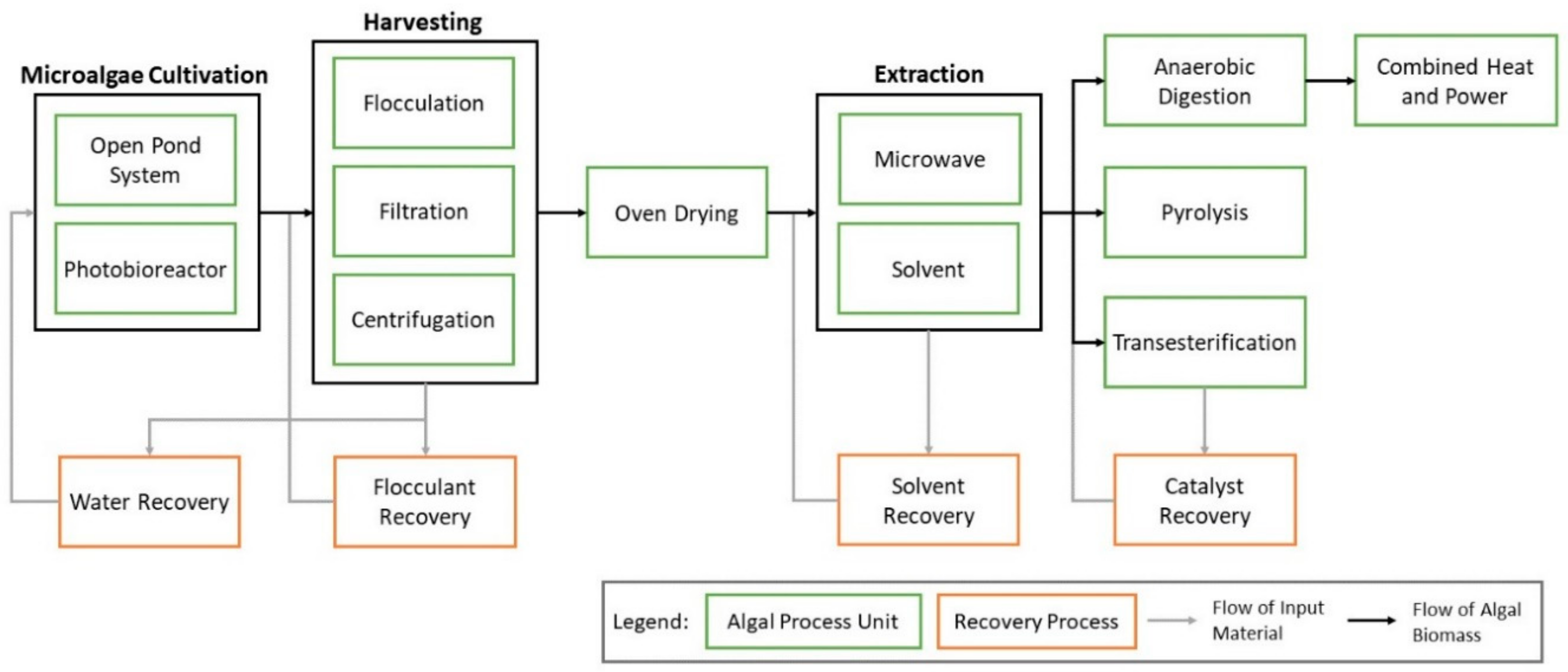
2. System Definition
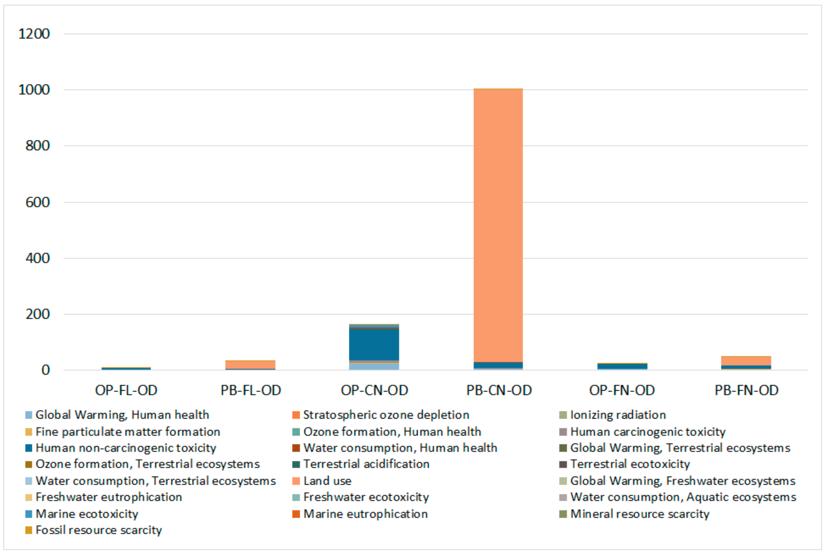
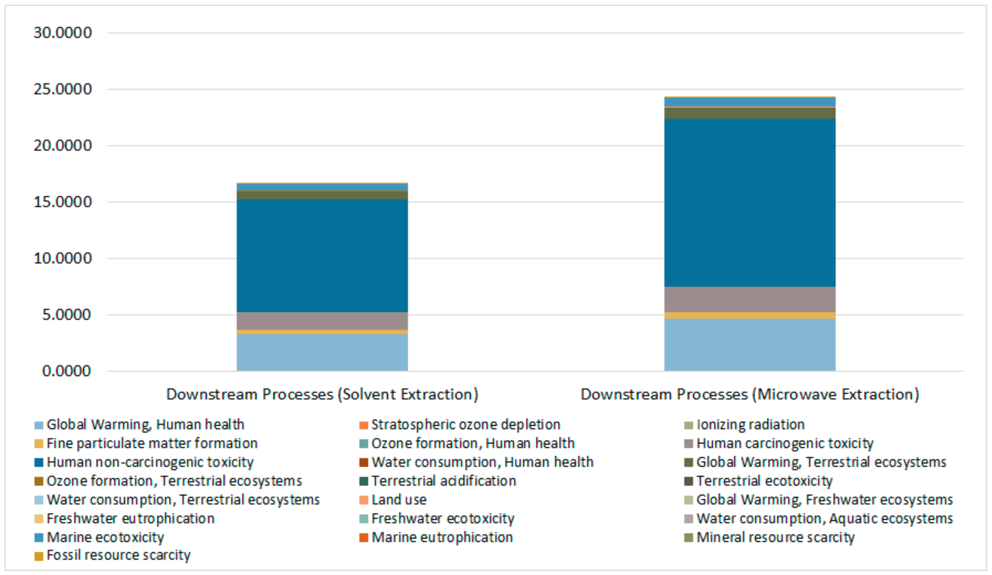
3. Life Cycle Assessment
4. Model Formulation
4.1. Model Assumptions
- All parameters considered in this model are deterministic and known with certainty.
- The outputs produced by the facility are transported to customers at the same time.
- Processing of algal biomass in all facilities is instantaneous.
4.2. Optimization Model
4.2.1. Objective Functions
4.2.2. Constraints
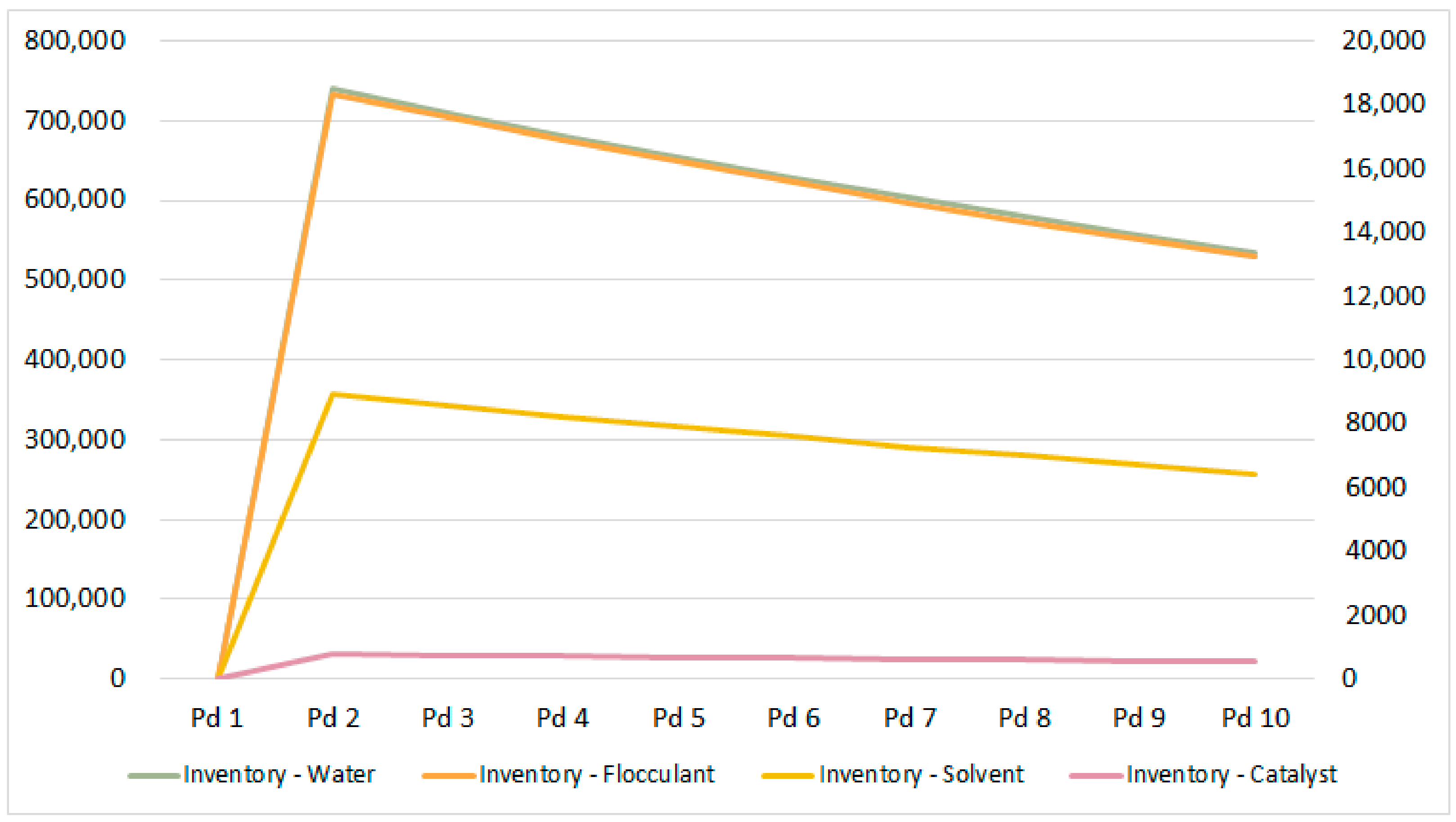
5. Model Validation
5.1. Profit Maximization
5.2. Impact Minimization
5.3. Multi-Objective Model
6. Scenario Analysis
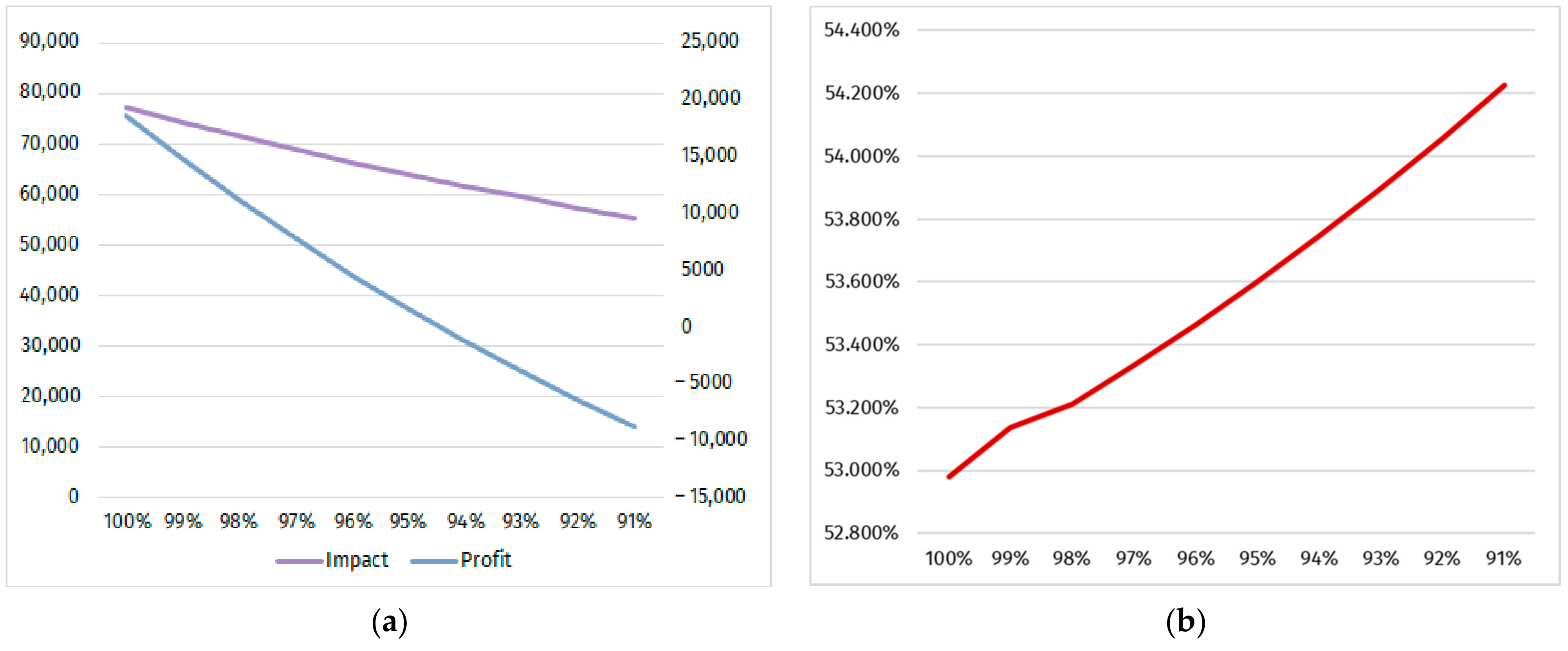
6.1. Impact of Process Unit Efficiencies
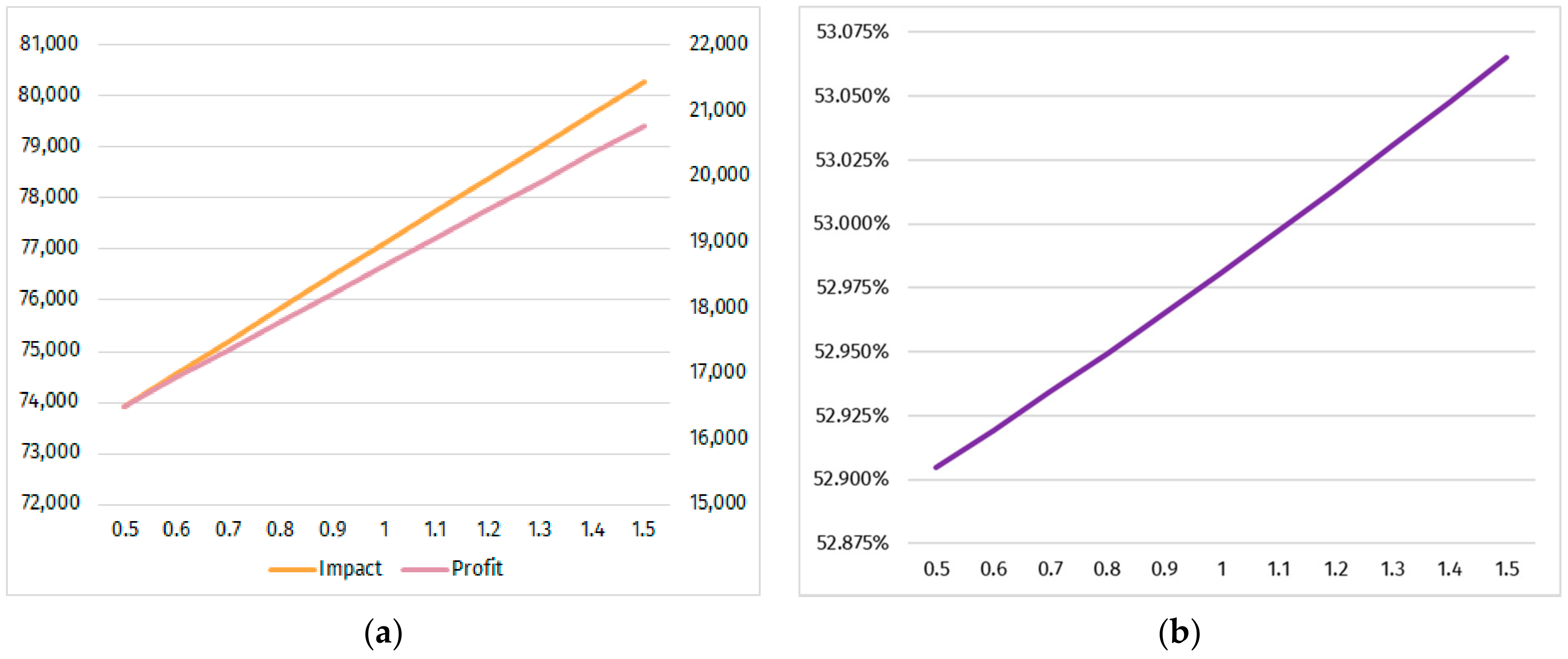
6.2. Impact of Demand Fluctuations
7. Conclusions and Recommendations
Author Contributions
Funding
Conflicts of Interest
Appendix A

| Demand (kg) | Selling Price (USD/kg) | |
|---|---|---|
| Biodiesel | 25,000 | 12.50 |
| Glycerol | 2500 | 0.78 |
| Biochar | 1000 | 0.50 |
| Fertilizer | 200 | 0.25 |
| Purchase Cost (USD/kg) | Inventory Cost (USD/kg/pd) | |
|---|---|---|
| Water | 0.367 | 0.15 |
| Potassium sulfate | 0.12 | 0.15 |
| Hexane | 0.41 | 0.15 |
| Sulfuric acid | 0.74 | 0.15 |
| Fixed Cost (USD) | Operating Cost (USD) | |
|---|---|---|
| Open Pond | 734,713.76 | 0.50 |
| Photobioreactor | 1,192,058.79 | 0.50 |
| Flocculation | 923,823.86 | 0.50 |
| Centrifugation | 285,617.51 | 0.50 |
| Filtration | 807,400.00 | 0.50 |
| Oven Drying | 632,120.00 | 0.50 |
| Solvent Extraction | 720,000.00 | 0.50 |
| Microwave Extraction | 936,000.00 | 0.50 |
| Transesterification | 1,050,441.71 | 0.50 |
| Pyrolysis | 357,760 | 0.50 |
| Anaerobic Digestion | 693,600 | 0.50 |
| Combined Heat and Power | 459,000 | 0.25 |
| Stages | Material | OP-FL-SO | OP-CN-SO | OP-FN-SO | OP-FL-MI | OP-CN-MI | OP-FN-MI |
|---|---|---|---|---|---|---|---|
| Cultivation—Open Pond | Water (kg) | 6.4852 | 221.7602 | 6.3385 | 1.7546 | 59.9993 | 1.7150 |
| Urea (g) | 2.5779 | 88.1497 | 2.5196 | 0.6975 | 23.8497 | 0.6817 | |
| Diammonium phosphate (g) | 2.3185 | 79.2793 | 2.2660 | 0.6273 | 21.4498 | 0.6131 | |
| Electricity (MJ) | 0.3599 | 12.3077 | 0.3518 | 0.0974 | 3.3300 | 0.0952 | |
| * Algal broth (kg) | 6.6203 | 226.3802 | 6.4706 | 1.7912 | 61.2493 | 1.7507 | |
| Harvesting—Flocculation | Potassium sulfate (kg) | 0.0794 | 0.0215 | ||||
| Electricity (MJ) | 7.7385 | 2.0937 | |||||
| Algal broth (kg) | 6.6203 | 1.7912 | |||||
| * Wet biomass (kg) | 5.4353 | 1.4706 | |||||
| Harvesting—Centrifugation | Chitosan (g) | 45.9690 | 12.4374 | ||||
| Electricity (MJ) | 12.4740 | 3.3750 | |||||
| Algal broth (kg) | 226.3802 | 61.2493 | |||||
| * Wet biomass (kg) | 5.4353 | 1.4706 | |||||
| Harvesting—Filtration | Electricity (MJ) | 190.2355 | 51.4700 | ||||
| Algal broth (kg) | 6.4706 | 1.7507 | |||||
| * Wet biomass (kg) | 5.4353 | 1.4706 | |||||
| Oven Drying | Wet biomass (kg) | 5.4353 | 5.4353 | 5.4353 | 1.4706 | 1.4706 | 1.4706 |
| Heat (MJ) | 62.4516 | 62.4516 | 62.4516 | 16.8969 | 16.8969 | 16.8969 | |
| * Dry biomass (kg) | 4.6200 | 4.6200 | 4.6200 | 1.2500 | 1.2500 | 1.2500 | |
| Extraction—Solvent | Hexane (g) | 2.9568 | 2.9568 | 2.9568 | |||
| Electricity (MJ) | 0.3326 | 0.3326 | 0.3326 | ||||
| Heat (MJ) | 2.3100 | 2.3100 | 2.3100 | ||||
| Dry biomass (kg) | 4.6200 | 4.6200 | 4.6200 | ||||
| * Algal oil (g) | 1049.9884 | 1049.9884 | 1049.9884 | ||||
| * Liquid residue (g) | 170.0000 | 170.0000 | 170.0000 | ||||
| * Solid residue (g) | 40.0000 | 40.0000 | 40.0000 | ||||
| Extraction—Microwave | Electricity (MJ) | 36.7496 | 36.7496 | 36.7496 | |||
| Dry biomass (kg) | 1.2500 | 1.2500 | 1.2500 | ||||
| * Algal oil (kg) | 1.0500 | 1.0500 | 1.0500 | ||||
| * Liquid residue (g) | 45.9951 | 45.9951 | 45.9951 | ||||
| * Solid residue (g) | 10.8224 | 10.8224 | 10.8224 | ||||
| Transesterification | Algal oil (g) | 1049.9884 | 1049.9884 | 1049.9884 | 1049.9884 | 1049.9884 | 1049.9884 |
| Methanol (g) | 124.8787 | 124.8787 | 124.8787 | 124.8787 | 124.8787 | 124.8787 | |
| Sodium hydroxide (g) | 10.4874 | 10.4874 | 10.4874 | 10.4874 | 10.4874 | 10.4874 | |
| Sulfuric acid (g) | 15.8004 | 15.8004 | 15.8004 | 15.8004 | 15.8004 | 15.8004 | |
| Electricity (MJ) | 0.1663 | 0.1663 | 0.1663 | 0.1663 | 0.1663 | 0.1663 | |
| Heat (MJ) | 5.5902 | 5.5902 | 5.5902 | 5.5902 | 5.5902 | 5.5902 | |
| Water (kg) | 0.1386 | 0.1386 | 0.1386 | 0.1386 | 0.1386 | 0.1386 | |
| * Biodiesel (g) | 1000.0000 | 1000.0000 | 1000.0000 | 1000.0000 | 1000.0000 | 1000.0000 | |
| * Glycerol (g) | 113.2825 | 113.2825 | 113.2825 | 113.2825 | 113.2825 | 113.2825 | |
| Pyrolysis | Solid residue (g) | 40.0000 | 40.0000 | 40.0000 | 10.8224 | 10.8224 | 10.8224 |
| Heat (MJ) | 6.4168 | 6.4168 | 6.4168 | 1.7361 | 1.7361 | 1.7361 | |
| * Biochar (g) | 5.9970 | 5.9970 | 5.9970 | 1.6225 | 1.6225 | 1.6225 | |
| Anaerobic Digestion | Liquid residue (g) | 170.0000 | 170.0000 | 170.0000 | 45.9951 | 45.9951 | 45.9951 |
| Electricity (MJ) | 54.7260 | 54.7260 | 54.7260 | 14.8066 | 14.8066 | 14.8066 | |
| Heat (MJ) | 416.2671 | 416.2671 | 416.2671 | 112.6250 | 112.6250 | 112.6250 | |
| * Methane (g) | 19.4064 | 19.4064 | 19.4064 | 5.2506 | 5.2506 | 5.2506 | |
| * Fertilizer (g) | 69.8428 | 69.8428 | 69.8428 | 18.8966 | 18.8966 | 18.8966 | |
| Combined Heat and Power | Methane (g) | 19.4064 | 19.4064 | 19.4064 | 5.2506 | 5.2506 | 5.2506 |
| * Electricity (MJ) | 0.2156 | 0.2156 | 0.2156 | 0.0583 | 0.0583 | 0.0583 | |
| * Heat (MJ) | 0.4097 | 0.4097 | 0.4097 | 0.1108 | 0.1108 | 0.1108 |
| Stages | Input | PB-FL-SO | PB-CN-SO | PB-FN-SO | PB-FL-MI | PB-CN-MI | PB-FN-MI |
|---|---|---|---|---|---|---|---|
| Cultivation—Open Pond | Water (kg) | 5.6105 | 191.8476 | 5.4836 | 1.5180 | 51.9062 | 1.4836 |
| Chicken compost (kg) | 0.2244 | 7.6739 | 0.2193 | 0.0607 | 2.0762 | 0.0593 | |
| Atmospheric air (kg) | 0.2244 | 7.6739 | 0.2193 | 0.0607 | 2.0762 | 0.0593 | |
| Inoculum (kg) | 0.5610 | 19.1848 | 0.5484 | 0.1518 | 5.1906 | 0.1484 | |
| Electricity (MJ) | 5.5890 | 191.1152 | 5.4626 | 1.5122 | 51.7080 | 1.4780 | |
| * Algal broth (kg) | 6.6203 | 226.3802 | 6.4706 | 1.7912 | 61.2493 | 1.7507 | |
| Harvesting—Flocculation | Potassium sulfate (kg) | 0.0794 | 0.0215 | ||||
| Electricity (MJ) | 7.7385 | 2.0937 | |||||
| Algal broth (kg) | 6.6203 | 1.7912 | |||||
| * Wet biomass (kg) | 5.4353 | 1.4706 | |||||
| Harvesting—Centrifugation | Chitosan (g) | 45.9690 | 12.4374 | ||||
| Electricity (MJ) | 12.4740 | 3.3750 | |||||
| Algal broth (kg) | 226.3802 | 61.2493 | |||||
| * Wet biomass (kg) | 5.4353 | 1.4706 | |||||
| Harvesting—Filtration | Electricity (MJ) | 190.2355 | 51.4700 | ||||
| Algal broth (kg) | 6.4706 | 1.7507 | |||||
| * Wet biomass (kg) | 5.4353 | 1.4706 | |||||
| Oven Drying | Wet biomass (kg) | 5.4353 | 5.4353 | 5.4353 | 1.4706 | 1.4706 | 1.4706 |
| Heat (MJ) | 62.4516 | 62.4516 | 62.4516 | 16.8969 | 16.8969 | 16.8969 | |
| * Dry biomass (kg) | 4.6200 | 4.6200 | 4.6200 | 1.2500 | 1.2500 | 1.2500 | |
| Extraction—Solvent | Hexane (g) | 2.9568 | 2.9568 | 2.9568 | |||
| Electricity (MJ) | 0.3326 | 0.3326 | 0.3326 | ||||
| Heat (MJ) | 2.3100 | 2.3100 | 2.3100 | ||||
| Dry biomass (kg) | 4.6200 | 4.6200 | 4.6200 | ||||
| * Algal oil (g) | 1049.9884 | 1049.9884 | 1049.9884 | ||||
| * Liquid residue (g) | 170.0000 | 170.0000 | 170.0000 | ||||
| * Solid residue (g) | 40.0000 | 40.0000 | 40.0000 | ||||
| Extraction—Microwave | Electricity (MJ) | 36.7496 | 36.7496 | 36.7496 | |||
| Dry biomass (kg) | 1.2500 | 1.2500 | 1.2500 | ||||
| * Algal oil (kg) | 1.0500 | 1.0500 | 1.0500 | ||||
| * Liquid residue (g) | 45.9951 | 45.9951 | 45.9951 | ||||
| * Solid residue (g) | 10.8224 | 10.8224 | 10.8224 | ||||
| Transesterification | Algal oil (g) | 1049.9884 | 1049.9884 | 1049.9884 | 1049.9884 | 1049.9884 | 1049.9884 |
| Methanol (g) | 124.8787 | 124.8787 | 124.8787 | 124.8787 | 124.8787 | 124.8787 | |
| Sodium hydroxide (g) | 10.4874 | 10.4874 | 10.4874 | 10.4874 | 10.4874 | 10.4874 | |
| Sulfuric acid (g) | 15.8004 | 15.8004 | 15.8004 | 15.8004 | 15.8004 | 15.8004 | |
| Electricity (MJ) | 0.1663 | 0.1663 | 0.1663 | 0.1663 | 0.1663 | 0.1663 | |
| Heat (MJ) | 5.5902 | 5.5902 | 5.5902 | 5.5902 | 5.5902 | 5.5902 | |
| Water (kg) | 0.1386 | 0.1386 | 0.1386 | 0.1386 | 0.1386 | 0.1386 | |
| * Biodiesel (g) | 1000.0000 | 1000.0000 | 1000.0000 | 1000.0000 | 1000.0000 | 1000.0000 | |
| * Glycerol (g) | 113.2825 | 113.2825 | 113.2825 | 113.2825 | 113.2825 | 113.2825 | |
| Pyrolysis | Solid residue (g) | 40.0000 | 40.0000 | 40.0000 | 10.8224 | 10.8224 | 10.8224 |
| Heat (MJ) | 6.4168 | 6.4168 | 6.4168 | 1.7361 | 1.7361 | 1.7361 | |
| * Biochar (g) | 5.9970 | 5.9970 | 5.9970 | 1.6225 | 1.6225 | 1.6225 | |
| Anaerobic Digestion | Liquid residue (g) | 170.0000 | 170.0000 | 170.0000 | 45.9951 | 45.9951 | 45.9951 |
| Electricity (MJ) | 54.7260 | 54.7260 | 54.7260 | 14.8066 | 14.8066 | 14.8066 | |
| Heat (MJ) | 416.2671 | 416.2671 | 416.2671 | 112.6250 | 112.6250 | 112.6250 | |
| * Methane (g) | 19.4064 | 19.4064 | 19.4064 | 5.2506 | 5.2506 | 5.2506 | |
| * Fertilizer (g) | 69.8428 | 69.8428 | 69.8428 | 18.8966 | 18.8966 | 18.8966 | |
| Combined Heat and Power | Methane (g) | 19.4064 | 19.4064 | 19.4064 | 5.2506 | 5.2506 | 5.2506 |
| * Electricity (MJ) | 0.2156 | 0.2156 | 0.2156 | 0.0583 | 0.0583 | 0.0583 | |
| * Heat (MJ) | 0.4097 | 0.4097 | 0.4097 | 0.1108 | 0.1108 | 0.1108 |
| Category | Normalization Factor | Weighting Factor |
|---|---|---|
| Damage to human health | 11.2 | 400 |
| Damage to ecosystems | 1186 | 400 |
| Damage to resource availability | 0.000357 | 200 |
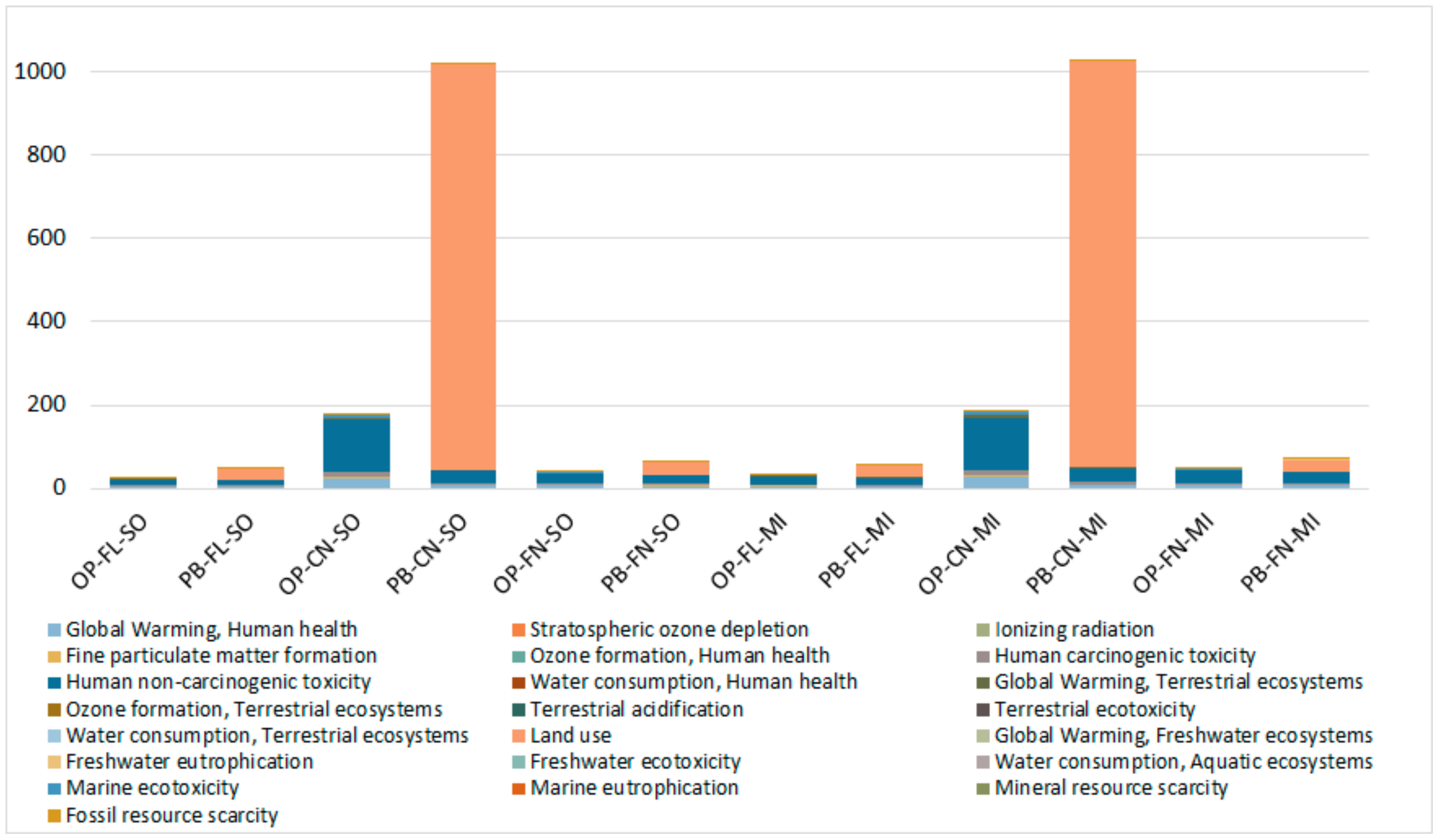
| Impact Category | OP-FL-SO | OP-CN-SO | OP-FN-SO | OP-FL-MI | OP-CN-MI | OP-FN-MI | PB-FL-SO | PB-CN-SO | PB-FN-SO | PB-FL-MI | PB-CN-MI | PB-FN-MI |
|---|---|---|---|---|---|---|---|---|---|---|---|---|
| Global Warming, Human health | 4.4227 | 3.9009 | 24.8744 | 7.0341 | 6.3919 | 5.8820 | 5.7478 | 5.2261 | 26.1995 | 8.3593 | 7.7171 | 7.2071 |
| Stratospheric ozone depletion | 1.79 × 10⁻⁴ | 5.37 × 10⁻³ | 1.42 × 10⁻³ | 1.79 × 10⁻¹ | 2.83 × 10⁻⁴ | 5.36 × 10⁻³ | 2.35 × 10⁻⁴ | 5.43 × 10⁻³ | 1.48 × 10⁻³ | 1.79 × 10⁻¹ | 3.39 × 10⁻⁴ | 5.42 × 10⁻³ |
| Ionizing radiation | 1.14 × 10⁻⁴ | 7.14 × 10⁻⁵ | 2.01 × 10⁻³ | 5.75 × 10⁻⁴ | 1.39 × 10⁻⁴ | 9.79 × 10⁻⁵ | 1.33 × 10⁻⁴ | 9.05 × 10⁻⁵ | 2.03 × 10⁻³ | 5.94 × 10⁻⁴ | 1.58 × 10⁻⁴ | 1.17 × 10⁻⁴ |
| Fine particulate matter formation | 0.5600 | 0.4905 | 3.3394 | 0.9656 | 0.8982 | 0.8303 | 0.7441 | 0.6747 | 3.5236 | 1.1497 | 1.0824 | 1.0145 |
| Ozone formation, Human health | 7.96 × 10⁻⁴ | 7.66 × 10⁻⁴ | 3.85 × 10⁻³ | 2.81 × 10⁻³ | 1.18 × 10⁻³ | 1.15 × 10⁻³ | 1.05 × 10⁻³ | 1.02 × 10⁻³ | 4.10 × 10⁻³ | 3.06 × 10⁻³ | 1.43 × 10⁻³ | 1.40 × 10⁻³ |
| Human carcinogenic toxicity | 2.1092 | 1.8749 | 12.1635 | 4.1494 | 3.6177 | 3.3886 | 2.8535 | 2.6191 | 12.9078 | 4.8936 | 4.3619 | 4.1329 |
| Human non-carcinogenic toxicity | 14.7170 | 11.9791 | 122.8033 | 29.1829 | 24.7466 | 22.0706 | 19.5436 | 16.8058 | 127.6299 | 34.0095 | 29.5732 | 26.8973 |
| Water consumption, Human health | 7.01 × 10⁻³ | 5.32 × 10⁻⁴ | 2.28 × 10⁻¹ | 6.33 × 10⁻³ | 6.93 × 10⁻³ | 5.98 × 10⁻⁴ | 7.12 × 10⁻³ | 6.44 × 10⁻⁴ | 2.28 × 10⁻¹ | 6.44 × 10⁻³ | 7.04 × 10⁻³ | 7.10 × 10⁻⁴ |
| Global Warming, Terrestrial ecosystems | 0.9381 | 0.8274 | 5.2763 | 1.4894 | 1.3536 | 1.2454 | 1.2188 | 1.1080 | 5.5569 | 1.7700 | 1.6343 | 1.5260 |
| Ozone formation, Terrestrial ecosystems | 1.21 × 10⁻² | 1.20 × 10⁻² | 5.90 × 10⁻² | 5.58 × 10⁻² | 1.79 × 10⁻² | 1.78 × 10⁻² | 1.58 × 10⁻² | 1.57 × 10⁻² | 6.28 × 10⁻² | 5.95 × 10⁻² | 2.17 × 10⁻² | 2.16 × 10⁻² |
| Terrestrial acidification | 5.06 × 10⁻² | 4.34 × 10⁻² | 3.28 × 10⁻¹ | 8.29 × 10⁻² | 7.14 × 10⁻² | 6.44 × 10⁻² | 6.51 × 10⁻² | 5.79 × 10⁻² | 3.43 × 10⁻¹ | 9.74 × 10⁻² | 8.60 × 10⁻² | 7.89 × 10⁻² |
| Terrestrial ecotoxicity | 8.60 × 10⁻⁴ | 3.99 × 10⁻⁴ | 1.71 × 10⁻² | 1.33 × 10⁻³ | 1.02 × 10⁻³ | 5.69 × 10⁻⁴ | 9.86 × 10⁻⁴ | 5.24 × 10⁻⁴ | 1.72 × 10⁻² | 1.45 × 10⁻³ | 1.14 × 10⁻³ | 6.94 × 10⁻⁴ |
| Water consumption, Terrestrial ecosystems | 4.70 × 10⁻³ | 7.04 × 10⁻⁴ | 1.47 × 10⁻¹ | 1.08 × 10⁻² | 5.02 × 10⁻³ | 1.12 × 10⁻³ | 4.89 × 10⁻³ | 8.93 × 10⁻⁴ | 1.48 × 10⁻¹ | 1.10 × 10⁻² | 5.21 × 10⁻³ | 1.30 × 10⁻³ |
| Land use | 0.0435 | 28.5368 | 0.3170 | 974.6366 | 0.0543 | 27.9031 | 0.0543 | 28.5476 | 0.3278 | 974.6474 | 0.0651 | 27.9139 |
| Global Warming, Freshwater ecosystems | 2.56 × 10⁻⁵ | 2.25 × 10⁻⁵ | 1.44 × 10⁻⁴ | 4.06 × 10⁻⁵ | 3.69 × 10⁻⁵ | 3.39 × 10⁻⁵ | 3.32 × 10⁻⁵ | 3.02 × 10⁻⁵ | 1.52 × 10⁻⁴ | 4.82 × 10⁻⁵ | 4.45 × 10⁻⁵ | 4.16 × 10⁻⁵ |
| Freshwater eutrophication | 9.07 × 10⁻³ | 8.64 × 10⁻³ | 3.43 × 10⁻² | 1.93 × 10⁻² | 1.75 × 10⁻² | 1.71 × 10−2 × 10−2 | 1.28 × 10⁻² | 1.24 × 10⁻² | 3.80 × 10⁻² | 2.31 × 10⁻² | 2.12 × 10⁻² | 2.08 × 10⁻² |
| Freshwater ecotoxicity | 6.78 × 10⁻⁴ | 4.20 × 10⁻⁴ | 1.00 × 10⁻² | 1.23 × 10⁻³ | 1.01 × 10⁻³ | 7.54 × 10⁻⁴ | 8.43 × 10⁻⁴ | 5.85 × 10⁻⁴ | 1.02 × 10⁻² | 1.39 × 10⁻³ | 1.17 × 10⁻³ | 9.19 × 10⁻⁴ |
| Water consumption, Aquatic ecosystems | 4.77 × 10⁻⁶ | 4.60 × 10⁻⁶ | 1.27 × 10⁻⁵ | 6.73 × 10⁻⁶ | 4.85 × 10⁻⁶ | 4.67 × 10⁻⁶ | 9.24 × 10⁻⁶ | 9.07 × 10⁻⁶ | 1.72 × 10⁻⁵ | 1.12 × 10⁻⁵ | 9.31 × 10⁻⁶ | 9.14 × 10⁻⁶ |
| Marine ecotoxicity | 0.7912 | 0.6257 | 7.2239 | 1.5643 | 1.3151 | 1.1533 | 1.0433 | 0.8777 | 7.4760 | 1.8163 | 1.5671 | 1.4053 |
| Marine eutrophication | 1.10 × 10⁻⁵ | 1.13 × 10⁻⁵ | 2.20 × 10⁻⁵ | 3.23 × 10⁻⁵ | 1.23 × 10⁻⁵ | 1.26 × 10⁻⁵ | 2.09 × 10⁻⁵ | 2.12 × 10⁻⁵ | 3.19 × 10⁻⁵ | 4.22 × 10⁻⁵ | 2.22 × 10⁻⁵ | 2.25 × 10⁻⁵ |
| Mineral resource scarcity | 4.23 × 10⁻⁴ | 7.07 × 10⁻⁵ | 1.31 × 10⁻² | 1.06 × 10⁻³ | 4.39 × 10⁻⁴ | 9.48 × 10⁻⁵ | 4.39 × 10⁻⁴ | 8.64 × 10⁻⁵ | 1.31 × 10⁻² | 1.07 × 10⁻³ | 4.55 × 10⁻⁴ | 1.10 × 10⁻⁴ |
| Fossil resource scarcity | 2.78 × 10⁻² | 1.68 × 10⁻² | 4.22 × 10⁻¹ | 4.38 × 10⁻² | 4.10 × 10⁻² | 3.02 × 10⁻² | 3.46 × 10⁻² | 2.35 × 10⁻² | 4.28 × 10⁻¹ | 5.06 × 10⁻² | 4.77 × 10⁻² | 3.69 × 10⁻² |
| TOTAL | 23.6960 | 48.3245 | 177.2641 | 1019.427 | 38.5413 | 62.6127 | 31.3494 | 55.9779 | 184.9175 | 1027.081 | 46.1946 | 70.2661 |
| Indices | Description |
|---|---|
| i | Index of cultivation process alternatives (1…I) |
| j | Index of harvesting process alternatives (1…J) |
| k | Index of extraction process alternatives (1…K) |
| r | Index of recovery processes (1…R) |
| u | Index of single process units (1…U) |
| m | Index of recoverable material inputs (1…M) |
| p | Index of final products (1…P) |
| t | Index of time periods (1…T) |
| Parameter | Description |
|---|---|
| Dpt | Demand of final product p for period t |
| SPpt | Selling price of final product p for period t |
| FCi | Fixed cost of cultivation process alternative i |
| FHj | Fixed cost of harvesting process alternative j |
| FEk | Fixed cost of extraction process alternative k |
| FRr | Fixed cost of recovery process r |
| FPu | Fixed cost of single process unit u |
| OCit | Operating cost of cultivation process alternative i for period t |
| OHjt | Operating cost of harvesting process alternative j for period t |
| OEkt | Operating cost of extraction process alternative k for period t |
| ORrt | Operating cost of recovery process r for period t |
| OPut | Operating cost of single process unit u for period t |
| MCmt | Purchase cost of material input m for period t |
| MKmt | Purchase capacity of material input m for period t |
| ICmt | Inventory cost of material input m for period t |
| IKmt | Inventory capacity of material input m for period t |
| CCi | Output capacity of cultivation process alternative i |
| CHj | Output capacity of harvesting process alternative j |
| CEk | Output capacity of extraction process alternative k |
| CRr | Output capacity of recovery process r |
| CPu | Output capacity of single process unit u |
| YCi | Output yield of cultivation process alternative i per input material |
| YHj | Output yield of harvesting process alternative j per input material |
| YEk | Output yield of extraction process alternative k per input material |
| YRr | Output yield of recovery process r per input material |
| YPu | Output yield of single process unit u per input material |
| ECi | Environmental impact per output of cultivation process alternative i |
| EHj | Environmental impact per output of harvesting process alternative j |
| EEk | Environmental impact per output of extraction process alternative k |
| ERr | Environmental impact per output of recovery process r |
| EPu | Environmental impact per output of single process unit u |
| Variables | Description |
|---|---|
| BCi | Binary variable, 1 if cultivation process alternative i is used |
| BHj | Binary variable, 1 if harvesting process alternative j is used |
| BEk | Binary variable, 1 if extraction process alternative k is used |
| BRr | Binary variable, 1 if recovery process r is used |
| BPu | Binary variable, 1 if single process unit u is used |
| PCit | Production output of cultivation process alternative i for period t |
| PHjt | Production output of harvesting process alternative j for period t |
| PEkt | Production output of extraction process alternative k for period t |
| PRrt | Production output of recovery process r for period t |
| PPut | Production output of single process unit u for period t |
| MQm | Purchase quantity of material input m for period t |
| BImt | Beginning inventory of material input m for period t |
| EImt | Ending inventory of material input m for period t |
| TOpt | Total output of final product p for period t |
References
- International Energy Agency. Available online: www.iea:reports/world-energy-outlook-2019 (accessed on 2 March 2020).
- Morales, M.; Collet, P.; Lardon, L.; Hélias, A.; Steyer, J.; Bernard, O. Life-cycle assessment of microalgal-based biofuel. Biomass Biofuels Biochem. 2019, 507–550. [Google Scholar] [CrossRef]
- Khan, S.; Siddique, R.; Sajjad, W.; Nabi, G.; Hayat, K.M.; Duan, P.; Yao, L. Biodiesel production from algae to overcome the energy Crisis. Hayati J. Biosci. 2017, 24, 163–167. [Google Scholar] [CrossRef]
- Markou, G.; Vandamme, D.; Muylaert, K. Microalgal and cyanobacterial cultivation: The supply of nutrients. Water Res. 2014, 65, 186–202. [Google Scholar] [CrossRef]
- Karamerou, E.E.; Webb, C. Cultivation modes for microbial oil production using oleaginous yeasts—A review. Biochem. Eng. 2019, 151. [Google Scholar] [CrossRef]
- Brennan, L.; Owende, P. Biofuels from microalgae—a review of technologies for production, processing, and extractions of biofuels and co-products. Renew. Sustain. Energy Rev. 2010, 14, 557–577. [Google Scholar] [CrossRef]
- Cheirsilp, B.; Srinuanpan, S.; Mandik, Y.I. Chapter 6—Efficient harvesting of microalgal biomass and direct conversion of microalgal lipids into biodiesel. In Microalgae Cultivation for Biofuels Production; Yousuf, A., Ed.; Academic Press: Cambridge, MA, USA, 2020; pp. 83–96. [Google Scholar]
- Chisti, Y. Biodiesel from microalgae. Biotechnol. Adv. 2007, 25, 294–306. [Google Scholar] [CrossRef]
- De Assis, T.C.; Calijuri, M.L.; Assemany, P.P.; Pereira, A.S.A.D.P.; Martins, M.A. Using atmospheric emissions as CO2 source in the cultivation of microalgae: Productivity and economic viability. J. Clean. Prod. 2019, 215, 1160–1169. [Google Scholar] [CrossRef]
- Culaba, A.B.; Ching, P.L.; San Juan, J.L.; Mayol, A.P.; Sybingco, E.; Ubando, A.T. A dynamic sustainability assessment of algal biorefineries for Biofuel production. In Proceedings of the 2019 IEEE 11th International Conference on Humanoid, Nanotechnology, Information Technology, Communication and Control, Environment, and Management (HNICEM), Laoag, Philippines, 29 November–1 December 2019. [Google Scholar] [CrossRef]
- Mitra, M.; Mishra, S. Multiproduct biorefinery from Arthrospira spp. towards zero waste: Current status and future trends. Bioresour. Technol. 2019, 291. [Google Scholar] [CrossRef] [PubMed]
- Mohan, S.; Hemalatha, M.; Chakraborty, D.; Chatterjee, S.; Ranadheer, P.; Kona, R. Algal biorefinery models with self-sustainable closed loop approach: Trends and prospective for blue-bioeconomy. Bioresour. Technol. 2019. [Google Scholar] [CrossRef]
- De Bhowmick, G.; Sarmah, A.K.; Sen, R. Zero-waste algal biorefinery for bioenergy and biochar: A green leap towards achieving energy and environmental sustainability. Sci. Total Environ. 2019, 650. [Google Scholar] [CrossRef]
- Hemalatha, M.; Sravan, J.; Min, B.; Mohan, S. Microalgae-biorefinery with cascading resource recovery design associated to dairy wastewater treatment. Bioresour. Technol. 2019, 284, 424–429. [Google Scholar] [CrossRef]
- Wu, W.; Chang, J. Integrated algal biorefineries from process systems engineering aspects: A review. Bioresour. Technol. 2019, 291. [Google Scholar] [CrossRef]
- Sy, C.L.; Ubando, A.T.; Aviso, K.B.; Tan, R.R. Multi-objective target oriented robust optimization for the design of an integrated biorefinery. J. Clean. Prod. 2018, 170, 496–509. [Google Scholar] [CrossRef]
- Culaba, A.B.; San Juan, J.L.; Ching, P.L.; Mayol, A.P.; Sybingco, E.; Ubando, A.T. Optimal synthesis of algal biorefineries for Biofuel production based on techno-economic and environmental efficiency. In Proceedings of the 2019 IEEE 11th International Conference on Humanoid, Nanotechnology, Information Technology, Communication and Control, Environment, and Management (HNICEM), Laoag, Philippines, 29 November–1 December 2019. [Google Scholar] [CrossRef]
- García Prieto, C.V.; Ramos, F.D.; Estrada, V.; Villar, M.A.; Diaz, M.S. Optimization of an integrated algae-based biorefinery for the production of biodiesel, astaxanthin and PHB. Energy 2017, 139, 1159–1172. [Google Scholar] [CrossRef]
- Gong, J.; You, F. Optimal design and synthesis of algal Biorefinery processes for biological carbon sequestration and utilization with zero direct greenhouse gas emissions: MINLP model and global optimization algorithm. Ind. Eng. Chem. Res. 2014, 53, 1563–1579. [Google Scholar] [CrossRef]
- Ching, P.M.; Mayol, A.P.; San Juan, J.L.; Calapatia, A.M.; So, R.H.; Sy, C.L.; Ubando, A.T.; Culaba, A.B. AI methods for modeling the vacuum drying characteristics of Chlorococcum infusionum for algal Biofuel production. Process Integr. Optim. Sustain. 2021. [Google Scholar] [CrossRef]
- San Juan, J.L.; Mayol, A.P.; Sybingco, E.; Ubando, A.T.; Culaba, A.B.; Chen, W.H.; Chang, J.S. A scheduling and planning algorithm for microalgal cultivation and harvesting for biofuel production. IOP Conf. Ser. Earth Environ. Sci. 2020, 463. [Google Scholar] [CrossRef]
- Galanopoulos, C.; Kenkel, P.; Zondervan, E. Superstructure optimization of an integrated algae biorefinery. Comput. Chem. Eng. 2019, 130. [Google Scholar] [CrossRef]
- Caligan, C.J.; Garcia, M.M.; Mitra, J.L.; Mayol, A.P.; San Juan, J.L.; Culaba, A.B. Multi-objective optimization of water exchanges between a wastewater treatment facility and algal biofuel production plant. IOP Conf. Ser. Earth Environ. Sci. 2020, 463. [Google Scholar] [CrossRef]
- San Juan, J.L.; Caligan, C.J.; Garcia, M.M.; Mitra, J.L.; Mayol, A.P.; Sy, C.L.; Ubando, A.T.; Culaba, A.B. Multi-objective optimization of an integrated algal and sludge-based Bioenergy Park and wastewater treatment system. Sustainability 2020, 12, 7793. [Google Scholar] [CrossRef]
- Čuček, L.; Martín, M.; Grossman, I.E.; Kravanja, Z. Multi-period synthesis of optimally integrated biomass and bioenergy supply network. Comput. Chem. Eng. 2014, 66, 57–70. [Google Scholar] [CrossRef]
- Chowdhury, R.; Sadhukhan, J.; Traverso, M.; Keen, P.L. Effects of residence time on life cycle assessment of bioenergy production from dairy manure. Bioresour. Technol. Rep. 2018, 4, 57–65. [Google Scholar] [CrossRef]
- Barlow, J.; Sims, R.C.; Quinn, J.C. Techno-economic and life-cycle assessment of an attached growth algal biorefinery. Bioresour. Technol. 2016, 220, 360–368. [Google Scholar] [CrossRef]
- Wu, W.; Lin, K.; Chang, J. Economic and life-cycle greenhouse gas optimization of microalgae-tobiofuels chains. Bioresour. Technol. 2018, 267, 550–559. [Google Scholar] [CrossRef] [PubMed]
- Bussa, M.; Eisen, A.; Zollfrank, C.; Röder, H. Life cycle assessment of microalgae products: State of the art and their potential for the production of polylactid acid. J. Clean. Prod. 2018, 213, 1299–1312. [Google Scholar] [CrossRef]
- Giwa, A.; Adeyemi, I.; Dindi, A.; García-Bañoz Lopez, C.; Lopresto, C.; Curcio, S.; Chakraborty, S. Techno-economic assessment of the sustainability of an integrated biorefinery from microalgae and Jatropha: A review and case study. Renew. Sustain. Energy Rev. 2018, 88, 239–257. [Google Scholar] [CrossRef]
- Gifuni, I.; Pollio, A.; Safi, C.; Marzocchella, A.; Olivieri, G. Current Bottlenecks and Challenges of the Microalgal Biorefinery. Trends Biotechnol. 2019, 37, 242–252. [Google Scholar] [CrossRef] [PubMed]
- Branyikova, I.; Prochazkova, G.; Potocar, T.; Jezkova, Z.; Branyik, T. Harvesting of Microalgae by Flocculation. Fermentation 2018, 4, 93. [Google Scholar] [CrossRef]
- Su, Y.; Song, K.; Zhang, P.; Su, Y.; Cheng, J.; Chen, X. Progress of microalgae biofuel’s commercialization. Renew. Sustain. Energy Rev. 2017, 74, 402–411. [Google Scholar] [CrossRef]
- Yew, G.Y.; Lee, S.Y.; Show, P.L.; Tao, Y.; Law, C.L.; Nguyen, T.T.C.; Chang, J. Recent advances in algae biodiesel production: From upstream cultivation to downstream processing. Bioresour. Technol. Rep. 2019, 7. [Google Scholar] [CrossRef]
- Dasan, Y.K.; Lam, M.K.; Yusup, S.; Lim, J.W.; Lee, K.T. Life cycle evaluation of microalgae biofuels production: Effect of cultivation system on energy, carbon emission and cost balance analysis. Sci. Total Environ. 2019, 688, 112–128. [Google Scholar] [CrossRef] [PubMed]
- Biller, P.; Friedman, C.; Ross, A.B. Hydrothermal microwave processing of microalgae as a pre-treatment and extraction technique for bio-fuels and bio-products. Bioresour. Technol. 2013, 136, 188–195. [Google Scholar] [CrossRef] [PubMed]
- Gnansounou, E.; Raman, J.K. Chapter 7—Life Cycle Assessment of Algal Biorefinery. In Life-Cycle Assessment of Biorefineries; Elsevier: Amsterdam, The Netherlands, 2017; pp. 199–219. [Google Scholar]
- Solis, C.A.; Mayol, A.P.; San Juan, J.G.; Ubando, A.T.; Culaba, A.B. Multi-objective optimal synthesis of algal biorefineries toward a sustainable circular bioeconomy. IOP Conf. Ser. Earth Environ. Sci. 2020, 463. [Google Scholar] [CrossRef]


| Process | Alternative | Advantages | Disadvantages | Ref |
|---|---|---|---|---|
| Cultivation | Open pond | Low installation and operating costs | Varying culture conditions | [31] |
| Photobioreactor | High control over culture parameters | High capital and operating costs | ||
| Harvesting | Flocculation | Over 90% recovery; possibly low cost | Chemical contamination; longer settle time | [32] |
| Filtration | 70–90% recovery | High capital and operating costs | ||
| Centrifugation | Over 90% recovery; can utilize most algae species | Energy-intensive | ||
| Extraction | Microwave | Around 90–95% yield with great quality | High operating cost; energy-intensive | [33] |
| Solvent | Low-cost solvents | Large amount of solvent needed |
| Maximized Profit | Minimized Impact | |
|---|---|---|
| Overall Profit—10 Periods (USD) | 5,923,239.93 | −36,518.68 |
| Annual Impact (kPt) | 8,682.01 | 592.40 |
| Annual Biodiesel Output (kg) | 48,977.79 kg | 25,000 kg |
| Optimal Value | Efficiency | |
|---|---|---|
| Overall Profit—10 Periods (USD) | 5,487,668.69 | 92.69% |
| Annual Impact (kPt) | 1183.65 | 92.69% |
| Annual Biodiesel Output (kg) | 49,951.43 | - |
Publisher’s Note: MDPI stays neutral with regard to jurisdictional claims in published maps and institutional affiliations. |
© 2021 by the authors. Licensee MDPI, Basel, Switzerland. This article is an open access article distributed under the terms and conditions of the Creative Commons Attribution (CC BY) license (http://creativecommons.org/licenses/by/4.0/).
Share and Cite
Solis, C.M.A.; San Juan, J.L.G.; Mayol, A.P.; Sy, C.L.; Ubando, A.T.; Culaba, A.B. A Multi-Objective Life Cycle Optimization Model of an Integrated Algal Biorefinery toward a Sustainable Circular Bioeconomy Considering Resource Recirculation. Energies 2021, 14, 1416. https://doi.org/10.3390/en14051416
Solis CMA, San Juan JLG, Mayol AP, Sy CL, Ubando AT, Culaba AB. A Multi-Objective Life Cycle Optimization Model of an Integrated Algal Biorefinery toward a Sustainable Circular Bioeconomy Considering Resource Recirculation. Energies. 2021; 14(5):1416. https://doi.org/10.3390/en14051416
Chicago/Turabian StyleSolis, Celine Marie A., Jayne Lois G. San Juan, Andres Philip Mayol, Charlle L. Sy, Aristotle T. Ubando, and Alvin B. Culaba. 2021. "A Multi-Objective Life Cycle Optimization Model of an Integrated Algal Biorefinery toward a Sustainable Circular Bioeconomy Considering Resource Recirculation" Energies 14, no. 5: 1416. https://doi.org/10.3390/en14051416
APA StyleSolis, C. M. A., San Juan, J. L. G., Mayol, A. P., Sy, C. L., Ubando, A. T., & Culaba, A. B. (2021). A Multi-Objective Life Cycle Optimization Model of an Integrated Algal Biorefinery toward a Sustainable Circular Bioeconomy Considering Resource Recirculation. Energies, 14(5), 1416. https://doi.org/10.3390/en14051416