Research on a Multi-Parameter Fusion Prediction Model of Pressure Relief Gas Concentration Based on RNN

Abstract

The effective prediction of gas concentration and the reasonable formulation of corresponding safety measures have important significance for improving the level of coal mine safety. To improve the accuracy of gas concentration prediction and enhance the applicability of the models, this paper starts with actual coal mine production monitoring data, improves the accuracy of gas concentration prediction through multi-parameter fusion prediction, and constructs a recurrent neural network (RNN)-based multi-parameter fusion prediction of coal face gas concentration. We determined the performance evaluation index of the model’s prediction method; used the grid search method to optimize the hyperparameters of the batch size; and used the number of neurons, the learning rate, the discard ratio, the network depth, and the early stopping method to prevent overfitting. The gas concentration prediction models—based on RNN and PSO-SVR and PSO-Adam-BP neural networks—were compared and analyzed experimentally with the mean absolute percentage error (MAPE) as the performance evaluation index. The result show that using the grid search method to adjust the batch size, the number of neurons, the learning rate, the discard ratio, and the network depth can effectively find the optimal hyperparameter combination. The training error can be reduced to 0.0195. Therefore, Adam’s optimized RNN gas concentration prediction model had higher accuracy and stability than the BP neural network and SVR. During training, the mean absolute error (MAE) could be reduced to 0.0573, and the root mean squared error (RMSE) could be reduced to 0.0167; however, the MAPE could be reduced to 0.3384% during prediction. The RNN gas concentration prediction model and parameter optimization method based on Adam optimization can effectively predict gas concentration. This method shows high accuracy in the prediction of gas concentration time series and can be used as a reference model for predicting mine gas concentration.

1. Introduction

Coal mine gas concentration is among the most important parameters affecting coal mine safety and production. This impacts the economic development of coal mines and is of course important for its own sake. However, it is possible to effectively predict the dynamic behavior of gas concentration and suggest efficient measures to control coal mine gas.

Local and international researchers have conducted a large amount of research on the problem of gas concentration prediction. An improved SVM-based prediction algorithm was proposed based on the support vector machine (SVM) method by Fu [1,2,3]. Liu [4] applied the method of fuzzy information granulation combined with SVM to predict the gas concentration. Wang Qijun [5] proposed an immune neural network prediction model based on a neural network. Liu proposed a prediction method combining a genetic algorithm with a BP neural network [6], and Li proposed a dynamic fuzzy neural network prediction method of gas concentration based on an immune genetic algorithm [7]. Other researchers have used the modified time series method for prediction; Yang Li [8] adopted a multi-distribution model prediction method; Wang [9] proposed a prediction method based on wavelet transform and an optimized predictor; Wu [10] integrated wavelet transform with an extreme learning machine for prediction; and Ma Xiliang [11] adopted the gray prediction model. The aforementioned methods have greatly improved the accuracy of gas concentration prediction. However, the training samples for sample selection are few, and short in time span; for this reason, the methods have certain limitations for applications with more complicated gas concentration changes.

In recent years, with the development of big data and artificial intelligence, deep learning has been widely applied in various fields. The representative recurrent neural network (RNN) has made a breakthrough in speech and video processing [12,13,14,15], social applications [16,17], and text sentiment analysis [18,19,20]. RNN is suitable for processing data related to time series [21,22,23].

The author of this manuscript constructed a multi-parameter fusion prediction model of gas concentration based on RNN. The performance evaluation index of the prediction method of the model is determined. The regression algorithm feature selection is performed on the gas concentration time series [24]. It can effectively remove characteristic changes that are less relevant to the target variable in the gas concentration time series. It can retain variables that have a greater correlation with the target variable. It can improve the interpretability of the gas concentration time series. The three variables selected by the feature include return air flow gas concentration, upper corner gas concentration, and temperature. The grid search method is used to adjust the hyperparameters of the batch size, the number of neurons, the learning rate, the discard ratio, and the network depth. It can effectively find the optimal hyperparameter combination and reduce the training error. Based on the RNN gas concentration prediction model and parameter optimization method, the gas concentration can be effectively predicted. This method has higher accuracy in the prediction of gas concentration time series, and can provide certain reference opinions for mine gas concentration prediction.

2. Materials and Methods

The recurrent neural network represents the repeated use of the same network structure [25,26]. Compared with the traditional neural network, the recurrent neural network is not only fully connected between layers but also interconnected between neurons [27,28]. An error feedback mechanism is added to the hidden layer; that is, the output of the current hidden layer of an RNN includes the output information of the hidden layer from the last moment, such that RNN retains the output information of the last moment by using a recurrent feedback mechanism [29]. RNN has short-term memory and is more suitable for dealing with problems related to time series. Figure 1 shows an RNN structure diagram, where blue circles represent neurons in the hidden layer and the output layer (including activation function), and white circles represent the input layer.

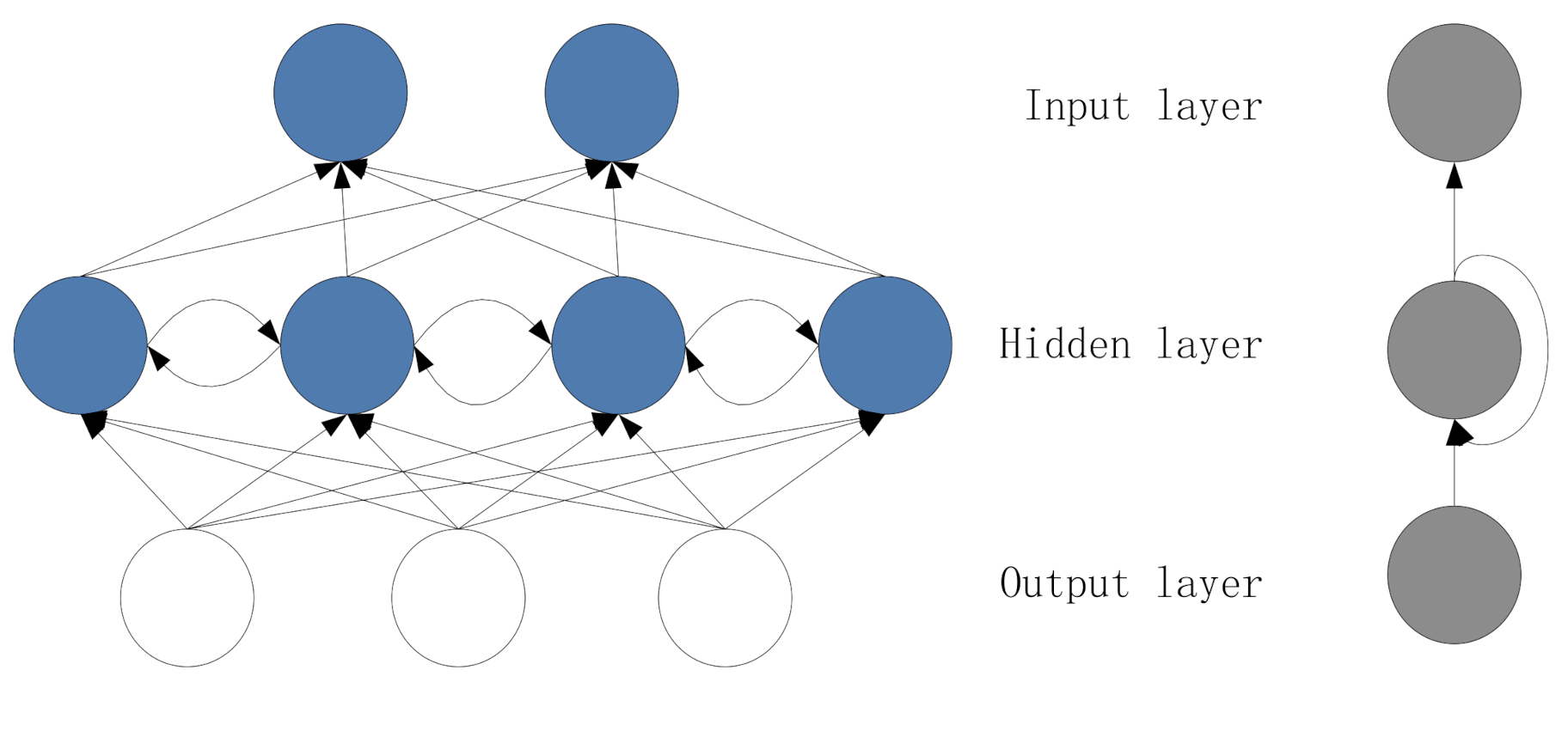
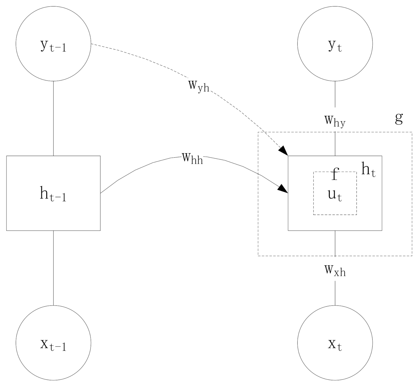
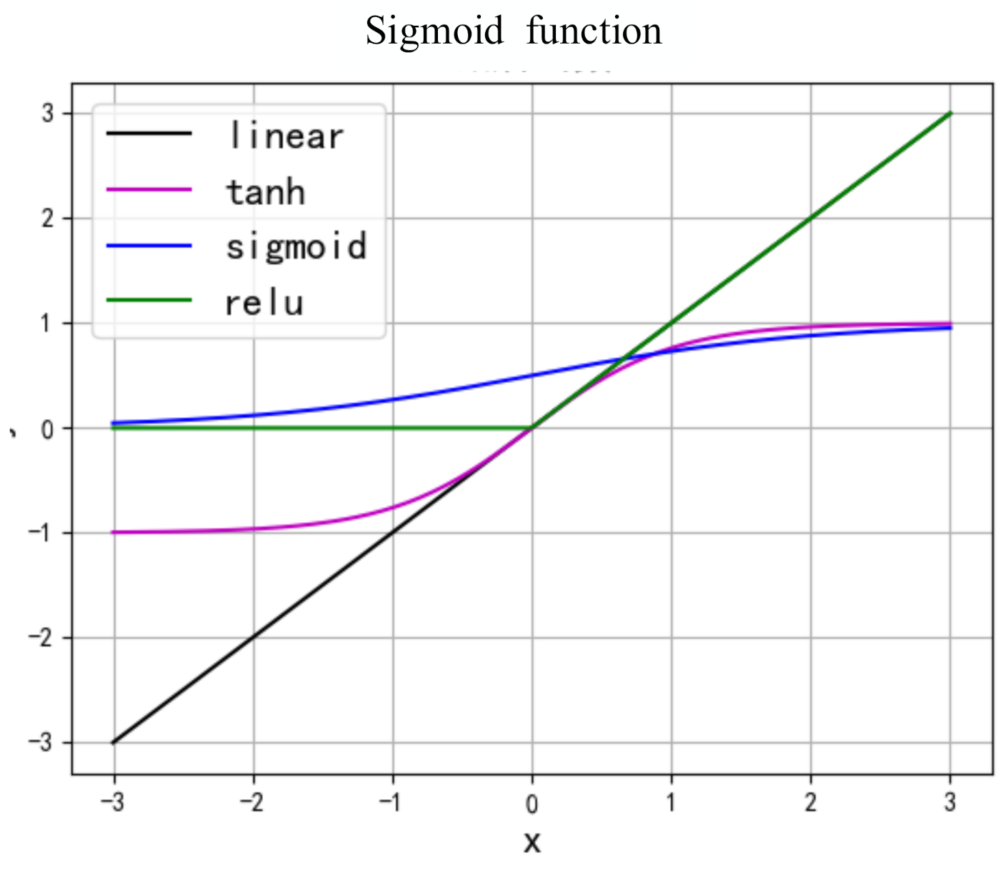
2.1. The Information of the Hidden Layer of the Recurrent Neural Network

The operational principle of the RNN relies on two things: the hidden layer and the output layer. Figure 2 shows the schematic diagram of the RNN forward propagation. where t and t − 1 are moments, W_xh is the weight matrix from the input layer to the hidden layer, W_hh is the weight matrix from the hidden layer to the hidden layer, W_hy is the weight matrix from the hidden layer to the output layer, x is the input layer information, and h is the hidden layer. y is the output layer information, f is the hidden layer activation function, and g is the output layer activation function. Generally, the hidden layer activation function uses the tanh function or rectified linear units; the output layer activation function has a linear function and a softmax function; each activation function is shown in Figure 3.

The output information of the hidden layer consists of two parts: the output information of the hidden layer at the previous moment and the output information of the input layer at the current moment.

The input information of the input layer is:

$$h_1=W_{xh}{x}_t$$

(1)

The output information of the hidden layer at the previous moment is:

$$h_2=W_{hh}{h}_{t-1}$$

(2)

The output information of the hidden layer is the sum of h₁ and h₂:

$$\begin{gathered} h_t=f\left(h_1+h_2\right) \\ =f\left(W_{xh}{x}_t+W_{hh}{h}_{t-1}\right) \end{gathered}$$

(3)

h₂ is the influence of information of the hidden layer at the previous moment on the current moment, indicating the information content that can be memorized, and $u_t=W_{xh}{x}_t+W_{hh}{h}_{t-1}$ is the N × 1 hidden layer’s latent vector.

In addition, the output at the previous moment is sometimes used to update the state at the next moment. At this time, the state variable is:

$$h_t=f\left(W_{xh}{x}_t+W_{hh}{h}_{t-1}+W_{yh}{y}_{t-1}\right)$$

(4)

2.2. Calculation of The information of the Output Layer of the Recurrent Neural Network

The information taken from the hidden layer to the output layer can be expressed as y_t. The output information h_t of the hidden layer can be derived from Equation (3). Suppose the input layer contains K neurons, the hidden layer contains N neurons, and the output layer contains L neurons. Then, the weight matrix W_xh from the input layer to the hidden layer is a K × N order matrix, the weight matrix W_hh from the hidden layer to the hidden layer is an N × N order matrix, and the weight matrix W_hy from the hidden layer to the output layer is an N × L order matrix. Then, the output of the hidden layer is:

$$v_t=W_{hy}{h}_t$$

(5)

The output information of the output layer is:

$$\begin{gathered} y_t=g\left(v_t\right) \\ =g\left(W_{hy}{h}_t\right) \end{gathered}$$

(6)

where $W_{hy}{h}_t+h_t$ is the latent vector of the L × 1 output layer.

Combining all of the above information, the output information of the output layer is:

$$y_t=g\left(W_{hy}f\left(W_{xh}{x}_t+W_{hh}{h}_{t-1}\right)\right)$$

(7)

2.3. The Backpropagation of Circulating Nerves over Time

Back propagation through time (BPTT) is used calculate the error between the inputs and outputs of neurons. Through the backpropagation of the network error and the regression of each layer, one can minimize the loss function, reach the optimization goal, and adjust the weights and thresholds of the neural units of each layer. The cyclic neural network studied in this paper is a regression task, and the square error is used as the loss function of the cyclic neural network:

$$E=c{\displaystyle \sum }_{t=1}^T\parallel I_t-y_t\parallel {}^2=c{\displaystyle \sum }_{t=1}^T{\displaystyle \sum }_{j=1}^L{(l_t\left(j\right)-y_t\left(j\right))}^2$$

(8)

where E is the loss function using the square error, y_t is the true value, and it is the predicted value. To facilitate the subsequent derivative calculation of the paper, the value of c is 0.5.

In the training process, the gradient descent method is used to determine the structural parameters of the neural network, and the loss function is minimized as the optimization goal. Equation (9) presents the weight update principle:

$$w^{new}=w-\gamma \frac{\partial E}{\partial w}$$

(9)

where $\gamma$ is the learning efficiency.

To calculate the descent gradient, the following network error terms are defined in Equation (10):

$$\begin{gathered} {\delta }_t^y\left(j\right)=-\frac{\partial E}{\partial v_t\left(j\right)} \\ {\delta }_t^h\left(j\right)=-\frac{\partial E}{\partial u_t\left(j\right)} \end{gathered}$$

(10)

where ${\delta }_t^y\left(j\right)$ is the output neuron’s error, and ${\delta }_t^h\left(j\right)$ is the hidden neuron error.

For the last time frame (T), the error of the hidden layer is:

$$\begin{gathered} {\delta }_T^h\left(j\right)=-\left({\displaystyle \sum }_{i=1}^L\frac{\partial E}{\partial v_T\left(i\right)}\frac{\partial v_T\left(i\right)}{\partial h_T\left(j\right)}\frac{\partial h_T\left(j\right)}{\partial u_T\left(j\right)}\right)={\displaystyle \sum }_{i=1}^L{\delta }_T^y\left(i\right)w_{hy}\left(i,j\right)f^{\prime }\left(u_T\left(j\right)\right) \\ for\mathrm{j}=1,2,\dots \mathrm{N} \end{gathered}$$

(11)

After matrixing:

$${\delta }_T^h=W_{hy}^T{\delta }_T^y•f^{\prime }\left(u_T\right)$$

(12)

Here, the chain rule is used to derive the error function, and the v_t calculated in the previous step can be directly applied to the calculation of the subsequent error term until the partial derivative of u_t is calculated.

The error term for other time frames is:

$$\begin{gathered} {\delta }_t^y\left(j\right)=\left(l_t\left(j\right)-y_t\left(j\right)\right)g^{\prime }\left(v_t\left(j\right)\right) \\ for\mathrm{j}=1,2,\dots ,\mathrm{L} \end{gathered}$$

(13)

After matrixing:

$${\delta }_t^y=\left(I_t-y_t\right)•g^{\prime }\left(v_t\right)$$

(14)

The error term for the recursive calculation of output nodes and hidden layer nodes is:

$$\begin{gathered} {\delta }_t^h\left(j\right)=\left[{\displaystyle \sum }_{i=1}^N{\delta }_{t+1}^h\left(i\right)w_{hh}\left(i,j\right)+{\displaystyle \sum }_{i=1}^L{\delta }_t^y\left(i\right)w_{hy}\left(i,j\right)\right]f^{\prime }\left(u_t\left(j\right)\right) \\ for j=1,2,\dots ,N \end{gathered}$$

(15)

After matrixing:

$${\delta }_t^h=\left[W_{hh}^T{\delta }_{t+1}^h+W_{hy}^T{\delta }_t^y\right]•f^{\prime }\left(u_t\right)$$

(16)

The error term ${\delta }_t^y$ is obtained from the backpropagation of the output layer in time frame t, and ${\delta }_{t+1}^h$ is the result of the backpropagation of the hidden layer in time frame t + 1. It should be noted that in contrast to time T, the intermediate time contains two parts of the backward error of backpropagation. For the last item at time T, there is no subsequent neuron, so there is only one reverse error term, y. As such, the T moment is a special moment.

2.4. Weight Updating for Reverse Broadcasting over Time

According to the weight update principle, Equation (9) can be used to obtain the updated status of the weight of each layer.

Output layer:

$$\begin{gathered} w_{hy}^{new}\left(i,j\right)=w_{hy}\left(i,j\right)-\gamma {\displaystyle \sum }_{t=1}^T\frac{\partial E}{\partial v_t\left(i\right)}\frac{\partial v_t\left(i\right)}{\partial w_{hy}\left(i,j\right)} \\ =w_{hy}\left(i,j\right)-\gamma {\displaystyle \sum }_{t=1}^T{\delta }_t^y\left(i\right)h_t\left(j\right) \end{gathered}$$

(17)

After matrixing:

$$W_{hy}^{new}=W_{hy}+\gamma {\displaystyle \sum }_{t=1}^T{\delta }_y^t{h}_t^T$$

(18)

Input layer:

$$\begin{gathered} w_{xh}^{new}\left(i,j\right)=w_{xh}\left(i,j\right)-\gamma {\displaystyle \sum }_{t=1}^T\frac{\partial E}{\partial u_t\left(i\right)}\frac{\partial u_t\left(i\right)}{\partial w_{xh}\left(i,j\right)} \\ =w_{xh}\left(i,j\right)-\gamma {\displaystyle \sum }_{t=1}^T{\delta }_t^h\left(i\right)x_t\left(j\right) \end{gathered}$$

(19)

After matrixing:

$$W_{xh}^{new}=W_{xh}+\gamma {\displaystyle \sum }_{t=1}^T{\delta }_h^t{x}_t^T$$

(20)

Hidden layer:

$$\begin{gathered} w_{hh}^{new}\left(i,j\right)=w_{hh}\left(i,j\right)-\gamma {\displaystyle \sum }_{t=1}^T\frac{\partial E}{\partial u_t\left(i\right)}\frac{\partial u_t\left(i\right)}{\partial w_{hh}\left(i,j\right)} \\ =w_{hh}\left(i,j\right)-\gamma {\displaystyle \sum }_{t=1}^T{\delta }_t^h\left(i\right)h_{t-1}\left(j\right) \end{gathered}$$

(21)

After matrixing:

$$W_{hh}^{new}=W_{hh}+\gamma {\displaystyle \sum }_{t=1}^T{\delta }_h^t{h}_{t-1}^T$$

(22)

The pseudo-code of RNN backpropagation is shown in Algorithm 1.

Algorithm 1. The time back propagation algorithm of a single-layer RNN with a square sum error function

1: procedure BPTT({xt, It}$1\le t\le T$ )

2: $\mathrm{for}t\leftarrow 1;t\le T;t\leftarrow t+1$do

3: $u_t\leftarrow W_{xh}{x}_t+W_{hh}{h}_{t-1}$

4: $h_t\leftarrow f\left(u_t\right)$

5: $v_t\leftarrow W_{hy}{h}_t$

6: $y_t\leftarrow g\left(v_t\right)$

7:      end for

8:   ${\delta }_T^y\leftarrow \left(I_T-y_T\right)•g^{\prime }\left(v_T\right)$

9:   ${\delta }_T^h\leftarrow W_{hy}^T{\delta }_T^y•f^{\prime }\left(u_T\right)$

10:   $\mathrm{for}t\leftarrow T-1;t\ge 1T;t\leftarrow t-1$do

11:         ${\delta }_t^y\leftarrow \left(I_t-y_t\right)•g^{\prime }\left(v_t\right)$

12:         ${\delta }_t^h\leftarrow \left[W_{hh}^T{\delta }_{t+1}^h+W_{hy}^T{\delta }_t^y\right]•f^{\prime }\left(u_t\right)$

13:     end for

14:     $W_{hy}\leftarrow W_{hy}+\gamma {{\displaystyle \sum }}_{t=1}^T{\delta }_y^t{h}_t^T$

15:     $W_{hh}\leftarrow W_{hh}+\gamma {{\displaystyle \sum }}_{t=1}^T{\delta }_h^t{h}_{t-1}^T$

16: end procedure

3. Experiment and Results

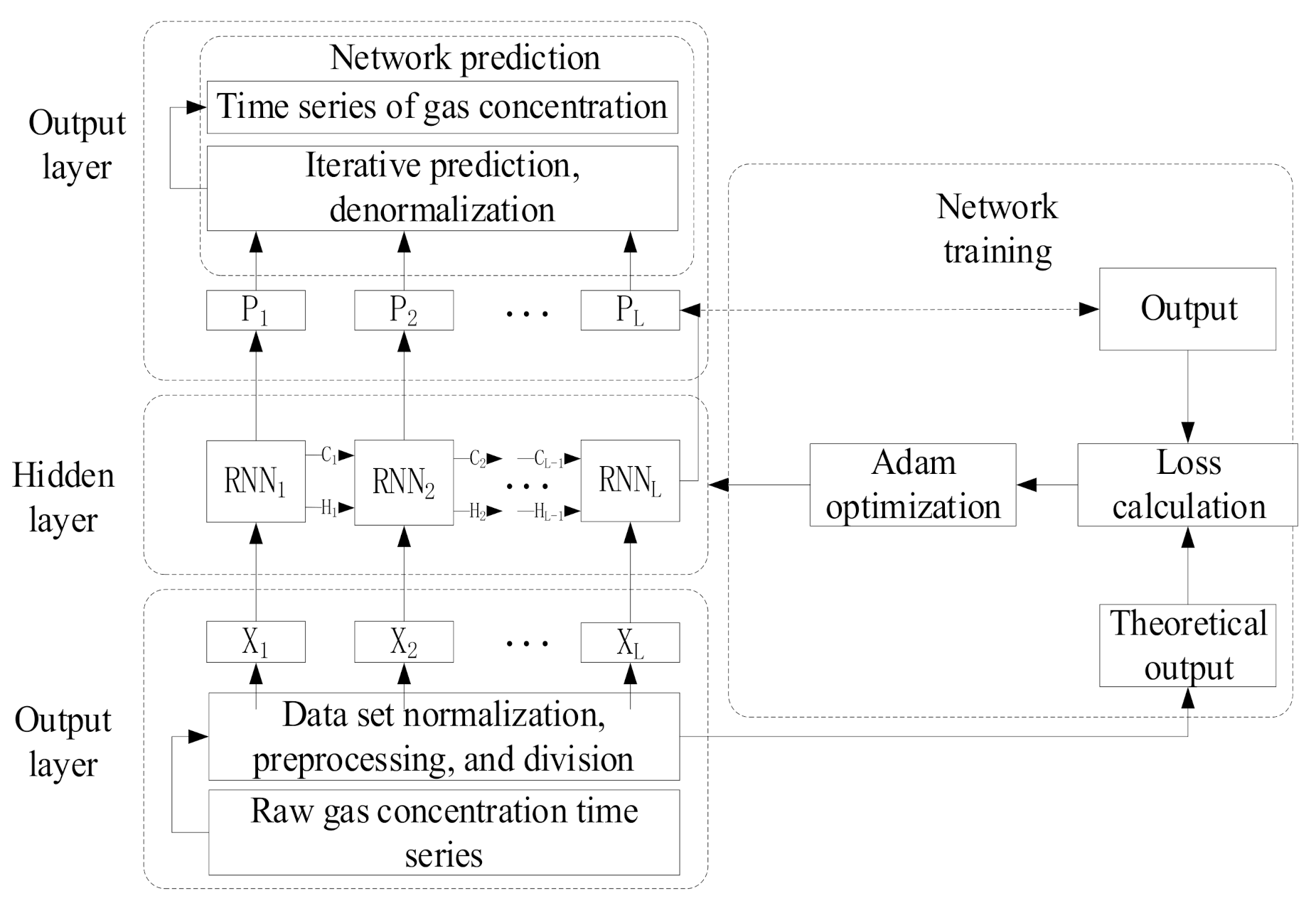
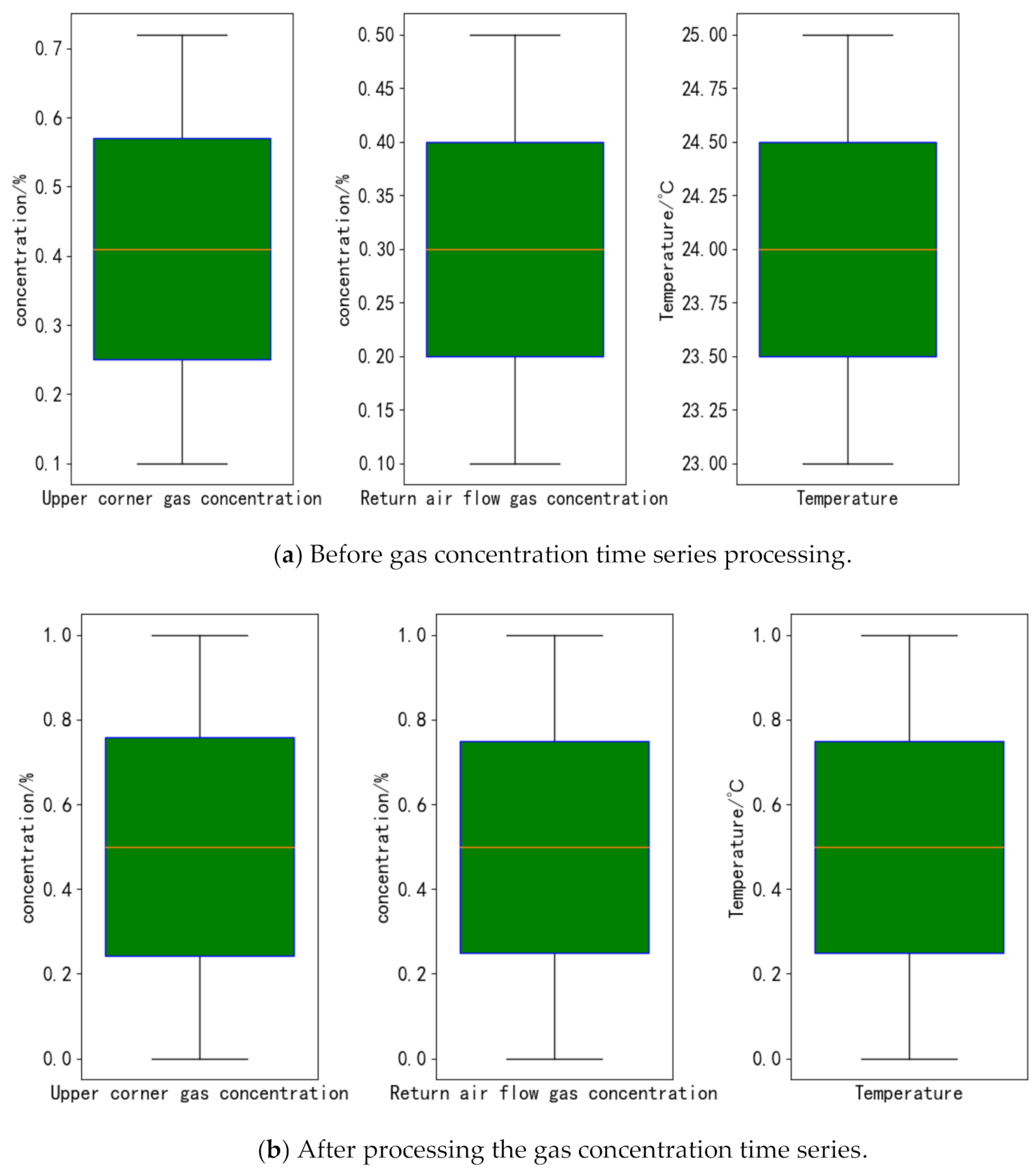
3.1. Construction of a Predictive Model

To combine the characteristics of the gas concentration time series and the advantages of RNN processed time series, the Adam optimization algorithm is used to optimize the solution process, and the RNN-based gas concentration prediction algorithm for the working face is constructed. The RNN face gas concentration prediction can be divided into three parts: data processing, network training, and network prediction. The RNN gas concentration prediction process is shown in Figure 4. The data processing processes include data cleaning, feature extraction, data partitioning, and data normalization. The network training process take the loss function minimization as the optimization goal and adopts adaptive moment estimation (Adam) optimization. For network prediction, the trained RNN prediction algorithm predicts the gas concentration time series.

The main research object of the hidden layer is network training. First, we define the gas concentration time series $F_o=\left\{f_1,f_2,\dots ,f_n\right\}$ in the network input layer; $f_i=\left\{x_{2i},x_{5i},x_{7i},x_{0i}\right\},i<n$ is the gas concentration time series after Lasso feature selection, where in the divided training set is $F_{train}=\left\{f_1,f_2,\dots ,f_m\right\}$, the test set is $F_{test}=\left\{f_{m+1},f_{m+2},\dots ,f_n\right\}$, and the relationship between m and n is m<n, m,n∈N. The MinMaxScaler method (denoted as min–max) is used to normalize $f_i$, and the normalized training set is:

$$F_{train}^{’}=\left\{f_1^{’},f_2^{’},\dots ,f_m^{’}\right\}$$

(23)

To unify the input format of the hidden layer in the network, the data are divided into $F_{train}^{’}$, and the length of the divided window is set to $L$. Then, the output of the divided model is:

$$X=\left\{X_1,X_2,\dots X_L\right\}$$

(24)

$$X_p=\left\{f_p^{’},f_{p+1}^{’},\dots ,f_{m-L+p-1}^{’}\right\}$$

(25)

$$f_p^{’}=\left\{x_{2p},x_{5p},x_{7p}\right\}$$

(26)

$$1\le p\le L;p,L\in N$$

(27)

The corresponding theoretical output is:

$$Y=\left\{Y_1,Y_2,\dots Y_L\right\}$$

(28)

$$Y_p=\left\{x_{0\left(p+1\right)}^{’},x_{0\left(p+2\right)}^{’},\dots ,x_{0\left(m-L+p\right)}^{’}\right\}$$

(29)

The output, X, is sent to the hidden layer. It can be seen from Figure 4 that the hidden layer contains L RNN units linked before and after time. After the hidden layer is calculated, X can be expressed as:

$$P=\left\{P_1,P_2,\dots P_L\right\}$$

(30)

$$P_p=RN{N}_{forward}\left(X_p,C_{p-1},H_{p-1}\right)$$

(31)

Among them, $C_{p-1}$ and $H_{p-1}$ represent the state and output of the previous RNN unit, respectively; $RN{N}_{forward}$ is t Equations (1)–(7). We set the unit state vector size to $S_{state}$; then, the size of both $C_{p-1}$ and $H_{p-1}$ is $S_{state}$. Therefore, the dimensions of hidden layer output $P$ and theoretical output $Y$ are (m − L, L, 1), which is a three-dimensional array. In addition, the loss function used in this experiment is the mean square error:

$$loss={\displaystyle \sum }_{i=1}^{L\left(m-L\right)}{(p_i-y_i)}^2/\left[L\left(m-L\right)\right]$$

(32)

Taking the minimum loss function as the optimization principle, the Adam optimization algorithm is used to update the network weights, and finally the optimal hidden layer network is obtained.

Adam (a method for stochastic optimization) is a first-order optimization algorithm. Compared with the traditional gradient descent algorithm, the optimization performance has been greatly improved. Based on the training sample data, the network is continuously iterated to update the weight and threshold of the neural network. Adam combines the superior performance of AdaGrad and RMSProp algorithms, and can solve most of the sparse gradient and noise problems by setting parameters. The parameters in the Keras framework are lr = 0.001, ${\beta }_1$ = 0.9, ${\beta }_2$= 0.999, and $\epsilon =le^08$; lr is the learning efficiency; ${\beta }_1$ and ${\beta }_2$ are the exponential decay rates of the moment estimation; $\epsilon$ is a very small number to prevent division by zero in the calculation; the initial value of both $m_t$ and $v_t$ is 0. The algorithm update method is as follows:

First-order moment estimation and second-order moment estimation:

$$m_t={\beta }_1\ast m_{\mathrm{t}-1}+\left(1-{\beta }_1\right){\ast \mathrm{g}}_t$$

(33)

$$v_t={\beta }_2\ast v_{\mathrm{t}-1}+\left(1-{\beta }_2\right){\ast \mathrm{g}}_t\text{^}2$$

(34)

First-order moment estimation deviation correction and second-order moment estimation deviation correction:

$${m^{\prime }}_t=\frac{m_t}{\left(1-{\beta }_1^t\right)}$$

(35)

$${v^{\prime }}_t=\frac{v_t}{\left(1-{\beta }_2^t\right)}$$

(36)

Parameter update:

$${\theta }_t={\theta }_{t-1}-\alpha \ast \frac{{m^{\prime }}_t}{\left(\sqrt{{v^{\prime }}_t}+\epsilon \right)}$$

(37)

3.2. Experimental Verification of Multi-Parameter Fusion Prediction Model of Pressure Relief Gas Concentration Based on RNN

This experiment used coal mine production monitoring data from 1 July to 2 November 2018 as the training sample, a total of 10,000 pieces of data, based on the gas concentration time series data. This experiment used the cubic exponential smoothing method to impute missing items in the data. The approximate mean method was used to replace outliers in the data. The MinMaxScaler method was used to normalize the data, and the Lasso method was used to perform feature selection on the data samples. It uses a 7:3 data set division and divides the processed data into a training set and a test set. The training set was used to train the prediction model. The test set was used to test the learning effect of the predictive model. Therefore, the training set had 7000 pieces of data, and the test set had 3000 pieces of data. There were three characteristic variables related to the gas concentration in the working face, the gas concentration in the upper corner, the gas concentration in the return air flow, and the temperature. A detailed view of the time series of gas concentration is shown in Figure 5.

To ensure the performance of the prediction model, two evaluation indicators, mean square error (MSE) and running time, were used to evaluate the performances of the following trained RNN prediction models. The prediction model’s operating principle is shown in Equation (38):

$$MSE=\frac{1}{n}{\displaystyle \sum }_{i=1}^n{(f_i-y_i)}^2$$

(38)

where f_i is the predicted value of the gas concentration; y_i is the true value of the gas concentration.

In addition, the computer configuration used in this experiment was as follows: the processor was CPU (i7-8700), the speed was 3.2 GHz/3.19 GHz, the memory was 32.00 GB, the operating system was Windows10 (64-bit), and the programming language was python3. 6.5—integrated development environment PyCharm Community Edition 2017.2.3. In the program design process, the RNN, SVR, and BP neural network were implemented by Keras 2.2.4 and scikit-learn 0.19.1 program packages.

4. Discussion

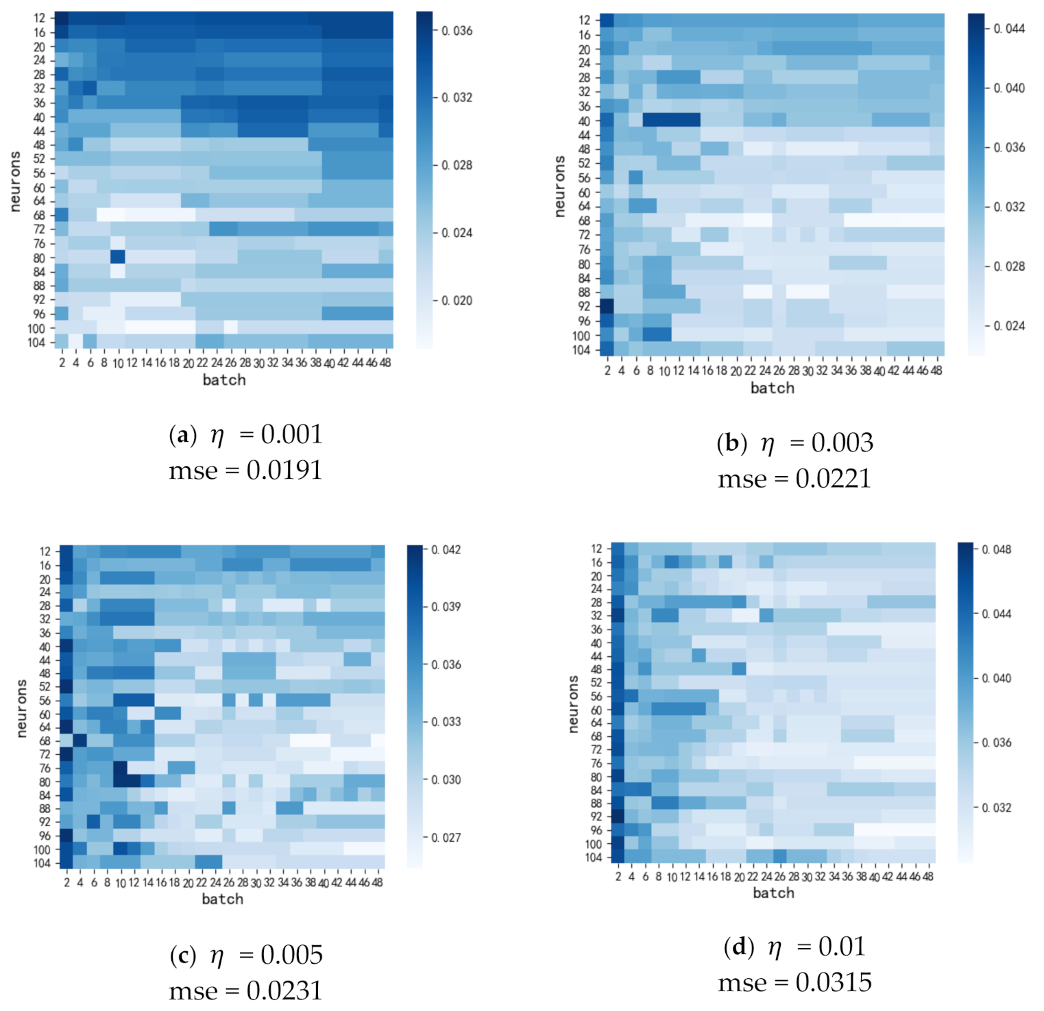
4.1. Comparison of the Hyperparameter Tuning of Learning Rate, Batch Size, and Neuron

(1) Setting the hyperparameters

According to Algorithm 2. this experiment first fixed the values of non-key parameters—random seed, seed = 2, and 100 training steps—and then set the value ranges of three parameters—batch size {2, 4,…48}, number of neurons {12, 16,…104}, and the learning rate {0.001, 0.003, 0.005, 0.01}—and finally set the objective function to the minimum MSE.

Algorithm 2. the training and prediction of a gas concentration prediction model for a working face based on the RNN.

Input: $F_o,m,L,S_{state},seed,steps,\eta$

1.  get $F_{train}$,$F_{test}$ from $F_o$ by m

2.  $F_{train}^{’}$= min-max($F_{train}$)

3.  get $X$,$Y$ from $F_{train}^{’}$ by L

4.  create $RN{N}_{cell}$ by $S_{state}$

5.  connect $RN{N}_{net}$ by $RN{N}_{cell}$ and L

6.  connect $RN{N}_{net}$ by seed

7.  for each step in 1: steps

8.      $P$ =$RN{N}_{forward}\left(X\right)$

9.       $loss={{\displaystyle \sum }}_{i=1}^{L\left(m-L\right)}{(p_i-y_i)}^2/\left[L\left(m-L\right)\right]$

10.       update $RN{N}_{net}$ by Adam with loss and $\eta$

11.   get $RN{N}_{net}^{\ast }$

12.   for each j in 0: (n-m-1)

13.        $P_{f+j}=RN{N}_{net}^{\ast }\left(Y_{f+j}\right)$

14.        append $P_0$ with $P_{f+j}$ [−1]

15.   $P_{te}=de\_\min -\max (P_o)$

16.   error measure $\epsilon \left(P_{test},F_{test}\right)$,${\epsilon }_e\left(P_{train},F_{train}\right)$

The batch size represents the maximum number of samples for each model’s training. As the batch size increases, the convergence speeds up; however, it is easy to miss the optimal solution; the number of neurons represents the learning ability of the model, and the expression ability of the model increases as the number of neurons increases. However, the operating cost will also see a corresponding increase while increasing the probability of overfitting.

The RNN model training process mainly involves the input layer, hidden layer, output layer, and network training part. The prediction process mainly involves the output layer. ${\mathrm{RNN}}_{\mathrm{net}}$ means the hidden layer network of the RNN model, ${\mathrm{RNN}}_{\mathrm{cell}}$ means the neural unit in the hidden layer of the RNN model, and $\mathsf{\epsilon }$ means the error measurement function.

(2) Analysis of experimental results

Figure 6 shows the training results of using the grid search method to optimize RNN hyperparameters. The independent variable in each sub-graph is batch size, and the dependent variable is the number of neurons. Different sub-graphs correspond to different values. Mse is the minimum MSE in the sub-graph. The lighter the color of a square in the grid, the smaller the MSE. Figure 6 shows that with an increase in batch size, the MSE became larger. When = 0.001, the MSE could converge to the lowest range; at the same time, the batch size value range was [10,20], and the neuron value was 68. It was easy to obtain a higher accuracy, and the minimum MSE was 0.0191.

(3) Experimental results

The top five optimal parameter combinations of the RNN model and the corresponding model accuracy are shown in

Table 1. Number of batches and neurons, and training performance.

Rank	Model Parameters			MSE	Time/s
	Batch	Neurons	$\mathit{\eta }$
1	10	68	0.001	0.0191	421
2	12	100	0.001	0.0192	601
3	34	68	0.003	0.0219	312
4	20	68	0.003	0.0221	352
5	10	104	0.001	0.0222	782

.

It can be seen that it was easier to obtain higher accuracy when $\eta$ was 0.001. When the number of batches was 10 and the number of neurons was 68, the model’s prediction accuracy was the best. The experimental results show that, for $\eta$, the smaller the value, the higher the prediction accuracy. At the same time, selecting reasonable values for the numbers of batches and neurons can effectively avoid over-fitting problems, increase the learning ability of the model, and improve the prediction accuracy of the model.

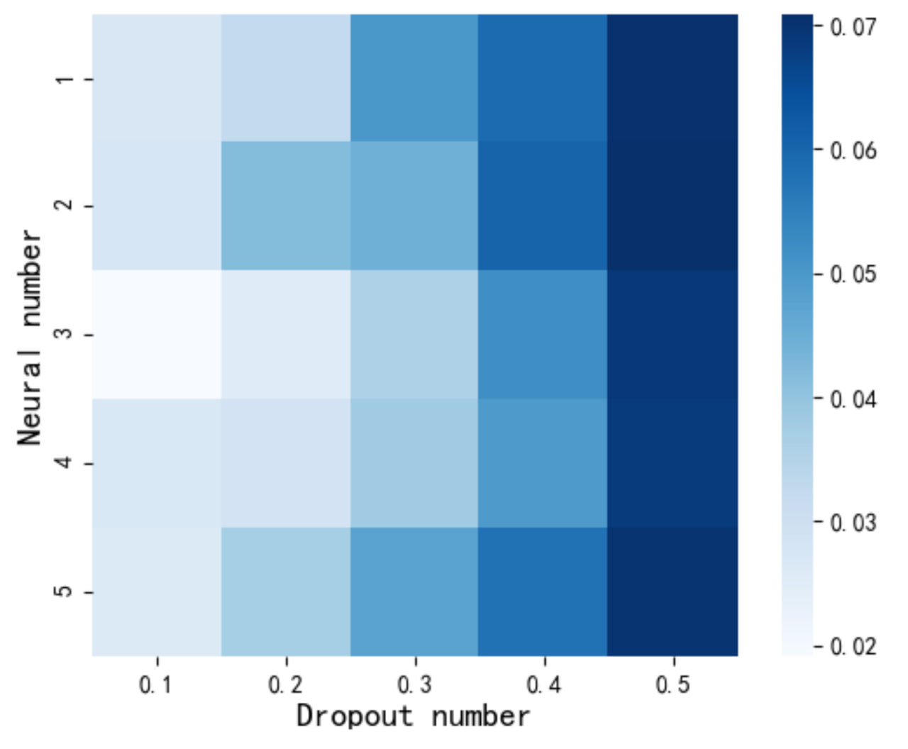
4.2. Hyperparameter Tuning Comparison of Network Depth and Discard Ratio

(1) Hyperparameter setting

According to the training results, this experiment first fixed the parameter values: random seed, seed = 2, 100 training steps, 10 batches, 68 hidden layer neurons, learning rate $\eta$ = 0.001. Then, it set two parameters: the value ranges of the dropout ratio, Dropout $\in$ {0.1, 0.2, 0.3, 0.4, 0.5}, and network depth $\in$ {1, 2, 3, 4, 5}; finally, it set the objective function to be the minimum MSE.

Dropout represents the proportion of randomly inactivated neurons in the prevention of overfitting. A decrease in the proportion will increase the capacity of the model. Fewer dropped parameters means that the adaptability between model parameters and the capacity between models will increase, but this will not necessarily increase the model’s accuracy. When the discarding ratio is too large, the model parameters will be reduced, thereby reducing the ability of the model to learn and express; an increase in the network depth of the model means an increase in the model capacity; under the same conditions, an increase in the network depth means more parameters and a stronger fitting ability; as the network depth increases, the model becomes increasingly complex, and it is increasingly likely to cause over-fitting.

(2) Analysis of experimental results

Figure 7 shows the training results of using the grid search method to optimize the RNN hyperparameters. As the discarding ratio increased, the model’s ability to prevent overfitting became stronger; however, the problem of underfitting became increasingly serious. As shown in Figure 7, as the discarding ratio increased from 0.1 to 0.5, the model’s error became larger (see the darker colors in the figure); in addition, as the network depth increased, the parameters increased increasingly in number, and the model learned and showed capability when the number of parameters was increased to a certain extent. Although the model’s learning and predictive abilities were very strong, the complexity of the model increased gradually, which caused a higher probability of overfitting, leading to higher errors and model depth. When it had 1 to 3 layers, the model’s error gradually decreased (see the lighter colors in the figure), and when the model’s depth increased to five layers, the predictions started to improve (see the darker colors in the figure). In addition, the experiment found that the smaller the model’s discarding ratio, the smaller the training error; as the network depth increased, the model’s training error showed a parabolic trend, and the error first increased and then decreased.

(3) Experimental results

The detailed performance in terms of the dropout ratio and network depth for the RNN gas concentration prediction method is shown in

Table 2. Dropout ratio and network depth performance.

Rank	Model Parameters		Performance
	Dropout Ratio	Layers	MSE	Time/s
1	0.1	3	0.0191	600
2	0.2	3	0.0255	631
3	0.1	4	0.0261	871
4	0.1	2	0.0271	125
5	0.1	1	0.0277	57

.

From the table, the model’s parameter discarding ratio was 0.1, and when the network depth was three layers, the minimum model error was 0.0191. In addition, when the discarding ratio was 0.1, the probability of obtaining a lower error was higher.

Based on the optimization results of the previous two sections, this experiment first fixed the values of the key parameters: random seed, seed = 2, 100 training steps, 10 batches, 68 hidden layer neurons, learning rate 0.001, and dropout ratio 0.1. The network depth was three layers, and finally the objective function was set to the highest prediction accuracy (minimum MSE) at the test point, and the early stopping method was used to find the best training times. The training effect of the early stopping method is shown in Figure 8.

This experiment used the early stopping method for training, while monitoring the error of the validation set. When the error in the validation set increased continuously for five training times, the training was stopped, and the weight parameter in the previous iteration result was used to the model the final parameters. As shown in Figure 8, when the number of training epochs was 80, the validation set’s error was 0.0195, and the error continued to increase during five consecutive trainings; the validation set error was 0.0201. The experiment found that after 85 training epochs, the RNN prediction model appeared to be over-fitting, and the error of the training set continued to decrease, but the corresponding validation set error gradually increased, and the validation set error oscillated. According to the principle of the early stopping method, this experiment will train the sample 80 times.

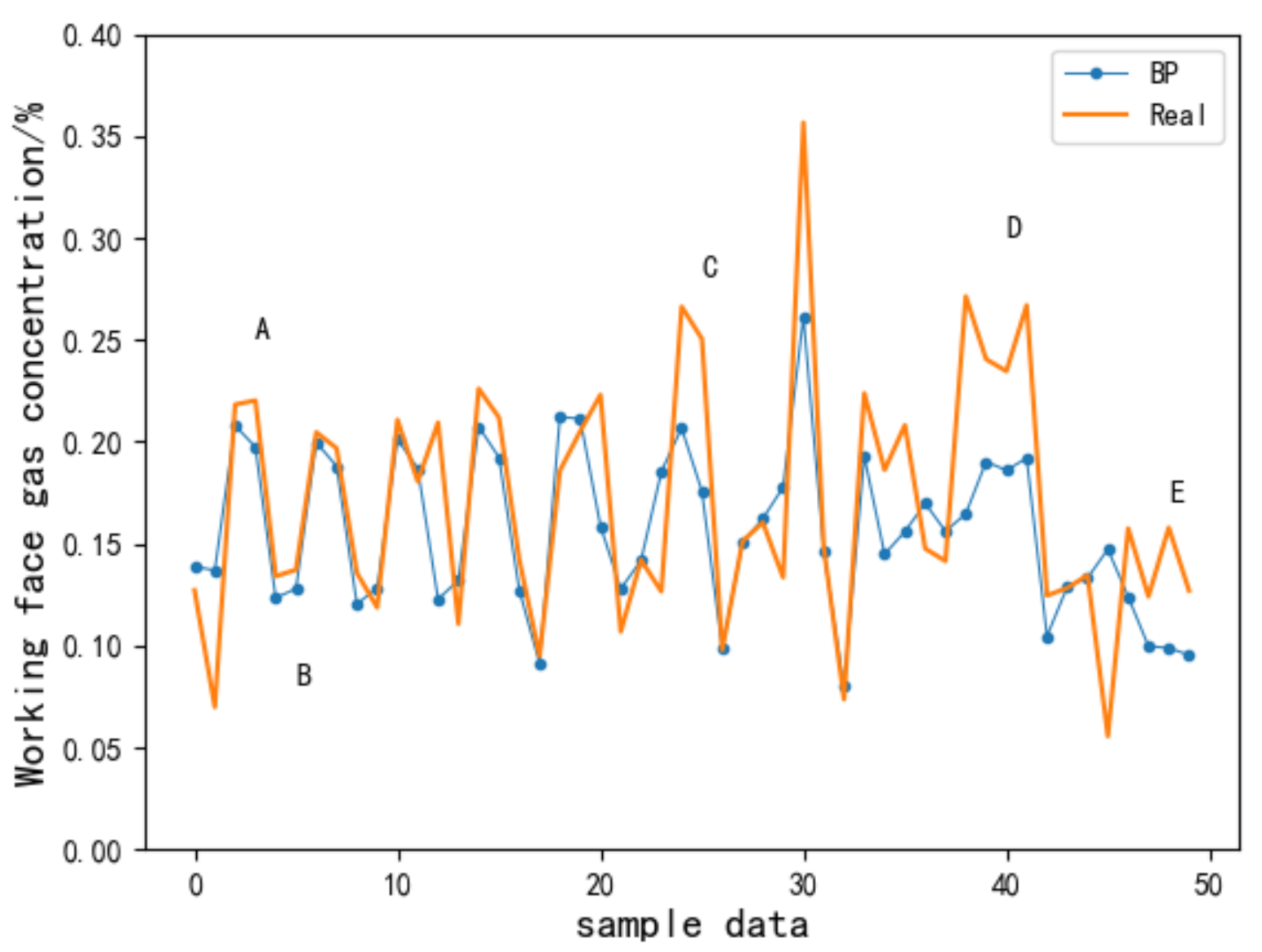
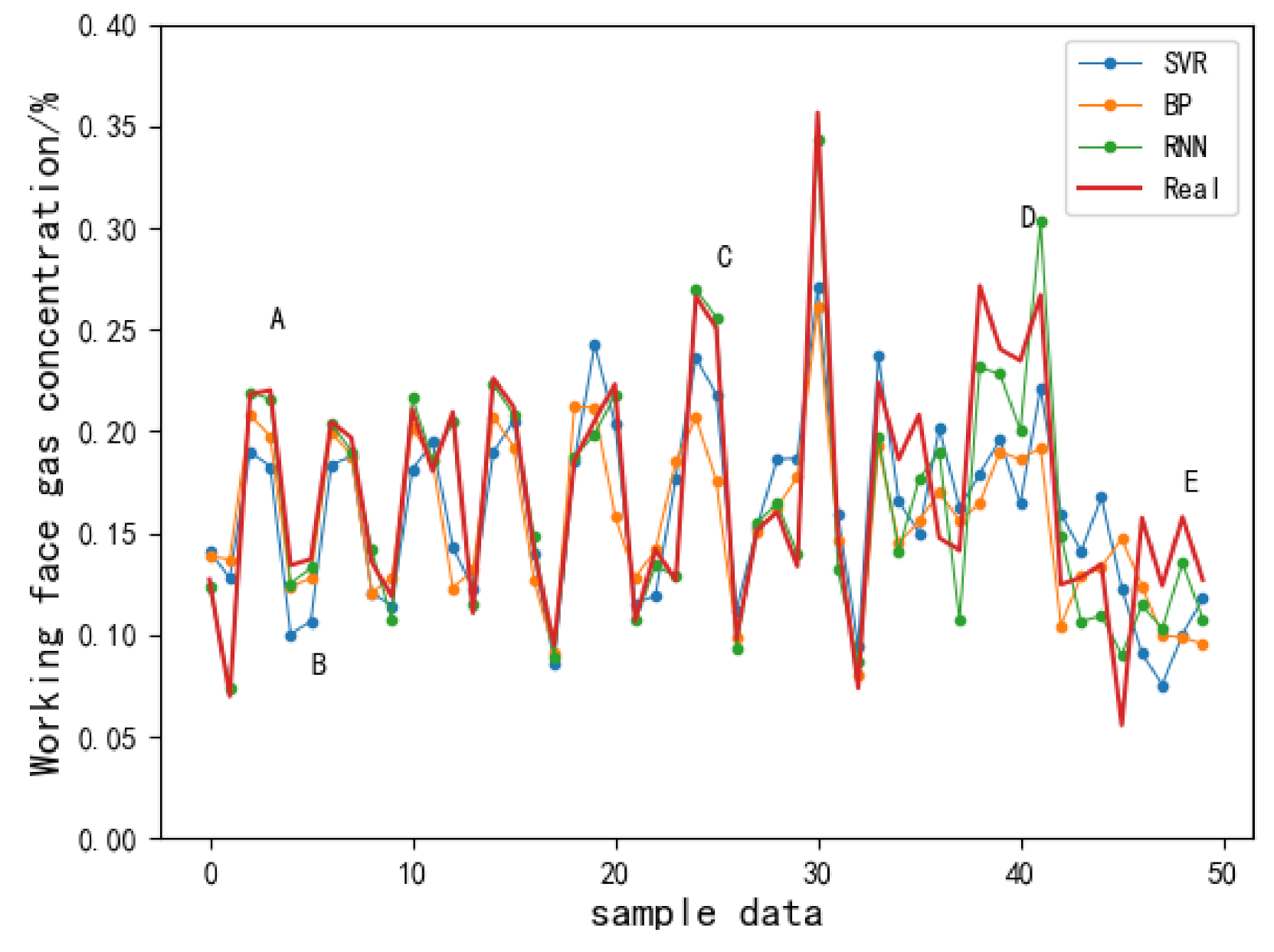
4.3. Comparison of Prediction Performances of Different Models

To ensure the prediction performance of the prediction model, the average absolute percentage error (MAPE) evaluation index was used to evaluate the prediction performance of the three optimized prediction algorithms (SVR, BP, and RNN). This operation is shown in Equation (39):

$$MAPE=\frac{1}{n}{\displaystyle \sum }_{i=1}^n\left|\frac{f_i-y_i}{y_i}\right|\ast 100\%$$

(39)

where f_i is the predicted value of the gas concentration; y_i is the true value of the gas concentration.

The fitting diagram of the multi-parameter fusion prediction effect of the working face gas concentration using the SVR method is shown in Figure 9. Based on the figure, the SVR method could learn the changing trend of the gas concentration time series, and could roughly fit the changing trend of the gas concentration. However, as the prediction length increased, the prediction error of the SVR prediction method gradually increased. In particular, at the inflection points of some gas concentration changes, the prediction error was too large.

Figure 10 shows the fitting diagram of the multi-parameter fusion prediction of the coal face gas concentration using PSO-Adam-BP. The parameter set in the PSO-Adam model needs to analyze the actual optimization problem. This paper used a three-layer neural network structure. The number of hidden layer neurons was 48, the batch size was 10, the activation functions of the hidden layer and the output layer used the “tansig” and “relu” functions, a dropout layer was added to prevent overfitting, the discarding ratio was 0.1, and the number of training samples optimized by the early stopping method was 20. From the figure, the PSO-Adam-BP method could learn the changing trend of the gas concentration time series, and could essentially fit the changing trend of the gas concentration. Compared with the SVR method, the prediction performance was better, but with the increases in the length of the prediction, the prediction error of the method based on PSO-Adam-BP was gradually increased. In particular, at the time inflection points of some gas concentration transformations, the prediction error was too large.

To study the universality and popularization of the RNN method, the coal mine production monitoring data were used as the research object to compare and analyze the prediction performance of each method in other mine applications. The comparison of the prediction results of different methods is shown in Figure 11.

The SVR, BP neural network, and RNN can roughly fit the gas concentration change trend in the prediction process; however, the prediction of the RNN performed best at the time inflection points of certain concentration changes. As shown in the Figure 11, at the A~D stages, the three prediction methods could fit the changing trend of gas concentration, but at the time inflection point of certain gas concentration changes—at points A, B, C, and D in the figure—the error of the RNN was obviously smaller than the prediction errors of the SVR and BP neural network models; in addition, when the prediction length was 40–50 units, the RNN prediction method could fit the changing trend of gas concentration, but the SVR and BP neural network methods could no longer achieve adequate prediction, especially at point E in the figure; there, the prediction errors of the SVR and BP neural network methods were relatively large.

Generally speaking, the RNN had better predictions than the SVR and BP.

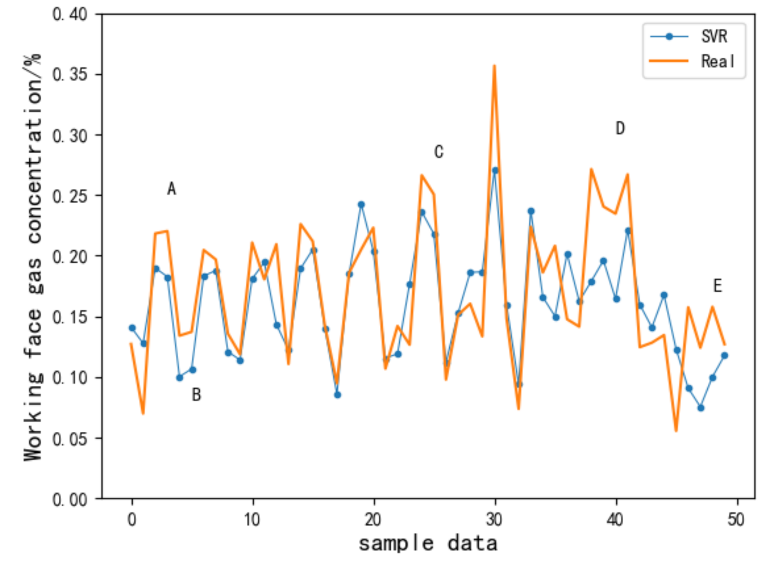
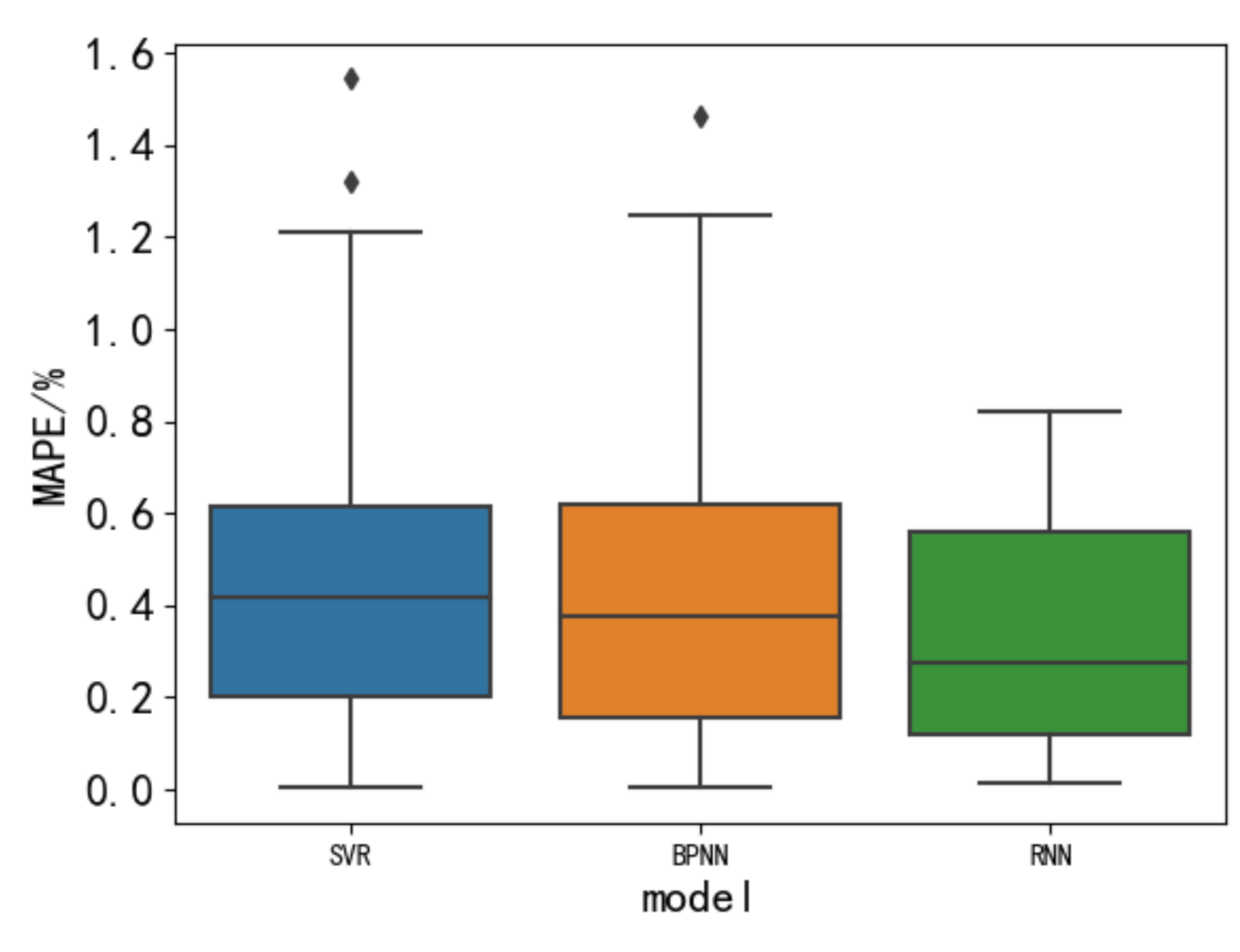
4.4. Comparative Analysis of Gas Concentration Prediction Errors Based on the SVR, BP, and RNN

The MAPEs of predictions by different methods are shown in Figure 12. The SVR and BP neural network prediction methods had many large prediction errors in the prediction process. Unlike the SVR and BP neural network prediction methods, the prediction of the BP neural network method’s MAPE was mainly concentrated between 0.19% and 0.59%.

Table 3. Comparison of prediction errors of different models.

Models	SVR	BP Neural Network	RNN
Average MAPE /%	0.4872	0.4458	0.3384
Median MAPE /%	0.4134	0.3842	0.2825

shows a detailed performance comparison of the prediction errors of different models. The experimental results showed that the average MAPEs of the SVR and BP neural network were 0.4872% and 0.4458%, respectively; the average MAPE predicted by the RNN could be reduced to 0.3384%; the median MAPE of SVR and BP neural network are 0.4134% and 0.3842%, respectively; the RNN’s median MAPE was 0.2825%.

5. Conclusions

(1)

Adam’s optimized RNN model had higher accuracy and stability than the BP neural network and SVR. During training, MAE can be reduced to 0.0573 and RMSE can be reduced to 0.0167, while MAPE can be reduced to 0.3384% during prediction.

(2)

Compared with the RNN gas concentration prediction model, SVR was more suitable for processing data samples with small data volumes and weak feature correlation. For gas concentration time series problems with large data samples and strong feature correlation, the prediction accuracy cannot meet the requirements; a BP neural network can be applied to large samples and high-dimensional samples; however, the ability to deal with data before and after the correlation is weak; compared to the BP neural network and SVR, RNN was more suitable for processing data related to time series due to its memory cell structure.

(3)

The recurrent neural network has the advantages of memory function, reasonable weight distribution, gradient descent, and backpropagation. It can memorize the current input information. When it comes to continuous, context-related tasks, it has more advantages than traditional artificial neural networks.

(4)

Compared with the RNN, although SVR and BP neural network methods could learn the transformation trend of a gas concentration time series, when it involved the inflection point of a gas concentration change associated with the front and back, the prediction performance was poor.

(5)

The RNN gas concentration prediction method and parameter optimization method based on Adam optimization can effectively predict gas concentration. Compared with the traditional BP neural network and the SVR method, the RNN method had higher accuracy and, at the same time had better robustness and applicability in terms of prediction stability. Therefore, this method has higher accuracy and could provide guidance for mine gas management.

References

- Fu, H.; Dai, W. Dynamic Prediction Method of Gas Concentration in PSR-MK-LSSVM Based on ACPSO. J. Transduct. Technol. 2016, 29, 903–908. [Google Scholar]
- Fu, H.; Yu, H.; Meng, X.Y.; Sun, L. A New Method of Mine Gas Dynamic Prediction Based on EKF-WLS-SVR and Chaotic Time Series Analysis. Chin. J. Sens. Actuators 2015, 28, 126–131. [Google Scholar]
- Fu, H.; Feng, S.C.; Liu, J.; Tang, B. The Modeling and Simulation of Gas Concentration Prediction Based on De-Eda-Svm. Chin. J. Sens. Actuators 2016, 29, 285–289. [Google Scholar]
- Liu, J.E.; Yang, X.F.; Guo, Z.L. Prediction of Coal Mine Gas Concentration Based on FIG-SVM. China Saf. Sci. J. 2013, 23, 80–84. [Google Scholar]
- Wang, Q.J.; Cheng, J.L. Forecast of coalmine gas concentration based on the immune neural network model. J. China Coal Soc. 2008, 33, 665–669. [Google Scholar]
- Liu, Y.J.; Zhao, Q.; Hao, W.L. Study of Gas Concentration Prediction Based on Genetic Algorithm and Optimizing BP Neural Network. Min. Saf. Environ. Prot. 2015, 42, 56–60. [Google Scholar]
- Fu, H.; Li, W.J.; Meng, X.Y.; Wang, G.H.; Wang, C.X. Application of IGA-DFNN for Predicting Coal Mine Gas Concentration. Chin. J. Sens. Actuators 2014, 27, 262–266. [Google Scholar]
- Yang, L.; Liu, H.; Mao, S.J.; Shi, C. Dynamic prediction of gas concentration based on multivariate distribution lag model. J. China Univ. Min. Technol. 2016, 45, 455–461. [Google Scholar]
- Wang, X.L.; Liu, J.; Lu, J.J. Gas Concentration Forecasting Approach Based on Wavelet Transform and Optimized Predictor. J. Basic Sci. Eng. 2011, 19, 499–508. [Google Scholar]
- Xiang, W.; Qian, J.S.; Huang, C.H.; Zhang, L. Short-term coalmine gas concentration prediction based on wavelet transform and extreme learning machine. Math. Probl. Eng. 2014. [Google Scholar] [CrossRef]
- Ma, X.L.; Hua, H. Gas concentration prediction based on the measured data of a coal mine rescue robot. J. Robot. 2016. [Google Scholar] [CrossRef]
- Yang, S.; Fan, B.; Xie, L.; Wang, L.J.; Song, G.P. Speech-driven video-realistic talking head synthesis using BLSTM-RNN. J. Tsinghua Univ. (Sci. Technol.) 2017, 57, 250–256. [Google Scholar]
- Li, Y.X.; Zhang, J.Q.; Pan, D.; Hu, D. A Study of Speech Recognition Based on RNN-RBM Language Model. J. Comput. Res. Dev. 2014, 51, 1936–1944. [Google Scholar]
- Xiao, A.L.; Liu, J.; Li, Y.Z.; Song, Q.W.; Ge, N. Two-Phase Rate Adaptation Strategy for Improving Real-Time Video QoE in Mobile Networks. China Commun. 2018, 15, 12–24. [Google Scholar] [CrossRef]
- Lee, D.; Lim, M.; Park, H.; Kang, Y.; Park, J.S.; Jang, G.J.; Kim, J.H. Long Short-Term Memory Recurrent Neural Network-Based Acoustic Model Using Connectionist Temporal Classification on a Large-Scale Training Corpus. Chin. Commun. 2017, 14, 23–31. [Google Scholar] [CrossRef]
- Shi, L.; Du, J.P.; Liang, M.Y. Social Network Bursty Topic Discovery Based on RNN and Topic Model. J. Commun. 2018, 39, 189–198. [Google Scholar]
- Gou, C.C.; Qin, Y.J.; Tian, T.; Wu, D.Y.; Liu, Y.; Cheng, X.Q. Social messages outbreak prediction model based on recurrent neural network. J. Softw. 2017, 28, 3030–3042. [Google Scholar]
- Li, J.; Lin, Y.F. Prediction of time series data based on multi-time scale run. Comput. Appl. Softw. 2018, 35, 33–37. [Google Scholar]
- Zhang, X.G.; Li, Y.D.; Zhang, L.; Fan, Q.F.; Li, X. Taxi travel destination prediction based on SDZ-RNN. Comput. Eng. Appl. 2018, 54, 143–149. [Google Scholar]
- Wang, X.X.; Xu, L.H. Short-term Traffic Flow Prediction Based on Deep Learning. J. Transp. Syst. Eng. Inf. Technol. 2018, 18, 81–88. [Google Scholar]
- Mehdi, P.; Arezoo, K. Optimising cure cycle of unsaturated polyester nanocomposites using directed grid search method. Polym. Polym. Compos. 2019, 27, 1–9. [Google Scholar]
- Fayed, H.A.; Atiya, A.F. Speed up grid-search for parameter selection of support vector machines. Appl. Soft Comput. 2019, 80, 80–92. [Google Scholar] [CrossRef]
- Sun, J.L.; Wu, Q.T.; Shen, D.F.; Wen, Y.J.; Liu, F.R.; Gao, Y.; Ding, J.; Zhang, J. TSLRF: Two-Stage Algorithm Based on Least Angle Regression and Random Forest in genome-wide association studies. Sci. Rep. 2019, 9, 15–26. [Google Scholar] [CrossRef] [PubMed]
- Zhang, T.J.; Song, S.; Li, S.G.; Ma, L.; Pan, S.B.; Han, L.Y. Research on Gas Concentration Prediction Models Based on LSTM Multidimensional Time Series J. Energies. 2019, 12, 1–15. [Google Scholar] [CrossRef]
- Zhao, X.G.; Song, Z.W. ADAM optimized CNN super-resolution reconstruction. Comput. Sci. Explor. 2019, 13, 858–865. [Google Scholar]
- Yang, G.C.; Yang, J.; Li, S.B.; Hu, J.J. Modified CNN algorithm based on Dropout and ADAM optimizer. J. Huazhong Univ. Sci. Technol. (Nat. Sci. Ed.) 2018, 46, 122–127. [Google Scholar]
- Wei, Y.; Mei, J.L.; Xin, P.; Guo, R.W.; Li, P.L. Application of support vector regression cooperated with modified artificial fish swarm algorithm for wind tunnel performance prediction of automotive radiators. Appl. Therm. Eng. 2020, 3, 164–188. [Google Scholar]
- Boukhalfa, G.; Belkacem, S.; Chikhi, A.; Benaggoune, S. Application of Fuzzy PID Controller Based on Genetic Algorithm and Particle Swarm Optimization in Direct Torque Control of Double Star Induction Motor. J. Cent. South Univ. 2019, 26, 1886–1896. [Google Scholar] [CrossRef]
- Wang, P.; Wu, Y.P.; Wang, S.P.; Song, C.; Wu, X.M. Study on Lagrange-ARIMA real-time prediction model of mine gas concentration. Coal Sci. Technol. 2019, 47, 141–146. [Google Scholar]