Abstract
This paper presents an advanced adaptive single-pole auto-reclosing (ASPAR) scheme based on harmonic characteristics of the secondary arc voltage. For analysis of the harmonics, short-time Fourier transform (STFT), which is a universal signal processing tool for transforming a signal from the time domain to the frequency domain, is utilized. STFT is applied to extract the abnormal harmonic signature from the voltage waveform of a faulted phase when a transient or permanent fault occurs on a power transmission line. The proposed scheme uses the total harmonic distortion (THD) factor to determine the fault type based on the variation and distortion characteristics of the harmonics. Harmonic components in the order of odd/even are also utilized to detect the secondary arc extinction time and guide the reclosing operation. Based on these factors, two coordinated algorithms are proposed to reduce the unnecessary dead time in conventional auto-reclosing methods and enable an optimal reclosing operation in the event of a single-pole to ground fault. The proposed ASPAR scheme is implemented using the electromagnetic transient program (EMTP), and various simulations are conducted for actual 345 and 765 kV Korean study systems.
1. Introduction
It has been established that the most frequent faults on overhead high-voltage transmission lines are single-pole to ground faults, which are primarily non-permanent faults. The large majority of these faults are transient faults caused by natural events, such as flashover of the insulator caused by a high transient voltage induced by lightning or temporary tree contact [1,2,3,4]. For such faults, the single-pole auto-reclosing (SPAR) method can be implemented to improve the transient stability and reduce the reclosing voltage transients [1]. Generally, transient single-pole to ground faults are accompanied by arcs that can be classified as either primary or secondary arcs. A primary arc exists before the faulted-phase circuit breaker (CB) is tripped to remove the fault from the power system after the fault event, whereas a secondary arc occurs after the faulted-phase CB is tripped. In particular, secondary arcs are sustained by the electromagnetic and electrostatic coupling between the faulted phase and the remaining two sound phases. If the SPAR operation is performed before complete extinction of the secondary arc, it can adversely affect the power system stability. For a successful SPAR from these risky arcs, it is necessary to conduct the reclosing after the occurrence of the final extinction of the secondary arc.
In general, there are two types of SPAR schemes: traditional auto-reclosing [5,6,7,8] and adaptive auto-reclosing [9,10,11,12]. The traditional methods use a constant predetermined time called the “fixed dead time” for the arc extinction, whereas the adaptive methods monitor the conditions of the power system in real-time to determine whether the secondary arc is extinct and then perform the reclosing after the secondary arc is completely eliminated. Currently, traditional auto-reclosing methods are widely used in numerous transmission systems. However, these traditional methods have three potential disadvantages. The first problem arises after the fixed dead time. If the fault still remains as a result of allowing insufficient time to deionize the arc completely, the reclosing can cause an overvoltage across the CB poles and an arc restrike. The second problem occurs when the fault is cleared much sooner than the reclosing command with a fixed dead time. In this case, the power system stability and reliability can be reduced. The third problem is the unnecessary reclosing of permanent faults, which may aggravate critical damage to the power system and equipment. To overcome these limitations of traditional auto-reclosing methods, several studies on adaptive single-pole auto-reclosing (ASPAR) schemes have been performed in recent years [1,9,10,11,12,13,14,15,16,17,18,19,20].
In [1], a reclosing method based on the root mean square (RMS) of the faulted phase voltage is presented. In this method, the RMS is calculated over a certain period, and the obtained value is used to generate a reclosing command signal; the CB is tripped when the difference between the present RMS value and previous value at each time step exceeds a threshold level. In [15], a fundamental component of the zero-sequence power measured at both ends of the transmission line is used as the primary factor to detect the secondary arc extinction time. However, the aforementioned methods focus only on detecting the optimal reclosing time, while there is a risk of performing an incorrect reclosing operation in the event of a permanent fault. A variable dead time control-based auto-reclosing algorithm considering the stability margin of the power system is proposed in [16]. A disadvantage of this scheme is that it can be applied only when the relative degree of transient stability is sufficiently high. In [17], a fuzzy logic-based fault discrimination algorithm is proposed, but the development and application of the fuzzy rules are complex. In addition, artificial neural network (ANN)-based schemes have been proposed in several studies [4,5,6]. In [18], various components of the faulted-phase voltage are extracted using the Fourier transform (FT), and these data are applied to an ANN system. The proposed ANN system is sufficiently trained using more than 25,000 transient and permanent single-pole to ground faults. In [19], a wavelet transform is applied to the faulted-phase voltage, and the obtained values are used as the input data for an ANN system. However, these ANN-based schemes must be suitably trained for each individual transmission system condition and topology, such as the transmission line length, cable parameters, operation/rated voltage level, and various fault situations. Moreover, the performance of the ANN system cannot be predicted when it is exposed to unusual patterns outside the training boundaries. In [20], a mathematical morphology (MM)-based technique, which is a nonlinear time domain signal processing method that transforms the shapes of signals, is introduced. This method requires a high sampling frequency to obtain reliable results. In addition, several ASPAR schemes proposed in [9,10,11,12,13,14] use high-frequency data demanding a sampling frequency that exceeds 100 kHz. These schemes can provide high-quality performance, but they increase the computational burden and operation time of the reclosing.
This paper presents an advanced non-communication and harmonic characteristic-based ASPAR scheme. Because the voltage waveform of the faulted phase during a secondary arc has significant distortion features compared with the waveforms both before fault occurrence and after secondary arc extinction, the proposed scheme utilizes the total harmonic distortion (THD) factor and odd/even-order harmonic components using short-time Fourier transform (STFT). These factors are used to discern the fault type and detect the secondary arc extinction. Verification of the proposed scheme in a modeled Korean power transmission system ensures that the fault types are correctly identified and the extinction time of the secondary arc for optimal reclosing is detected without any communication channel. The remainder of this paper is organized as follows. Section 2 describes the major concepts, such as the ASPAR operation sequence, characteristics of the secondary arc, and the STFT signal processing method for analyzing the harmonics in the secondary arc. In Section 3, harmonic characteristics, particularly THD and odd/even-order harmonics, of the faulted-phase voltage are introduced. Based on these characteristics, new factors for implementing the proposed algorithms are defined, and an advanced ASPAR scheme is proposed in Section 4. Section 5 describes the actual Korean systems used as case studies and the electromagnetic transient program (EMTP) simulation results. Finally, conclusions are discussed in Section 6.
2. Basic Concepts
2.1. Principle of Adaptive Single-Pole Auto-Reclosing
Figure 1 shows the four stages in the operation sequence for ASPAR in a power transmission line. Figure 1a,b demonstrates the normal pre-fault operation of the system and the occurrence of a single-pole to ground fault in the system, respectively. In the case of the fault type in Figure 1b, two possibilities can be considered: a transient/arcing fault or a permanent fault. Regardless of the fault type, a high fault current flows through the transmission line in both cases. After a few cycles, the protective relays operate to isolate the faulted phase, as depicted in Figure 1c. A primary arc is completely quenched by opening the CBs of the faulted phase. After isolation of the faulted phase, however, a secondary arc caused by coupling between the faulted and sound phases still remains at the fault point. Once the faulted phase is isolated, the voltage initially decreases sharply. If the arc length starts to increase for any reason (e.g., a wind blow-up), an increase in the voltage will occur. Consequently, the increase in voltage overcomes the secondary arc voltage source and clears the secondary arc completely, as illustrated in Figure 1d. After detection of the secondary arc extinction, the CBs at both ends of the isolated phase are closed, and the transmission line returns to the normal operation condition, as demonstrated in Figure 1a, completing the ASPAR sequence.
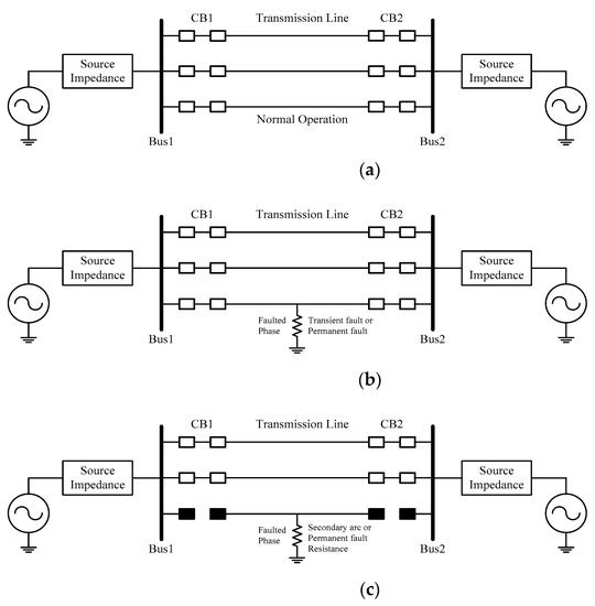
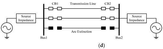
Figure 1.
Advanced adaptive single-pole auto-reclosing (ASPAR) operation sequence: (a) transmission line under normal operation; (b) single-pole to ground fault (transient or permanent); (c) isolation of the faulted phase through a conventional scheme; (d) extinction of the secondary arc due to a transient fault after an unknown time.
2.2. Secondary Arc
A primary arc caused by a transient single-pole to ground fault can be eliminated by the SPAR operation, which isolates the faulted phase from the power system. During the opening of the faulted phase, the voltage of the faulted-phase conductor is induced by capacitive and inductive mutual coupling between the faulted-phase conductor and sound-phase conductors. Because the air around a fault point is already ionized by the primary arc, this induced voltage creates and sustains a secondary arc for an unpredictable amount of time after the opening of the faulted phase. Numerous previous experimental studies and field tests have demonstrated that secondary arcs are an extremely complex electrical phenomenon that are influenced by various parameters [21]. In terms of protecting the power system, the secondary arc extinction time is considered the most important point in SPAR studies. The extinction time of a secondary arc depends on several factors, such as the magnitudes of the primary and secondary arc currents, recovery voltage, system voltage, interphase coupling, line compensation level, and length of the transmission line [21,22]. These factors can be affected by weather conditions, such as temperature, humidity, wind speed, and atmospheric conditions. Usually, the secondary arc is self-extinguished, but if the faulted phase is reclosed before the secondary arc is removed, the fault will reestablish, resulting in an unsuccessful reclosing. A prolonged delay (>2 s) in reclosing to compensate for the secondary arc extinction time can adversely affect the stability of the power system. When a secondary arc occurs due to a transient fault in the transmission line, in general, the secondary arc voltage has an irregular characteristic owing to the shoulder behavior of an arc current, with repeated intermittent arc extinction and re-ignition. Consequently, the secondary arc voltage exhibits a distorted shape, as demonstrated in Figure 2. This arc voltage waveform tends to differ from a typical voltage waveform that takes the shape of a sine wave under normal conditions. From the distorted shape of the voltage waveform, it can be concluded that the arc voltage contains harmonic components. In this study, these harmonic components are defined as a signature of the secondary arc voltage and are used as a factor to discern the fault type and detect the secondary arc extinction time.
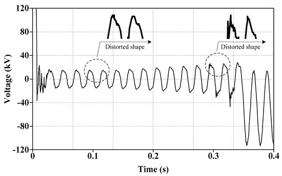
Figure 2.
Typical waveform of the secondary arc voltage.
2.3. Short-Time Fourier Transform
The fast Fourier transform (FFT), a signal processing tool, is the most commonly used mathematical technique for transforming a signal from the time domain to the frequency domain. The FFT method can calculate harmonic distortion and separate odd/even/inter-harmonics. FFT has been widely implemented in various power quality fields to analyze harmonic characteristics owing to its computational efficiency. However, the major disadvantage of using FFT arises when time data are needed in the frequency domain. In the time domain, frequency information cannot be obtained by FFT and vice versa, i.e., in the frequency domain, time data are not available [23].
One solution to this issue is STFT. STFT is commonly known as a sliding-window version of FFT. This method consists of sliding a window function over the signal and taking its Fourier transform (FT) for every half-window length. Accordingly, time information is available in the frequency domain with a resolution that depends on the width of the window function [23]. The window function, ω(t), with a size equal to each section is chosen, and it is placed at the beginning of the signal. The window shifts along the signal according to the hop size, repeating the FT for the new window with updated wave data. Moreover, based on the hop size and sampling, a number of samples will be released from the end of the windows. Then, the same number will be added to the front by making a time-based move. The following two equations describe the continuous and discrete forms of STFT, respectively [24]:
where x(n) is the input function, ω(n) is the window function, N is the number of FFT points, n is the number of input samples, and H is the hop size. STFT can also express the FT of the signal multiplied by the window function in a complex conjugate form. The time resolution depends on the hop size, as shown in Equation (3):
where k is the amount of data in the time axis, Nx is the data length, Noverlap is the window size minus the hop size, and Nω is the window length. The higher the value of k, the better the time resolution will be. In several studies, STFT has shown better results in terms of frequency selectivity compared with wavelets having fixed center frequencies and bandwidths [24,25]. Because STFT has a fixed frequency resolution for all frequencies, it has proven to be more suitable for harmonic analysis of voltage disturbances than other signal processing methods. As described above, STFT has several advantages and is superior for extracting the fundamental and harmonic components. Thus, STFT is effective for analyzing the harmonic characteristics related to power quality disturbances.
3. Fault Characteristics Based on Harmonic Analysis
3.1. Study System Conditions
The Korean 345 kV power transmission line illustrated in Figure 3 is considered a study system to simulate and analyze the harmonic characteristics of line faults. This transmission system has a single-machine infinite bus consisting of a 6300 MVA synchronized generator, step-up transformers, CBs, and 100 km of transmission line. Detailed parameters of the transmission line are listed in Table 1, and the study system is modeled using the EMTP software. In the study system, transient and permanent single-pole to ground faults are simulated. In the case of transient faults, the arc model proposed by Saul Goldberg is utilized [26]. The transient analysis of control systems (TACS) source and MODELS library in the EMTP software are used to implement the realistic nonlinear primary arc and secondary arc [20,21]. In addition, a linear fault resistance is applied to represent a permanent fault event. The total length of the transmission line is 100 km, and the fault location is 10% the length of the transmission line, i.e., at 10 km. For all the fault cases, a single-pole to ground fault occurs at t = 0.2 s. The fault is cleared after four cycles from the fault inception time, and only single-pole operation of the CBs is considered.
Figure 3.
Actual Korean 345 kV transmission study system.

Table 1.
The 345 kV transmission line parameters.
3.2. Harmonic Analysis of the Faulted-Phase Voltage (Transient/Permanent)
First, the voltage waveforms of the faulted phase for transient and permanent faults are analyzed. For this analysis, two fault simulations are performed for the 345 kV study system described in Figure 3 and Section 3.1, and the simulation results are presented in Figure 4. Figure 4 shows the result for one of the many simulation cases. In terms of basic fault phenomena, we confirmed that an arc voltage caused by a secondary arc still exists after tripping the CB in the transient fault situation. Then, a recovery voltage is observed after final extinction of the secondary arc. However, for the permanent fault, the fault persists, and thus the system voltage does not recover to a steady state even after the voltage drops sharply following tripping of the CB. Depending on the simulation conditions, the magnitude of the voltage or the shape of the waveform can be varied. However, a series of processes in which the secondary arc occurs after CBs trip following a fault, and then the recovery voltage arises after the secondary arc is eliminated are a general trend for fault covered in this study.
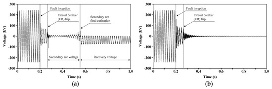
Figure 4.
Voltage waveform of the faulted phase: (a) transient fault; (b) permanent fault.
Second, a harmonic analysis of the faulted-phase voltage is performed for both the transient and permanent faults. To identify several significant features, THD analysis is performed. The distortion rate of the signal, i.e., the normalized value of the harmonic ratio contained in a signal, is called the THD. THD can be defined as the relative signal energy present at non-fundamental frequencies, and this factor is commonly utilized to quantify waveform distortion in the power quality analysis field. In general, the THD of a voltage is expressed by the following equation:
where V means the RMS value of the voltage. V1 and VH represent the RMS of the fundamental wave and the RMS of the harmonics included in the signal, respectively. For general power system analyses, up to fiftieth harmonics can be considered. However, the signal energy is drastically reduced at high harmonic frequencies, and thus most of the THD energy is usually contained in low-order harmonic frequencies [27,28]. In addition, dealing with a wide range of frequencies makes the computational process more complex and burdensome. For these practical reasons, it is reasonable to only consider the low-order harmonics, which are sufficient to verify the major features of the harmonics of the faulted-phase voltage. In this study, the THD factor is calculated using harmonics up to the seventh order. To extract the harmonic components and calculate the THD from a fault voltage waveform, STFT is applied. The sampling frequency is 7.2 kHz, and the size of the window function is set to 16.67 ms, which is approximately one cycle at 60 Hz. Figure 5 depicts the results of the THD calculation for the voltage waveforms in Figure 4.
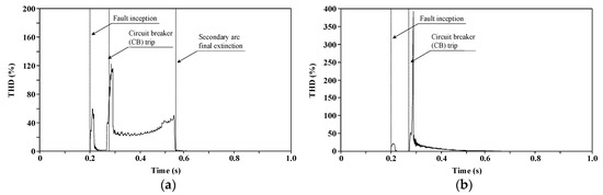
Figure 5.
Total harmonic distortion (THD) calculation results for the waveforms shown in Figure 4: (a) transient fault; (b) permanent fault.
In Figure 5, three simple features are observed:
- The THD of the faulted-phase voltage during the transient fault exhibits a sharp increase and decrease at the time when the CB is tripped, after which it gradually increases until the final extinction of the secondary arc.
- The THD of the faulted phase voltage during the transient fault depicts a drastic decrease immediately after the final extinction of the secondary arc.
- In the case of the permanent fault, the THD of the faulted-phase voltage shows a rapid increase only at the time when the CB is tripped and then continues to decrease.
A common characteristic verified by the above THD analysis is that the increase and decrease of the THD are repeated locally in both faults. In addition, there are some different trends between the two faults: (1) the magnitudes of the increase and decrease of the THD differ, and (2) there is variation in the frequency of the THD. These definite signatures can be utilized as important factors for distinguishing whether the fault type is transient or permanent. In the next section, Sequence 1 algorithm for discrimination of the fault type is introduced by applying the aforementioned features.
Furthermore, the characteristics of the harmonic components contained in the secondary arc voltage caused by the transient fault are analyzed. To identify certain clear features that can be utilized to detect the extinction time of the secondary arc, components up to the seventh harmonic are extracted for the transient fault case, and the results are shown in Figure 6. The major characteristics derived from the extracted odd/even-order harmonics can be summarized as follows:
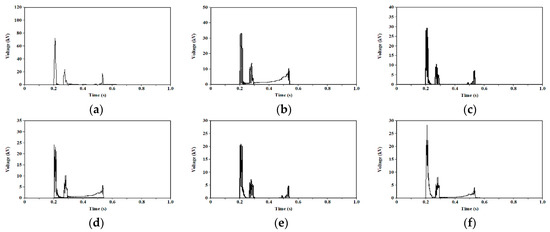
Figure 6.
Harmonics calculation results for the waveform in Figure 4a: (a) 2nd harmonic; (b) 3rd harmonic; (c) 4th harmonic; (d) 5th harmonic; (e) 6th harmonic; (f) 7th harmonic.
- In the case of even-order harmonics of the faulted phase, the harmonics is quite large near the extinction point of the secondary arc, while the magnitude is considerably small before that.
- The odd-order harmonics of the faulted phase are not only relatively large around the extinction point of the secondary arc, but also have a certain value before that.
- After secondary arc extinction, there is a significant difference in the harmonic variation between the odd- and even-order harmonics.
- A common characteristic is that the higher the order of the harmonics, the lower the number of harmonics included in the voltage waveform will be. In other words, most of the harmonic components tend to be distributed toward the low-order harmonics.
- Therefore, when analyzing and utilizing the harmonic components contained in the secondary arc voltage during the transient fault condition, it is sufficient to consider the low-order harmonics.
By analyzing the difference in the THD variation according to the fault type and the characteristics of the harmonics in the secondary arc voltage, we can verify the important features in each fault situation. During the transient fault, the voltage of the faulted phase fluctuates more frequently because of the intermittent extinction and re-ignition of the secondary arc, including the occurrence of a recovery voltage. Consequently, the change in the THD is more severe than that for the permanent fault. In addition, in the case of a transient fault, the magnitudes of the odd- and even-order harmonics are significantly different before and after the extinction of the secondary arc. In particular, the difference in the harmonics is significantly polarized after the secondary arc extinction. In Section 4, several new factors are defined to normalize these features. Based on these results, an auto-reclosing scheme is proposed for both discrimination of the fault type and detection of the secondary arc extinction time.
4. New Adaptive Auto-Reclosing Scheme
The ASPAR scheme proposed in this study consists of two sequences as shown in Figure 7. The first sequence determines whether a fault type is transient or permanent. In this step, the fault type is accurately discriminated. In the event of a permanent fault, a reclosing operation is not performed to protect the system stability from being affected by an unnecessary reclosing. In the case of a transient fault, however, the final extinction time of the secondary arc is detected through the second sequence. This step is aimed at determining the instant of the optimal reclosing operation. Two algorithms are applied to perform the above operations for the two sequences. The basic concept of the total operation of the developed algorithms is based on the THD and harmonic features of the faulted-phase voltage according to the fault conditions analyzed in the previous section. Details of the suggested algorithms are described in the sections below.
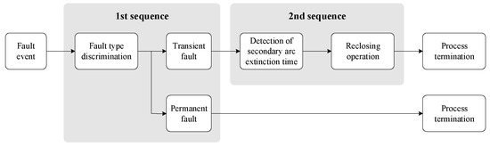
Figure 7.
Total operation concept of the proposed ASPAR scheme.
4.1. Algorithm for Discrimination of the Fault Type—Sequence 1
The primary function of the Sequence 1 algorithm is to accurately distinguish the fault type and then rapidly prepare the subsequent operation for a transient fault. In addition, it prevents unnecessary reclosing caused by a malfunction of the protective relay for a permanent fault. This algorithm utilizes the pattern in which the THD of the faulted-phase voltage locally increases and decreases during a fault period. To represent these THD variations, a new variable called ΔTHD is defined as follows:
where THDavg is the average value of the THD during one cycle, THDavg(i) is the value of THDavg for the current cycle, and THDavg(i–1) is the value of THDavg calculated in the previous cycle. The reason for deriving THDavg is that, as mentioned previously, the THD of the faulted-phase voltages in both transient and permanent faults repeatedly increase and decrease. As a result, an overall pattern of changes in the THD can be identified by analyzing the variation and deviation based on the average value of the THD. Next, new count functions, Count_P and Count_M, are defined as indicators to quantify the frequency of the changes in the THD during the fault period. If ΔTHD has a positive value, Count_P is increased by 1 for every sample, whereas Count_M is increased by 1 for every sample when ΔTHD has a negative value. In general, the magnitude or shape of a harmonic varies considerably according to the voltage fluctuation and fault duration that depend on the fault type, which can result in THD variations. If limited to the fault type, the THD variation is rather noticeable, particularly in the fault duration section. Thus, in this study, these features are simply generalized using Count_P and Count_M. Moreover, these two factors are used as the major elements to distinguish a significant characteristic between the transient and permanent faults.
Figure 8 depicts the Count_P of the THD for the voltage waveforms of the transient and permanent faults in Figure 4. Count_P in the transient fault continues to increase after the CB is tripped until the secondary arc is completely extinguished. On the other hand, Count_P in the permanent fault has a maximum value of 1 after the CB is tripped, and it maintains a value of approximately zero for most of the duration. Therefore, the cases in which Count_P is greater and Count_P continues to increase over a certain time can be discriminated as transient faults. In other words, Count_P, which has a relatively high variation in the transient fault situation, can be utilized as a criterion for detecting transient faults. Accordingly, we present a threshold value, λP, which is a time limit to decide whether the fault type is transient or not. If Count_P is greater than λP, the case is considered a transient fault. To set the value of λP, we refer to the deionizing time defined in IEEE Std C37.104-2002 [29], using which we derive λP, as in Equation (6):
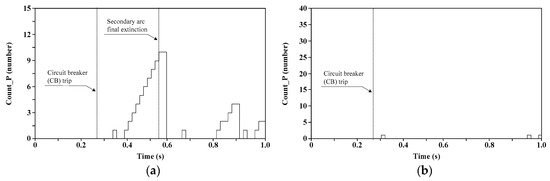
Figure 8.
Results of Count_P for transient and permanent faults: (a) transient; (b) permanent.
In Equation (6), VL-L and WP represent the nominal voltage of the power system and weight factor applied to the deionizing time for identification of transient faults, respectively. To select an appropriate WP, various simulations are performed, and it is confirmed that the maximum value of Count_P within the secondary arc period is generally between 35.6% and 60.1% of the total secondary arc duration. This means that WP should be set at a value of 0.601 or less because the time for final extinction of the secondary arc must also be considered to perform an opportune reclosing operation, although a transient fault can be recognized effectively at approximately 60.1% of the secondary arc duration. Based on diverse simulation cases for determining the value of WP, it is set to between 0.45 and 0.55 because this range has the highest rates of fault detection and reclosing success.
Figure 9 depicts the Count_M of the THD for the voltage waveforms of the transient and permanent faults in Figure 4. As shown in this figure, Count_M in the transient fault exhibits a short increase immediately after the CB is tripped and then does not have any value for the secondary arc period. Meanwhile, Count_M in the permanent fault increases continuously after the CB is tripped. Therefore, the event in which Count_M is greater and lasts over a certain time can be determined as a permanent fault, and the Count_M index, which shows a relatively high variation in permanent events, can be used as a criterion for detecting permanent faults.
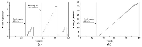
Figure 9.
Results of Count_M for transient and permanent faults: (a) transient; (b) permanent.
Similar to the case of the transient fault, we define a threshold value, λM, for detecting a permanent fault based on the deionizing time in Equation (7), where WM is the weight factor applied to the deionizing time for identification of a permanent fault. In simulations to select an appropriate WM value, the maximum value of Count_M within the secondary arc period is generally between 28.2% and 44.4% of the total secondary arc duration. Therefore, WM must be set at a value of 0.44 or greater. Based on diverse simulation cases for determining the value of the WP index, WM is set to between 0.55 and 0.65:
Figure 10 illustrates a diagram of the proposed scheme for discriminating between transient and permanent faults using the THD features of the faulted-phase voltage. The proposed scheme only acquires voltage information from the transmission line. If a single-pole to ground fault is detected, the CB of the faulted phase is tripped. Using the faulted-phase voltage, the THDavg during the fault duration is calculated for every sample and then compared with the sample in the previous cycle to derive the ΔTHD, which indicates the variation in the THD. Whenever ΔTHD has a positive value, Count_P is increased by 1 for every sample. If Count_P exceeds a time threshold, λP, the fault type is classified as transient, and the Sequence 2 process is performed to detect the secondary arc extinction time for performing the reclosing. If ΔTHD has a negative value, however, Count_M is increased by 1 for every sample. If Count_M persists until a time threshold, λM, the fault type is classified as permanent. In the case of a permanent fault, reclosing is not performed because unnecessary reclosing operations can reduce the power system stability.
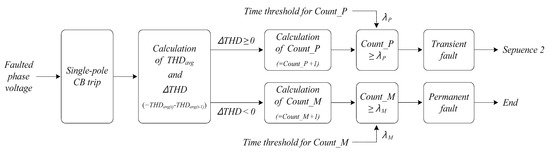
Figure 10.
Diagram of the proposed scheme for discrimination of the fault type.
4.2. Algorithm for Detection of the Secondary Arc Extinction—Sequence 2
The purpose of the Sequence 2 algorithm is to detect the final extinction time of the secondary arc arising from a transient fault. This algorithm utilizes the voltage variation patterns for each harmonic order of the secondary arc voltage wave analyzed in Section 3.2. To utilize the aforementioned features, new factors, OOHD and EOHD, are defined, which indicate the sum of the odd-order harmonic distortion and the sum of the even-order harmonic distortion, respectively. In power transmission lines in a stable condition, in general, the THD tends to have a low value, and a nearly equal proportion of odd- and even-order components are present in the harmonics. In the transient fault condition, however, the THD of the faulted-phase has a high value, and the secondary arc voltage waveform exhibits a significantly distorted shape. This is because components of the even-order harmonics are over-represented compared to those of the odd-order harmonics. These features can be identified through the analysis in Section 3.2. For the development of the Sequence 2 algorithm, OOHD and EOHD are used to compare the difference between the odd- and even-order harmonics by expressing them as normalized indicators. OOHD and EOHD can be expressed as follows:
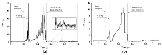
The calculation results for the OOHD and EOHD of the voltage waveform in Figure 4a are presented in Figure 11. As shown in Figure 11, OOHD maintains a certain value after the CB is tripped. It increases slightly near the secondary arc extinction point and then decreases rapidly. Meanwhile, EOHD remains at a low value after the CB is tripped; it shows a rapid increase near the secondary arc extinction point and then decreases again. By comparing OOHD and EOHD patterns in the fault situation, two features are identified. First, the two factors exhibit different characteristics during the secondary arc period, and a large deviation exists between them. Second, the deviation gradually decreases after extinction of the secondary arc. Thereafter, OOHD and EOHD have approximately equal values starting from when the recovery voltage arises. Using these features, particularly the second feature, the point where the OOHD and EOHD ratios in the secondary arc voltage become nearly identical can be defined as the extinction time of the secondary arc. Accordingly, a new variable defined as a harmonic ratio (HR_THD) is utilized, as shown in Equation (10):
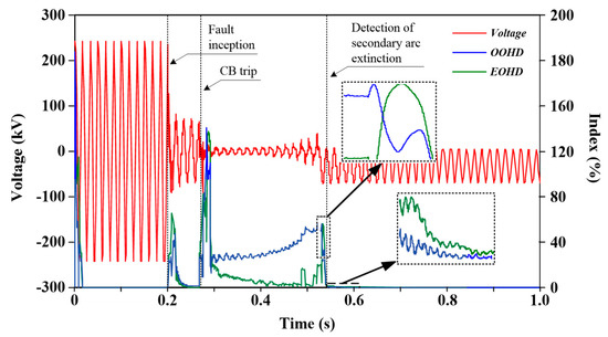
Figure 11.
OOHD and EOHD results for the voltage waveform in Figure 4a.
Figure 12a demonstrates the results for the HR_THD derived from Figure 4a. To express the waveform of HR_THD more clearly, HR_THD(f), which applies a filter to HR_THD, is presented in Figure 12b. The value of HR_THD(f) is considerably low only during the normal condition period prior to the fault inception and after the arc extinction, at which points the value of HR_THD(f) is less than 1. In conclusion, based on HR_THD(f), it is possible to determine whether the secondary arc has been extinguished by detecting a section in which the value of HR_THD(f) enters a stable range.
The procedure to detect the final extinction time of the secondary arc in the faulted phase is demonstrated in Figure 13. First, the THD data acquired in the Sequence 1 algorithm are separated into OOHD and EOHD. In general, the proportions of odd- and even-order harmonics present in the voltage are similar in the steady state. In the event of disturbances, such as faults, however, the harmonic components in the fault voltage increase sharply, causing a severe imbalance between the odd- and even-order harmonics present in the fault voltage. In the case of a transient fault, the ratio of the two harmonic components during the secondary arc period is also unbalanced. Once the secondary arc is extinguished and the system voltage stabilizes, the proportions of odd- and even-order harmonics become similar again, and this point can be determined as the time of the secondary arc extinction. To utilize these features, HR_THD is calculated by comparing the proportions of odd- and even-order harmonic components. To determine the instant of the secondary arc extinction accurately, an additional filtering process is conducted to remove the uncertain noise components and outliers. The HR_THD(f) derived by these processes determines the secondary arc extinction time based on the threshold value, λf, and the reclosing can then be conducted through a trip signal.
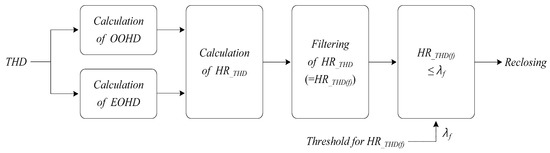
Figure 13.
Diagram of the proposed scheme for detection of secondary arc extinction.
5. Simulations and Results
5.1. Simulations in a 345 kV Power Transmission System
To verify the proposed ASPAR scheme, the 345 kV study system illustrated in Figure 3 is used for simulations. To evaluate the performance of the algorithms for the length of the transmission line and fault location, various simulation cases are considered. The total length of the transmission line is classified into cases of 100 and 200 km, and each fault location case is simulated at varying distances from a transmission point. For all cases, the detailed simulation conditions are presented in Table 2.
Table 2.
Simulation conditions.
Figure 14a shows the simulation results for the faulted-phase voltage measured at a relay point on a transmitting terminal of the transmission line when a transient fault occurs 10 km from the transmission point. In addition, Figure 14b presents the calculated values of THD and HR_THD(f).
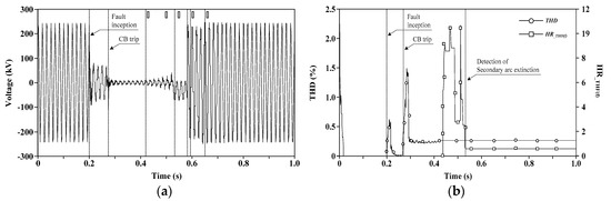
Figure 14.
Simulation results for a transient fault: (a) faulted-phase voltage; (b) THD and HR_THD(f).
In Figure 14a, a fault occurs at t = 0.2 s, and then a CB on the transmission line is tripped after approximately four cycles. In Figure 14b, the THD is calculated for the voltage waveform of the faulted phase to identify the fault type using the Sequence 1 algorithm. When a fault occurs, the proposed scheme detects the fault through a change in voltage and utilizes the characteristics that the THD of the voltage waveform shows repeated increases and decreases. Even if the magnitude of the voltage THD in Figure 14b is within the normal range, from a range of background harmonic distortion perspective [30], it is possible to detect the fault type by catching the repeated and continuous variation of THD caused by the fault even in normal situations. In Sequence 1 algorithm, if the fault is identified as a transient type through the classification process for transient and permanent faults, a calculation of HR_THD(f) using the Sequence 2 algorithm is begun to detect the extinction time of the secondary arc and prepare the subsequent reclosing operation. When the final extinction time of the secondary arc is derived from the HR_THD(f) calculation results, the reclosing of the CB is conducted through an operation command for a reclosing relay. A series of processes in which the operation sequence from fault detection to termination of the reclosing is successfully obtained using the proposed reclosing scheme are presented in Figure 14a. In other words, the proposed method is operated over the following five steps, after which the system voltage of the power transmission line is successfully recovered to a steady state.
- Discrimination of a transient fault (Sequence 1 algorithm);
- Detection of the final extinction of the secondary arc (Sequence 2 algorithm);
- Reclosing of the leader-end CB;
- Voltage check;
- Reclosing of the follower-end CB.
Further simulation results are presented in Table 3 and Table 4, which indicate that the proposed ASPAR algorithm accurately distinguishes the fault type in all of the simulation cases. For transient faults, reclosing is normally performed after detection of the secondary arc extinction time. In Korea, the traditional auto-reclosing method, which uses a constant predetermined time called a “fixed dead time” for the arc extinction, has been applied in the transmission system. The criterion for the conventional SPAR in the 345 kV power transmission system is based on a fixed dead time of 48 cycles, i.e., 0.8 s. With the implementation of the proposed ASPAR scheme, the simulation results for the transient faults indicate that a series of operations from the detection of the fault type and secondary arc extinction time to the reclosing operation can be completely terminated within the fixed dead time of the current SPAR method. Because the fault type and final extinction of the secondary arc can be identified within about 0.5 s after fault occurrence in all the simulation cases, there is a sufficient time margin to perform the reclosing operation before the fixed dead time, although the CBs are reclosed immediately within a few cycles after detection of the secondary arc extinction. However, the proposed ASPAR process is not performed if the fault discrimination step identifies a permanent fault. Through these simulation results, we can verify that the proposed ASPAR scheme identifies the fault type and determines whether reclosing should be performed based on the fault type accurately. This means that application of the proposed ASPAR method can reduce unnecessary dead time and restore a power system to the steady state more quickly than the traditional auto-reclosing based on a fixed dead time. In addition, it can contribute to enabling efficient system operation and increased system stability.
Table 3.
Simulation results for verification of the ASPAR scheme in a 345 kV transmission line (100 km).
Table 4.
Simulation results for verification of the ASPAR scheme in a 345 kV transmission line (200 km).
5.2. Simulations in a 765 kV Power Transmission System
To expand the verification of the proposed reclosing scheme, additional simulations are performed for an actual 765 kV transmission system in Korea illustrated in Figure 15. Two parallel 765 kV transmission lines are located between the Sin-Gapyung and Sin-Taebaek substations with a total line length of 160 km. Each fault case is simulated by moving the fault location at intervals of 10 km from a transmission point. The other simulation conditions are the same as those in Table 2.
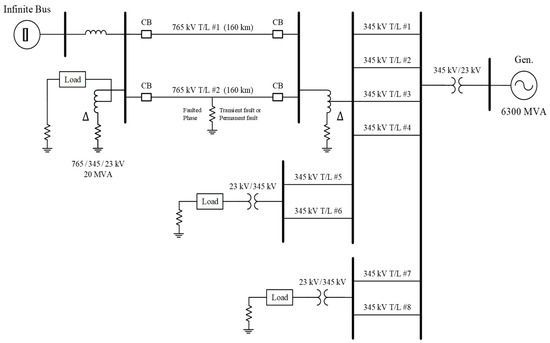
Figure 15.
Actual 765 kV transmission system in Korea.
Table 5 summarizes the simulation results for the 765 kV transmission system. Similar to the simulations with the 345 kV system, the proposed scheme can distinguish the fault type accurately for all the considered cases. For transient faults, reclosing operations are performed successfully, as indicated in Table 5. Currently, the criterion for conventional SPAR in the Korean 765 kV transmission system applies a fixed dead time of 60 cycles, i.e., 1.0 s. From the above results, in the case of a transient fault, the proposed ASPAR scheme can conduct the reclosing faster than the current dead time of 1.0 s even though the CBs are reclosed within a few cycles after identification of the secondary arc extinction. These results demonstrate that the ASPAR scheme proposed in this study can ensure superior performance even at various transmission system voltage levels, and the proposed scheme demonstrates significant effectiveness for protecting power systems from both transient and permanent single-pole to ground faults.
Table 5.
Simulation results for verification of the ASPAR scheme in a 765 kV transmission line (160 km).
6. Conclusions
In this study, an advanced ASPAR scheme is proposed to protect transmission power systems from single-pole to ground faults. With application of the STFT signal processing tool, the proposed scheme utilizes the THD factor and odd/even-order harmonic components of the faulted-phase voltage to discern the fault type and detect the secondary arc extinction, respectively. Based on these factors, an ASPAR scheme comprising two coordinated algorithms is proposed, and various fault simulations are conducted to verify its performance. From the simulation results for actual 345 and 765 kV Korean transmission study systems, we verify that the proposed scheme can accurately identify the fault type and accurately determine whether reclosing must be performed based on the fault type. In addition, implementation of the developed ASPAR method can reduce unnecessary dead time and restore the power system to the steady state more rapidly than the conventional auto-reclosing method based on a fixed dead time. Therefore, implementing the proposed ASPAR scheme in power transmission line protection relays can contribute to enhancing the power system stability and enabling efficient system operation.
Author Contributions
Conceptualization, methodology, C.-H.K. and J.H.; software, validation, J.H and C.-M.L.; formal analysis, J.H. and C.-H.K.; data curation, J.H.; Writing—Original draft preparation, J.H.; Writing—Review and editing, J.H.; supervision, C.-H.K. All authors have read and agreed to the published version of the manuscript.
Funding
This work was supported by the National Research Foundation of Korea (NRF) grant funded by the Korea government (MSIP) (No. 2018R1A2A1A05078680). This work has also supported by “Human Resources Program in Energy Technology” of the Korea Institute of Energy Technology Evaluation and Planning (KETEP), granted financial resource from the Ministry of Trade, Industry & Energy, Republic of Korea (No. 20184030202190).
Institutional Review Board Statement
Not applicable.
Informed Consent Statement
Not applicable.
Data Availability Statement
Not applicable.
Conflicts of Interest
The authors declare no conflict of interest.
References
- Ahn, S.-P.; Kim, C.-H.; Aggarwal, R.; Johns, A. An alternative approach to adaptive single pole auto-reclosing in high voltage transmission systems based on variable dead time control. IEEE Trans. Power Deliv. 2001, 16, 676–686. [Google Scholar] [CrossRef]
- Jamali, S.; Baayeh, A.G. Detection of secondary arc extinction for adaptive single phase auto-reclosing based on local voltage behaviour. IET Gener. Transm. Distrib. 2017, 11, 952–958. [Google Scholar] [CrossRef]
- Jamali, S.; Parham, A. New approach to adaptive single pole auto-reclosing of power transmission lines. IET Gener. Transm. Distrib. 2010, 4, 115. [Google Scholar] [CrossRef]
- Elmore, W.A. Protective Relaying Theory and Applications; ABB Power T&D Company Inc.: New York, NY, USA, 1994. [Google Scholar]
- Milne, K. Single-Pole Reclosing Tests on Long 275-Kv Transmission Lines. IEEE Trans. Power Appar. Syst. 1963, 82, 658–661. [Google Scholar] [CrossRef]
- Peterson, H.A.; Dravid, N.V. A Method for Reducing Dead Time for Single-Phase Reclosing in EHV Transmission. IEEE Trans. Power Appar. Syst. 1969, 286–292. [Google Scholar] [CrossRef]
- Kappenman, J.G.; Sweezy, G.A.; Koschik, V.; Mustaphi, K.K. Staged fault tests with single phase reclosing on the Winnipeg-Twin cities 500 kV interconnection. IEEE Trans. Power Appar. Syst. 1982, PAS-101, 662–673. [Google Scholar] [CrossRef]
- Esztergalyos, J.; Andrichak, J.; Colwell, D.H.; Dawson, D.C.; Jodice, J.A.; Murray, T.J.; Mustaphi, K.K.; Nai1, G.R.; Politis, A.; Pope, J.W.; et al. Single-phase tripping and auto reclosing of transmission-lines IEEE committee report. IEEE Trans. Power Deliv. 1992, 7, 182–192. [Google Scholar]
- Jamali, S.; Ghaffarzadeh, N. Adaptive single pole auto-reclosing using discrete wavelet transform. Eur. Trans. Electr. Power 2010, 21, 973–986. [Google Scholar] [CrossRef]
- Radojevic, Z.M.; Shin, J.R. New digital algorithm for adaptive re-closing based on the calculation of the faulted phase voltage total harmonic distortion factor. IEEE Trans. Power Deliv. 2007, 22, 37–41. [Google Scholar] [CrossRef]
- Zhalefar, F.; Zadeh, M.R.D.; Sidhu, T.S. A High-Speed Adaptive Single-Phase Reclosing Technique Based on Local Voltage Phasors. IEEE Trans. Power Deliv. 2015, 32, 1203–1211. [Google Scholar] [CrossRef]
- Khodadadi, M.; Noori, M.R.; Shahrtash, S.M. A Noncommunication Adaptive Single-Pole Autoreclosure Scheme Based on the ACUSUM Algorithm. IEEE Trans. Power Deliv. 2013, 28, 2526–2533. [Google Scholar] [CrossRef]
- Lin, X.; Liu, H.; Weng, H.; Liu, P.; Wang, B.; Bo, Z.Q. A Dual-Window Transient Energy Ratio-Based Adaptive Single-Phase Reclosure Criterion for EHV Transmission Line. IEEE Trans. Power Deliv. 2007, 22, 2080–2086. [Google Scholar] [CrossRef]
- Zadeh, M.R.D.; Rubeena, R. Communication-Aided High-Speed Adaptive Single-Phase Reclosing. IEEE Trans. Power Deliv. 2012, 28, 499–506. [Google Scholar] [CrossRef]
- Elkalashy, N.I.; Darwish, H.A.; Taalab, A.M.I.; Izzularab, M.A. An adaptive single pole auto-reclosure based on zero sequence power. Electr. Power Syst. Res. 2007, 77, 438–446. [Google Scholar] [CrossRef]
- Yu, I.K.; Song, Y.H. Wavelet analysis and neural network based adaptive single pole auto reclosure scheme for EHV transmission systems. Int. J. Electr. Power Energy Syst. 1998, 20, 465–474. [Google Scholar] [CrossRef]
- Lin, X.; Liu, P. Method of distinguishing between instant and permanent faults of transmission lines based on fuzzy decision. In Proceedings of the Proceedings of EMPD’ 98. 1998 International Conference on Energy Management and Power Delivery (Cat. No.98EX137), Singapore, 5 March 1998. [Google Scholar]
- Aggarwal, R.; Johns, A.; Song, Y.; Dunn, R.; Fitton, S. Neural-network based adaptive single-pole autoreclosure technique for EHV transmission systems. IEE Proc. Gener. Transm. Distrib. 1994, 141, 155–160. [Google Scholar] [CrossRef]
- Yu, I.K.; Song, Y.H. Wavelet transform and neural network approach to developing adaptive single-pole auto-reclosing schemes for EHV transmission systems. IEEE Power Eng. Rev. 1998, 18, 62–64. [Google Scholar] [CrossRef]
- Lin, X.; Weng, H.; Liu, H.; Lu, W.; Liu, P.; Bo, Z. A Novel Adaptive Single-Phase Reclosure Scheme Using Dual-Window Transient Energy Ratio and Mathematical Morphology. IEEE Trans. Power Deliv. 2006, 21, 1871–1877. [Google Scholar] [CrossRef]
- Nikoofekr, I.; Sadeh, J. Determining secondary arc extinction time for single-pole auto-reclosing based on harmonic signatures. Electr. Power Syst. Res. 2018, 163, 211–225. [Google Scholar] [CrossRef]
- Montanari, A.A.; Tavares, M.C.; Portela, C.M. Secondary arc voltage and current harmonic content for field tests results. Int. Conf. Power Syst. Transients 2009. Available online: https://www.ipstconf.org/Proc_IPST2009.php (accessed on 27 February 2021).
- Kostov, M.; Gegov, B.; Atanasovski, M.; Petkovski, M. Short Time Fourier Transform for Power Disturbances Analysis. In Proceedings of the International Scientific Conference on Information, Communication and Energy Systems and Technologies, Sofia, Bulgaria, 24–26 June 2015. [Google Scholar]
- Ashouri, M.; Silva, F.F.D.; Bak, C.L. Application of short-time Fourier transform for harmonic-based protection of meshed VSC-MTDC grids. J. Eng. 2019, 2019, 1439–1443. [Google Scholar] [CrossRef]
- Ingale, R. Harmonic Analysis Using FFT and STFT. Int. J. Signal Process. Image Process. Pattern Recognit. 2014, 7, 345–362. [Google Scholar] [CrossRef]
- Goldberg, S.; Horton, W.; Tziouvaras, D. A computer model of the secondary arc in single phase operation of transmission lines. IEEE Trans. Power Deliv. 1989, 4, 286–295. [Google Scholar] [CrossRef]
- Babaei, E.; Hosseini, S.H.; Gharehpetian, G.B. Reduction of THD and low order harmonics with symmetrical output current for single-phase ac/ac matrix converters. Int. J. Electr. Power Energy Syst. 2010, 32, 225–235. [Google Scholar] [CrossRef]
- Jeevananthan, S.; Nandhakumar, R.; Dananjayan, P. Inverted sine carrier for fundamental fortification in PWM inverters and FPGA based implementations. Serbian J. Electr. Eng. 2007, 4, 171–187. [Google Scholar] [CrossRef]
- IEEE Guide for Automatic Reclosing of Line Circuit Breakers for AC Distribution and Transmission Lines; IEEE Std C37.104-2002; IEEE: New York, NY, USA, 2002; Available online: https://ieeexplore.ieee.org/document/1193340 (accessed on 27 February 2021).
- IEEE Recommended Practice and Requirements for Harmonic Control in Electric Power Systems; IEEE Std 519-2014; IEEE: New York, NY, USA, 2014; Available online: https://ieeexplore.ieee.org/document/6826459 (accessed on 27 February 2021).
Publisher’s Note: MDPI stays neutral with regard to jurisdictional claims in published maps and institutional affiliations. |
© 2021 by the authors. Licensee MDPI, Basel, Switzerland. This article is an open access article distributed under the terms and conditions of the Creative Commons Attribution (CC BY) license (http://creativecommons.org/licenses/by/4.0/).