Adaptive Fuzzy Approximation Control of PV Grid-Connected Inverters

Abstract

Three-phase inverters are widely used in grid-connected renewable energy systems. This paper presents a new control methodology for grid-connected inverters using an adaptive fuzzy control (AFC) technique. The implementation of the proposed controller does not need prior knowledge of the system mathematical model. The capabilities of the fuzzy system in approximating the nonlinear functions of the grid-connected inverter system are exploited to design the controller. The proposed controller is capable to achieve the control objectives in the presence of both parametric and modelling uncertainties. The control objectives are to regulate the grid power factor and the dc output voltage of the photovoltaic systems. The closed-loop system stability and the updating laws of the controller parameters are determined via Lyapunov analysis. The proposed controller is simulated under different system disturbances, parameters, and modelling uncertainties to validate the effectiveness of the designed controller. For evaluation, the proposed controller is compared with conventional proportional-integral (PI) controller and Takagi–Sugeno–Kang-type probabilistic fuzzy neural network controller (TSKPFNN). The results demonstrated that the proposed AFC showed better performance in terms of response and reduced fluctuations compared to conventional PI controllers and TSKPFNN controllers.

1. Introduction

Nowadays, renewable energy sources (RES) such as photovoltaic (PV) solar systems, wind turbines, and others are integrated into conventional power systems to avoid the high cost of constructing new or expanded facilities [1]. The final stage of the integration of PV systems consists of DC-AC inverters. Special consideration for inverter topologies and controls is required to preserve the network stability and to achieve acceptable dynamic performance of the voltage and frequency [2]. Different controllers for micro-grid inverters during grid-connected and islanded operation modes have been investigated in previous studies [3,4]. Corresponding to behavior and operating conditions of the electrical grid, the controllers of the inverter system can be classified as linear, non-linear, robust, adaptive, predictive, and intelligent controllers [5]. Various types of linear controllers for micro-grid inverters including classical controllers, Proportional Resonant (PR) controllers, and Linear Quadratic Gaussian (LQG) controllers were reported [6,7,8]. Non-linear controllers for grid-connected inverter systems (GCIS) such as sliding mode, feedback linearization, and hysteresis controllers have been proposed in [9,10,11,12,13]. In [14], a current-control is proposed for voltage-source inverters using the H_∞ robust control technique. Additionally, adaptive control techniques and model predictive controllers for grid-connected and standalone inverters were reported in [15,16,17,18]. In all studies referred to, the proposed non-linear controllers showed better performance when compared with linear controllers’ performance. The main drawback of nonlinear control methods is that they rely on the system mathematical model and system parameters availability.

Intelligent control systems including neural network controllers, repetitive controllers, fuzzy logic controllers (FLCs), and autonomous controllers are introduced for nonlinear systems control. The advantage of intelligent controllers is that they do not rely on the system mathematical model and they can handle many nonlinear and uncertain systems. In [19], a discrete-time repetitive controller (RC) was proposed to improve the output current and to overcome the drawback of using a linear PI controller in the presence of non-linearities in the system components. Type-1 and Type-2 FLCs have been widely used in various applications and have achieved remarkable success in managing higher levels of uncertainty [20,21,22,23,24,25]. FLC applications also include intelligent control for marine applications, traction diesel engines, robotic control, internet bandwidth control, industrial system controllers, power management and electrical control, aircraft control evolutionary computing, and DC-DC converters. Moreover, type-2 fuzzy logic has also proven successful in clinical diagnosis, differential diagnosis, and nursing evaluation in the health field [26].

For GCIS, different FLCs were presented in [27,28,29]. In [28], the real time testing for FLC for three phase grid-connected inverters to control the voltage and the current was presented. The results demonstrated FLC ability to generate high-quality PV power while maintaining the power factor of unity. A grid side inverter system control using a simple FLC that works well for grid interconnected variable speed wind generators was proposed in [29]. In another work, type-2 FLC (T2FLC) was implemented to control a DC-DC buck converter [30]. For PV systems, interval T2FLC (IT2FLC) based on maximum power point tracking (MPPT) method was proposed in [31]. In addition, the work in [32] implemented a T2FLC as a MPPT to handle the rules’ uncertainties during high weather condition variations. The proposed MPPT based on the FLC showed a faster response in the transient response and a stable steady state. A further IT2FLC was developed for single phase grid connected PV systems in [33], where IT2FLC was used as MPPT algorithm. Simulation results showed that the proposed IT2FLC-based MPPT controller has a fast transient response.

In [34], an FLC for inverters in PV applications was presented; the work discussed several factors and challenges and provided guidelines for developing capable and effective inverter control systems.

Moreover, a fuzzy neural network controller based on the Takagi–Sugeno–Kang type approach presented to control the active and reactive power of three-phase grid-connected PV systems during grid faults was reported in [35,36].

Furthermore, to overcome the disadvantages of conventional controllers for uncertain nonlinear systems, adaptive fuzzy control (AFC) techniques were proposed to control uncertain nonlinear systems [37,38]. Due to its advantage in handling complex uncertain nonlinear systems, researchers have used the AFC techniques in different applications [39,40,41,42,43]. The AFC technique was applied for induction motor control in [39], the optimal power conversion control for standalone wind energy conversion systems in [40], permanent magnet synchronous motor control, and fuzzy fault-tolerant switched systems in [41,42]. To the best of the authors’ knowledge, there is no reported work available that describe the application of AFC to the GCIS. This motivates the authors to propose an AFC scheme that exploits the concept of the multi-input multi-output (MIMO) feedback linearization and the approximation capability of fuzzy systems. PV GCIS are highly nonlinear and uncertain systems due to the intermittent nature of the PVand the inverter pulse width-modulation (PWM) technique. Without fast-acting inverter control, these nonlinearities and uncertainties lead to power quality, output harmonics, voltage regulation, losses, and system implementation issues. The proposed AFC, based on the method of feedback linearization, is developed to solve these nonlinearities and uncertainties due to the method’s ability to manage complex nonlinear control systems without the need for a mathematical model. The fuzzy system’s capability to approximate unknown parameters of the GCIS for different operation cases will be used to design the controller. The objectives of the proposed AFC for GCIS are to control both the power factor and the dc voltage. The quality of the designed controller will be tested to validate its effectiveness in achieving the control objectives for different simulation cases. Moreover, to evaluate the efficiency of the proposed controller, a comparison between its performance, the PI controller, and a Takagi–Sugeno–Kang-type probabilistic fuzzy neural network controller (TSKPFNN) performances was conducted. The main contribution of the paper can be summarized in the following:

• The paper proposes an adaptive fuzzy approximation control scheme for GCIS.
• Excellent tracking performance of the proposed controller is obtained under different operating conditions such as power factor, parameter, and modelling uncertainties.

The rest of the paper is organized in five sections. The MIMO of GCIS and the feedback linearization are presented in Section 2. Section 3 gives the design of an AFC for a general MIMO. Based on the analysis presented in Section 3, the proposed AFC for GCIS is explained in Section 4. Simulation results are presented in Section 5 and conclusions are drawn in Section 6.

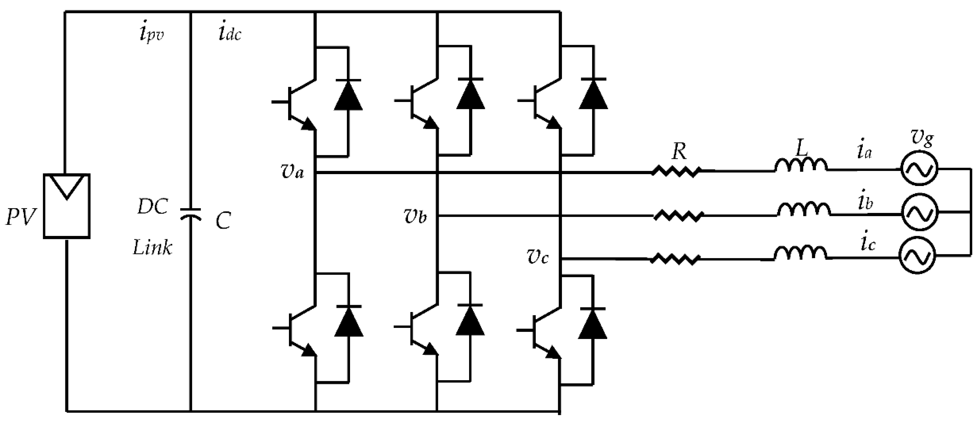
2. Grid-Connected Inverter System (GCIS)

2.1. GCIS Description

A GCIS is shown in Figure 1. The system contains a PV array, a DC link capacitor, a three-phase voltage source inverter (VSI), and a three-phase grid. The VSI facilitates the MPPT through regulation of the dc-link voltage, along with power transfer to the utility grid.

The output power of the PV system is a highly nonlinear and uncertain system. The PV output voltage corresponding to the maximum output power of the PV array varies with cell temperature and solar irradiation. The PV system should always be designed to operate at its maximum output power level. The MPPT technique is usually incorporated with the PV system to adjust the PV array output voltage to obtain the maximum available power at any change in solar irradiation or temperature of the cells. In addition, the MPPT scheme has the capability to release the dc-link voltage reference command [44]. Many MPPT techniques have been reported for PV systems, however, in practice, the most commonly used methods are perturb and observe (P&O) and the incremental conductance (IC) techniques [45].

2.2. MIMO Model of GCIS

The model of the GCIS shown in Figure 1 can be represented by

$$v_a{=Ri}_a+L\frac{{di}_a}{dt}{+v}_{ga}$$

(1)

$$v_b{=Ri}_b+L\frac{{di}_b}{dt}{+v}_{gb}$$

(2)

$$v_c{=Ri}_c+L\frac{{di}_c}{dt}{+v}_{gc}$$

(3)

where $v_{ga}{,v}_{gb}{,v}_{gc}$are the grid voltage components, $i_a{,i}_b{,i}_c$ are the grid current components, and $v_a,v_b,v_c$ are the inverter output voltage [46]. Park’s transformation is used to represent Equations (1)–(3) in the rotating $dq$ frame as

$$v_d{=v}_{gd}{+Ri}_d+L\frac{{di}_d}{dt}{+\omega Li}_q$$

(4)

$$v_q{=v}_{gq}{+Ri}_q+L\frac{{di}_q}{dt}{+\omega Li}_d$$

(5)

where $v_{gd}{,v}_{gq}$are the $dq$ grid voltage components, $i_d{,i}_q$are the $dq$ grid current components, and $v_d{,v}_q$ are the $dq$ inverter output voltage components. Upon neglecting the power loss in the inverter switches [46], the dc-input side connection with the ac-output side are given by

$$v_{gd}{i}_d{+v}_{gq}{i}_q{=v}_{dc}{i}_{dc}$$

(6)

$$C\frac{{dv}_{dc}}{dt}{=i}_{pv}{-i}_{dc}{=i}_{pv}-\frac{v_{gd}{i}_d{+v}_{gq}{i}_q}{v_{dc}}$$

(7)

where $v_{dc}$ and $i_{pv}$ are the PV output voltage and current respectively and $i_{dc}$ is the input current to the inverter.

Defining the state vector $x$ and the control input $u$ as

$$x=\left[\begin{array}{c}{x}_1\\ x_2\\ x_3\end{array}\right]=\left[\begin{array}{c}{i}_d\\ i_q\\ v_{dc}\end{array}\right]$$

(8)

$$u=\left[\begin{array}{c}{u}_1\\ { u}_2\end{array}\right]=\left[\begin{array}{c}{v}_d\\ { v}_q\end{array}\right]$$

(9)

Then, the state model of the GCIS can be formed as in Equation (10).

$$\dot{x}=\left[\begin{array}{c}-\frac{R}{L}{x}_1+\omega x_2-\frac{v_{gd}}{L}\\ -\frac{R}{L}{x}_2-\omega x_1-\frac{v_{gq}}{L}\\ \frac{i_{pv}}{C}-\frac{v_{gd}{x}_1+v_{gq}{x}_2}{C{x}_3}\end{array}\right]+\left[\begin{array}{cc}\frac{1}{L}& 0\\ 0& \frac{1}{L}\\ 0& 0\end{array}\right]u$$

(10)

The control objective is to regulate the power factor of the grid, through the q-component of the grid current, and the dc-input voltage $v_{dc}$. Therefore, the output vector of the system is considered as

$$y=\left[\begin{array}{c}{y}_1\\ y_2\end{array}\right]=\left[\begin{array}{c}{x}_2\\ x_3\end{array}\right]=\left[\begin{array}{c}{ i}_q\\ v_{\mathrm{dc}}\end{array}\right]$$

(11)

The Equations (10) and (11) can be written in the following general expression of the MIMO system

$$\dot{x}=f\left(x\right)+ g\left(x\right)u, y=h\left(x\right)$$

(12)

where $x$ is a $3\times 1$ state vector, $u$ is a $2\times 1$ control input vector, $y$ is a $2\times 1$ output vector, and $f\left(x\right)$ and $g\left(x\right)$ are defined by

$$f =\left[\begin{array}{c}{f}_1\\ f_2\\ f_3\end{array}\right]=\left[\begin{array}{c}-\frac{R}{L}{x}_1{+\omega x}_2-\frac{v_{gd}}{L}\\ -\frac{R}{L}{x}_2{-\omega x}_1-\frac{v_{gq}}{L}\\ \frac{i_{pv}}{C}-\frac{v_{gd}{x}_1{+v}_{gq}{x}_2}{{Cx}_3}\end{array}\right] , g =\left[\begin{array}{cc}\frac{1}{L}& 0\\ 0& \frac{1}{L}\\ 0& 0\end{array}\right]$$

(13)

The MIMO model of the GCIS in Equations (12) and (13) can be converted to a feedback linearizable form by using the input-output feedback linearization approach. In this approach, a nonlinear control signal is designed and used to convert the nonlinear system dynamics Equation (12) into decoupled linear subsystems. The feedback linearization for GCIS is presented next.

2.3. Input-Output Feedback Linearization of GCIS

In order to design a feedback linearization control, we used the notion of relative degree where each output is differentiated successively until one input $u_1$ or $u_2$ appears [47]. It can be shown that the relative degree $r_1$ for the first output $y_1$ is $r_1=1$ and the relative degree $r_2$ for the second output $y_2$ is $r_2=2$. The first derivative of $y_1$ and the second derivative of $y_2$ are given by Equations (14) and (15).

$${\dot{y}}_1=f_2+\frac{1}{L}{u}_2$$

(14)

$${\ddot{y}}_2={\dot{f}}_3=\frac{1}{C}\frac{d{i}_{pv}}{dt}-\frac{1}{C.x_3}\left[v_{gd}\left(f_1+\frac{1}{L}{u}_1\right)+v_{gq}\left(f_2+\frac{1}{L}{u}_2\right)\right]+\frac{\left(v_{gd}{x}_1+v_{gq}{x}_2\right)}{C{x}_3^2}{f}_3$$

(15)

Equations (14) and (15) can be cast in the following matrix form

$$\left[\begin{array}{l}{\dot{y}}_1\hfill \\ {\ddot{y}}_2\hfill \end{array}\right]=\alpha (x)+\beta (x)\left[\begin{array}{l}{u}_1\hfill \\ u_2\hfill \end{array}\right]$$

(16)

where

$$\alpha \left(x\right) =\left[\begin{array}{c}{f}_2\\ m-\frac{1}{{Cx}_3}\left(v_{gd}{f}_1{+v}_{gq}{f}_2\right)+\frac{\left(v_{gd}{x}_1{+v}_{gq}{x}_2\right)}{{Cx}_3^2}{f}_3\end{array}\right]$$

(17)

$$\beta \left(x\right)=\left[\begin{array}{cc}0& \frac{1}{L}\\ -\frac{v_{gd}}{{LCx}_3}& -\frac{v_{gq}}{{LCx}_3}\end{array}\right]$$

(18)

and $m=\frac{1}{C}\frac{{di}_{pv}}{dt}$.

The control law in Equation (19) when used in Equation (16) yields to the linear input-output relation in Equation (20)

$$\left[\begin{array}{c}{u}_1\\ u_2\end{array}\right]{=\beta }^{-1}\left(x\right)\left[\begin{array}{c}{v}_1{-\alpha }_1\\ v_2{-\alpha }_2\end{array}\right]$$

(19)

$$\left[\begin{array}{l}{\dot{y}}_1\hfill \\ {\ddot{y}}_2\hfill \end{array}\right]=\left[\begin{array}{l}{v}_1\hfill \\ v_2\hfill \end{array}\right]$$

(20)

where${ v}_1$ and $v_2$ are external signals that can be chosen in a way to ensure asymptotic tracking of the outputs $y_1$ and $y_2$ to their references $y_{ref1}{=i}_{qref}$ and $y_{ref2}{=v}_{dcref}$. Defining the tracking errors $e_1=\left(y_{ref1}{- y}_1\right)$ and $e_2=\left(y_{ref2}{- y}_2\right)$, the signals $v_1$ and $v_2$ can be selected as

$$v_1=k_{01}{e}_1+{\dot{y}}_{ref1}$$

(21)

$$v_2=k_{02}{e}_2+k_{12}{\dot{e}}_2+{\ddot{y}}_{ref2}$$

(22)

Now, substituting Equations (21) and (22) into Equation (20), we obtain the following tracking errors dynamics:

$${\dot{e}}_1+k_{01}{e}_1=0$$

(23)

$${\ddot{e}}_2+k_{12}{\dot{e}}_2+k_{02}{e}_2=0$$

(24)

The coefficients${ k}_{01}$, $k_{02}$, and $k_{12}$ are design parameters selected such that the characteristic polynomials of Equations (23) and (24) are Hurwitz and hence ensuring that the tracking errors $e_1$ and $e_2$converge to zero asymptotically [47]. It is worth mentioning that the control law given in Equation (19) is implementable since the matrix $\beta \left(x\right)$ is non-singular, provided that $e_d\ne 0$ (which is the case for GCIS).

A main disadvantage of the control law in Equation (19) is that the exact values of the system parameters involved in $\alpha \left(x\right)$ and $\beta \left(x\right)$ should be known and any change in the parameters affects the output of the controller. In practice, the parameters of the GCIS may be unknown or imprecise and the uncertainty in these parameters is inevitable. To overcome this drawback, the universal approximation capability of the fuzzy systems is used to approximate the nonlinear functions $\alpha \left(x\right)$ and $\beta \left(x\right)$. In the next section, the proposed adaptive fuzzy controller for GCIS is presented.

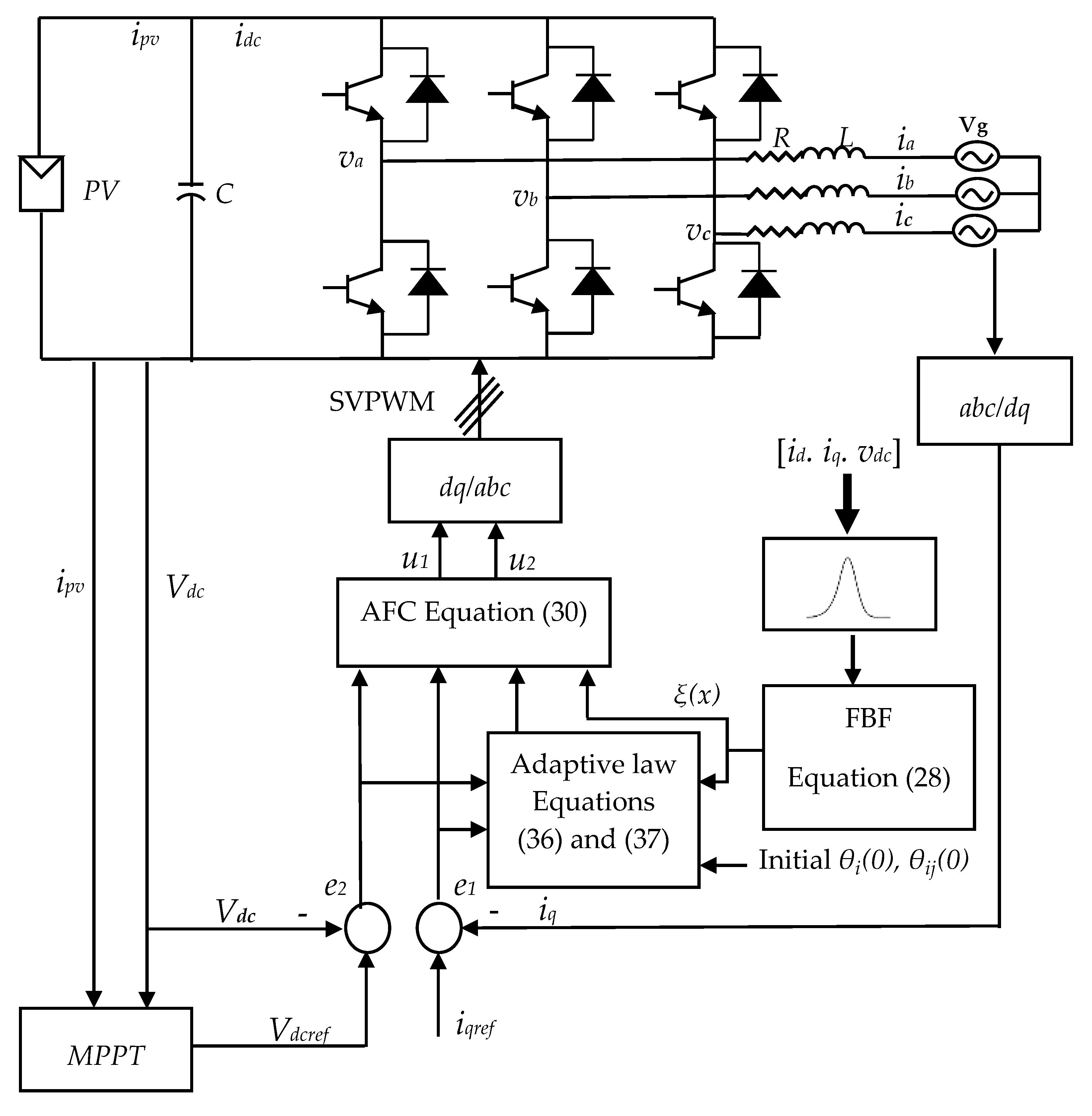
3. The Proposed Controller

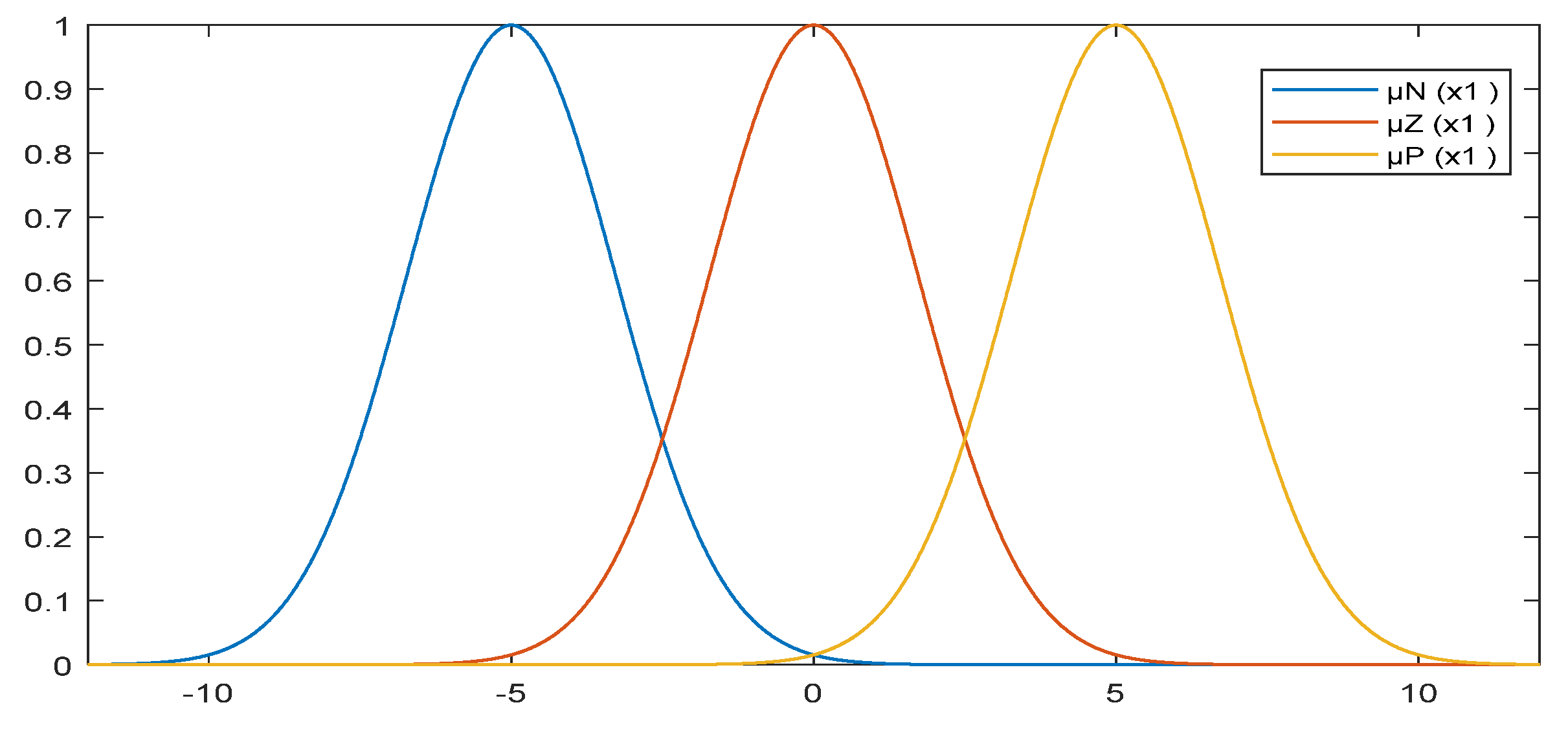
3.1. Adaptive Fuzzy Approximation Controller for GCIS

In this section, the proposed controller is developed using the Equation (12) which is a square MIMO nonlinear system. The input-output feedback linearization given in Equation (16) with $r_1=1$ and $r_2=2$ can be written in the form

$$y^{\left(r\right)}=\alpha \left(x\right)+\beta \left(x\right)u$$

(25)

where $y^{\left(r\right)}=\left[\begin{array}{c}{y}_1^{{(r}_1)}\\ y_2^{{(r}_2)}\end{array}\right]=\left[\begin{array}{c}\dot{y_1}\\ \ddot{y_2}\end{array}\right], u=\left[\begin{array}{c}{u}_1\\ u_2\end{array}\right]$, $\alpha \left(x\right)$ and $\beta \left(x\right)$ are as given in Equations (17) and (18), and their entries are in general nonlinear functions with imprecise parameters.

Approximations of the nonlinear functions $\alpha \left(x\right)$ and $\beta \left(x\right)$ were generated using a fuzzy logic system with singleton fuzzifier, product inference rule, and weighted average defuzzifier. To construct these estimates, the notion of the fuzzy basis function (FBF) expansion $\xi \left(x\right)$ was used [37]. The fuzzy estimates ${\widehat{a}}_i(x)$ and ${\widehat{\beta }}_{ij}(x)$ of the nonlinear functions ${\alpha }_i\left(x\right)$ and ${ \beta }_{ij}\left(x\right), i=1,2 \mathrm{and} j=1,2$ were determined as

$${\widehat{a}}_i(x)={{\theta }_i}^T\xi (x)$$

(26)

$${\widehat{\beta }}_{ij}(x)={{\theta }_{ij}}^T\xi (x)$$

(27)

where ${\theta }_i\in R^{M\times 1}$ and ${\theta }_{\mathrm{ij}}\in R^{M\times 1}$ represent vectors of adjustable parameters and $\xi \left(x\right)\in R^{M\times 1}$ represents the vector of FBFs. The FBF was generated using the weighted-average defuzzifier [48].

$${\xi }_i\left(x\right)=\frac{{\prod }_{i=1}^n{x}_i{ \mu }_{il}{(x}_i)}{{\sum }_{l=1}^M\left({\prod }_{i=1}^n{\mu }_{il}\left(x_i\right)\right)}$$

(28)

where$n$ is the number of states, ${\mu }_{il}{(x}_i)$ is the membership function of the $i^{th}$ state $x_i$ in the $l^{th}$ rule, and $M$ is the number of If-Then rules.

Upon replacing $\alpha \left(x\right)$ and $\beta \left(x\right)$ in Equation (25) by their corresponding fuzzy estimates Equations (26) and (27), we get

$$y^{(r)}=\widehat{\alpha }(x)+\widehat{\beta }(x)u$$

(29)

where $\widehat{\alpha }(x)=\left[\begin{array}{c}{\widehat{\alpha }}_1\\ {\widehat{\alpha }}_2\end{array}\right]$ and $\widehat{\beta }(x)=\left[\begin{array}{cc}{\widehat{\beta }}_{11}& {\widehat{\beta }}_{12}\\ {\widehat{\beta }}_{21}& {\widehat{\beta }}_{22}\end{array}\right]$.

Therefore, the AFC can be written in terms of the fuzzy estimates Equations (26) and (27) as

$$u={\widehat{\beta }}^{-1}(x)\left(y_{ref}^{(r)}+K\underset{¯}{e}-\widehat{\alpha }(x)\right)$$

(30)

where $y_{ref}^{\left(r\right)}={\left[{ y}_{ref1}^{\left(r_1\right)}{ y}_{ref2}^{\left(r_2\right)}\right]}^T$, $K=diag\left[k_1{ k}_2 \right]$, $\underset{¯}{e} = {\left[{\underset{¯}{e}}_1 {\underset{¯}{e}}_2\right]}^T$, $k_1{ = k}_{01}$, $k_2{ = [k}_{02}{ k}_{12}]$, ${\underset{¯}{e}}_1{ = e}_1$, ${\underset{¯}{e}}_2{ = [e}_2{ \dot{e}}_{2 }]$, and $e_i = y_{refi}{-y}_i, i = 1,2.$ It is worth mentioning that the implementation of the proposed AFC given in Equation (30) needs only the fuzzy estimates $\widehat{\alpha }(x)$ , $\widehat{\beta }(x)$ , the derivatives of the reference signal $y_{ref}^{\left(r\right)},$and the tracking error $\underset{¯}{e}$.

3.2. Closed-Loop Stability

In this section, we show the boundedness of both the tracking error and the adjustable parameters via the Lyapunov function analysis. Equation (30) can be rewritten as

$$\widehat{\beta }(x)u=\left(y_{ref}^{(r)}-y^{(r)}\right)+K\underset{\_}{e}+y^{(r)}-\widehat{\alpha }(x)$$

(31)

Using Equation (25) in Equation (31) to obtain the following error equation in terms of the fuzzy approximation errors, it becomes

$$\left[\begin{array}{c}{e}_1^{\left(r_1\right)}\\ e_2^{\left(r_2\right)}\end{array}\right]=\left(y_{ref}^{(r)}-y^{(r)}\right)=-K\underset{¯}{e}+(\widehat{\alpha }(x)-\alpha (x))+(\widehat{\beta }(x)-\beta (x))u$$

(32)

From Equation (32), the error equation for the $i^{th}$ output becomes

$$e_i^{r_i}=-k_i{\underset{\_}{e}}_i+\Delta {\alpha }_i(x)+{\displaystyle \sum _{j=1}^p\Delta }{\beta }_{ij}(x)u_j$$

(33)

where $\Delta {\alpha }_i(x)={\widehat{\alpha }}_i(x)-{\alpha }_i(x)$ and $\Delta {\beta }_{ij}(x)={\widehat{\beta }}_{ij}(x)-{\beta }_{ij}(x)$ are the fuzzy approximation errors.

In state-variable form, the error equation of the $i^{th}$ output Equation (33) takes the form

$${\dot{\underset{¯}{e}}}_i=A_i{\underset{¯}{e}}_i+[\Delta {\alpha }_i(x)+{\displaystyle \sum _{j=1}^{p=2}\Delta }{\beta }_{ij}(x)u_j]b_i$$

(34)

where $A_i$ and $b_i$ are given by

$$\{\begin{array}{c}{A}_1{=-k}_{01}{, b}_1=1\\ A_2=\left[\begin{array}{cc}0& 1\\ {-k}_{12}& {-k}_{02}\end{array}\right]{, b}_2=\left[\begin{array}{c}0\\ 1\end{array}\right]\end{array}$$

(35)

Theorem 1.

The closed-loop tracking error $\underset{¯}{e} = {\left[{\underset{¯}{e}}_1 {\underset{¯}{e}}_2\right]}^T$ is globally ultimately bounded if the updating laws of the parameter vectors${\theta }_i\in R^{M\times 1}$and${\theta }_{ij}\in R^{M\times 1}$are chosen as in Equations (36) and (37):

$${\dot{\theta }}_i=-{\gamma }_i{{\underset{¯}{e}}_i}^T{P}_i{b}_i\xi (x)$$

(36)

$${\dot{\theta }}_{ij}=-{\gamma }_{ij}{{\underset{¯}{e}}_i}^T{P}_i{b}_i\xi (x)u_j$$

(37)

where${\gamma }_i$and${\gamma }_{ij}$are design parameters and$P_i$is a unique positive definite matrix solution of the Lyapunov Equation (38) with arbitrary positive definite matrix$Q_i$

$$A_i{}^T{P}_i{+P}_i{A}_i{=-Q}_i$$

(38)

Proof. 

Define the minimum fuzzy approximation error $w_i$ in terms of the optimal values of adjustable parameters ${\theta }_i^{\ast }$ and ${\theta }_{ij}^{\ast }$ as

$$w_i=\left[{\widehat{\alpha }}_i\left(x\mid {\theta }_i^{\ast }\right)-{\alpha }_i(x)\right]+{\displaystyle \sum _{j=1}^{p=2}\left[{\widehat{\beta }}_{ij}\left(x\mid {\theta }_{ij}^{\ast }\right)-{\beta }_{ij}(x)\right]}{u}_j$$

(39)

Add and subtract the terms ${\widehat{\alpha }}_i\left(x\mid {\theta }_i^{\ast }\right)$ and ${\widehat{\beta }}_{ij}(x\mid {\theta }_{ij}^{\ast })$ to Equation (34) and then use the definition given in Equation (39) to obtain the following error equation

$${\dot{\underset{¯}{e}}}_i=A_i{\underset{¯}{e}}_i+b_i[w_i+{\phi }_{{\alpha }_i}^T\xi (x)+{\displaystyle \sum _{j=1}^{p=2}{\phi }_{{\beta }_{ij}}^T}\xi (x)u_j]$$

(40)

where ${\phi }_{{\alpha }_i}{=(\theta }_i{-\theta }_i^{*})$ and ${\phi }_{{\beta }_{ij}}=\left({\theta }_{ij}{-\theta }_{ij}^{*}\right)$ are the parameter errors. Note that the derivatives of these parameter errors are given by:

$${\dot{\phi }}_{{\alpha }_i}={\dot{\theta }}_i$$

(41)

$${\dot{\phi }}_{{\beta }_{ij}}={\dot{\theta }}_{ij}$$

(42)

The following positive Lyapunov function is formulated as a quadratic function of the error involved, namely the tracking error (34) and the parameter error (41) and (42):

$$V_i=\frac{1}{2}{\underset{¯}{e}}_i^T{P}_i{\underset{¯}{e}}_i+\frac{1}{2{\gamma }_i}{\phi }_{{\alpha }_i}^T{\phi }_{{\alpha }_i}+{\displaystyle \sum _{j=1}^{p=2}\frac{1}{2{\gamma }_{ij}}}{\phi }_{{\beta }_{ij}}^T{\phi }_{{\beta }_{ij}}$$

(43)

The time derivative of Equation (43) along the trajectories Equations (40)–(42) is found as:

$${\dot{V}}_i=-\frac{1}{2}{\underset{¯}{e}}_i^T{Q}_i{\underset{¯}{e}}_i+\frac{1}{{\gamma }_i}{\phi }_{{\alpha }_i}^T\left({\dot{\theta }}_i+{\gamma }_i{{\underset{¯}{e}}_i}^T{P}_i{b}_i\xi (x)\right)+\left(\frac{1}{{\gamma }_{ij}}{\displaystyle \sum _{j=1}^{p=2}{\phi }_{{\beta }_{ij}}^T}{\dot{\theta }}_{ij}+{{\underset{¯}{e}}_i}^T{P}_i{b}_i{\displaystyle \sum _{j=1}^{p=2}{\phi }_{{\beta }_{ij}}^T}\xi (x)u_j\right)+{{\underset{¯}{e}}_i}^T{P}_i{b}_i{w}_i$$

(44)

Now, substituting the parameters’ updating laws in Equations (36) and (37) in Equation (44) to get:

$${\dot{V}}_i=-\frac{1}{2}{\underset{¯}{e}}_i^T{Q}_i{\underset{¯}{e}}_i+{\underset{¯}{e}}_i{}^T{P}_i{b}_i{w}_i$$

(45)

Provided that $\left|\right|{\underset{¯}{e}}_i\left|\right|\ge \frac{4{\sigma }_i{\lambda }_{max}\left(P_i\right)}{{\beta }_i{\lambda }_{min}\left(Q_i\right)}=r_i$ , it is straightforward to write Equation (45) in the form

$${\dot{V}}_i\le -\frac{1}{2}\left(1-{\beta }_i\right){\lambda }_{min}\left(Q_i\right){\left|\right|{\underset{¯}{e}}_i\left|\right|}^2$$

(46)

where ${0 < \beta }_i < 1$, ${\sigma }_i>0$, such that $\left|\right|{\underset{¯}{w}}_i\left|\right|\le {\sigma }_i$, ${\lambda }_{min}\left(Q_i\right)$ and ${\lambda }_{max}\left(P_i\right)$ are the minimum and maximum eigenvalues of the indicated matrices and $\left|\right|.\left|\right|$ stands for the Euclidean norm. From the positive definiteness of Equation (43) and the negative definiteness of Equation (46), we conclude that the tracking error is globally ultimately bounded with bound ${\mu }_{bi}{=r}_i\sqrt{\frac{{\lambda }_{max}\left(P_i\right)}{{\lambda }_{min}\left(P_i\right)}}$ [47]. In Equation (43), the Lyapunov function is quadratic; the non-quadratic Lyapunov function can also be used in adaptive schemes for better performance [49]. □

4. Implementation of the Proposed Adaptive Fuzzy Controller for GCIS

In order to implement the proposed AFC based on feedback linearization given by Equations (26), (27), (32), (36), and (37), fuzzy sets $F_k^i$ have to be selected where $i=1, 2, \dots N$, $N$ is the number of the fuzzy sets and $k=1, 2, 3$. The fuzzy sets are utilized to determine the vector of FBFs given in Equation (28). To this end, three Gaussian fuzzy sets, namely Negative (N), Zero (Z), and Positive (P) are used to generate the FBFs for each state of the system. These fuzzy sets are characterized by the membership functions. The general form of the membership functions of Gaussian type is given by

$${\mu }_{F_k^i}\left(x_k\right)=exp\left(-\frac{{\left(x_k-{\overline{x}}_k^i\right)}^2}{{\sigma }_k^i}\right)$$

(47)

where ${\overline{x}}_k^i$ and ${\sigma }_k^i$ are the center and the width of the $i^{th}$ fuzzy set $F_k^i$.

The block diagram of the proposed controller is shown in Figure 2. It can be seen in the block diagram that the grid voltage and current are transformed into a dq frame from an abc frame. The control laws in Equations (36) and (37) were used to estimate the unknown parameters of GCIS, where the calculation initially started from chosen initial values of ${\theta }_i$ and ${\theta }_{ij}$. Then, AFC low in Equation (30) was applied to generate the control signals. The PWM was generated by applying space vector pulse width modulation (SVPWM) to drive the inverter. Note that the signal $V_{dcref}$ is released from the MPPT algorithm.

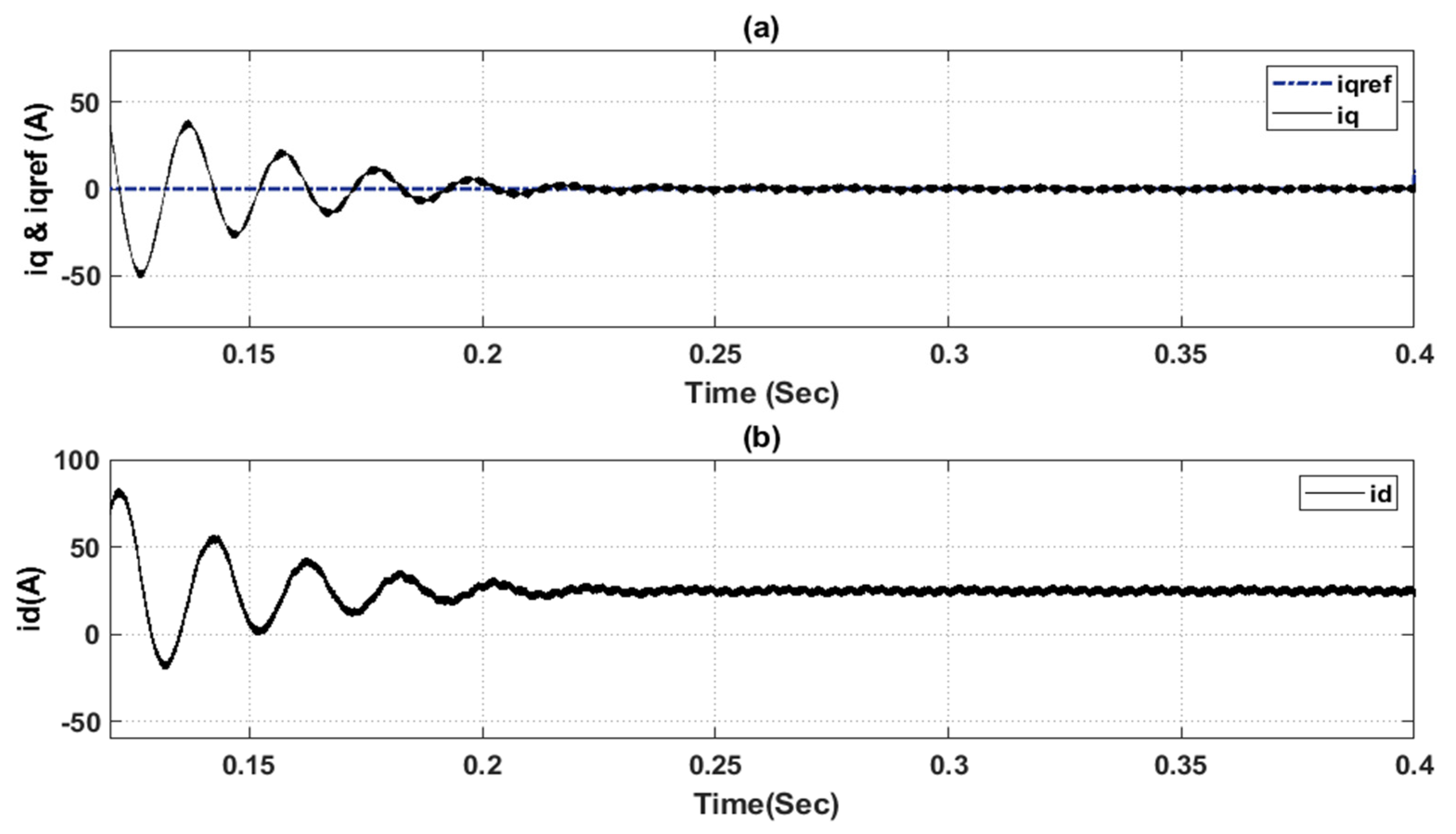
5. Simulation Cases and Results

To examine the effectiveness of the proposed controller performance, the proposed AFC was implemented and tested in the MATLAB/SIMULINK [50] environment for a GCIS having the parameters as listed in

Table 1. System parameters.

Parameter	Value
Grid Voltage rms	120 V
Inductance L Resistor R	2 mH 0.1 Ω
Grid Frequency	50 Hz
DC link capacitor	2200 µF
PV array voltage Vdc	540 V
PV array current Ipv	3.46 A

. The other design parameters were selected as $k_{01}=10$, $k_{02}{=k}_{12}=\mathrm{10,000}$,${ \gamma }_1=40$,${ \gamma }_2=0.01$,${ \gamma }_{11}=0.01$,${ \gamma }_{12}=0.1$, ${\gamma }_{21}=0.1$, and${ \gamma }_{22}=1$. The selected positive definite matrices $Q_i$ and the unique positive definite matrix solution $P_i, i=1,2$that appeared in Lyapunov Equation (38) are given by

$$Q_1{=100, Q}_2=\left[\begin{array}{cc}2000& 0\\ 0& 1\end{array}\right]{, P}_1{=5, P}_2=\left[\begin{array}{cc}1000.6& 0.1\\ 0.1& 0.00006\end{array}\right]$$

For each state of the system, the parameters of the Gaussian membership functions given in Equation (47) are listed in

Table 2. Parameters of the Gaussian membership functions.

$\mathbf{State}\downarrow$	$\mathbf{Fuzzy} \mathbf{Set}\to$	N	Z	P
$x_1$		$$\begin{gathered} {\overline{x}}_1^N=-5 \\ {\sigma }_1^N=6 \end{gathered}$$	$$\begin{gathered} {\overline{x}}_1^Z=0 \\ {\sigma }_1^Z=6 \end{gathered}$$	$$\begin{gathered} {\overline{x}}_1^P=5 \\ {\sigma }_1^P=6 \end{gathered}$$
$x_2$		$$\begin{gathered} {\overline{x}}_2^N=-0.1 \\ {\sigma }_2^N=0.005 \end{gathered}$$	$$\begin{gathered} {\overline{x}}_2^Z=0 \\ {\sigma }_2^Z=0.005 \end{gathered}$$	$$\begin{gathered} {\overline{x}}_2^P=0.1 \\ {\sigma }_2^P=0.005 \end{gathered}$$
$x_3$		$$\begin{gathered} {\overline{x}}_3^N=525 \\ {\sigma }_3^N=100 \end{gathered}$$	$$\begin{gathered} {\overline{x}}_3^Z=550 \\ {\sigma }_3^Z=100 \end{gathered}$$	$$\begin{gathered} {\overline{x}}_3^P=575 \\ {\sigma }_3^P=100 \end{gathered}$$

. The membership functions for the state $x_1$ are shown in Figure 3, as an example for states membership functions.

The proposed AFC was studied under different operating cases as unity power factor tracking, tracking of power factor changes, and robust tracking. Smooth reference values were used for all simulation cases.

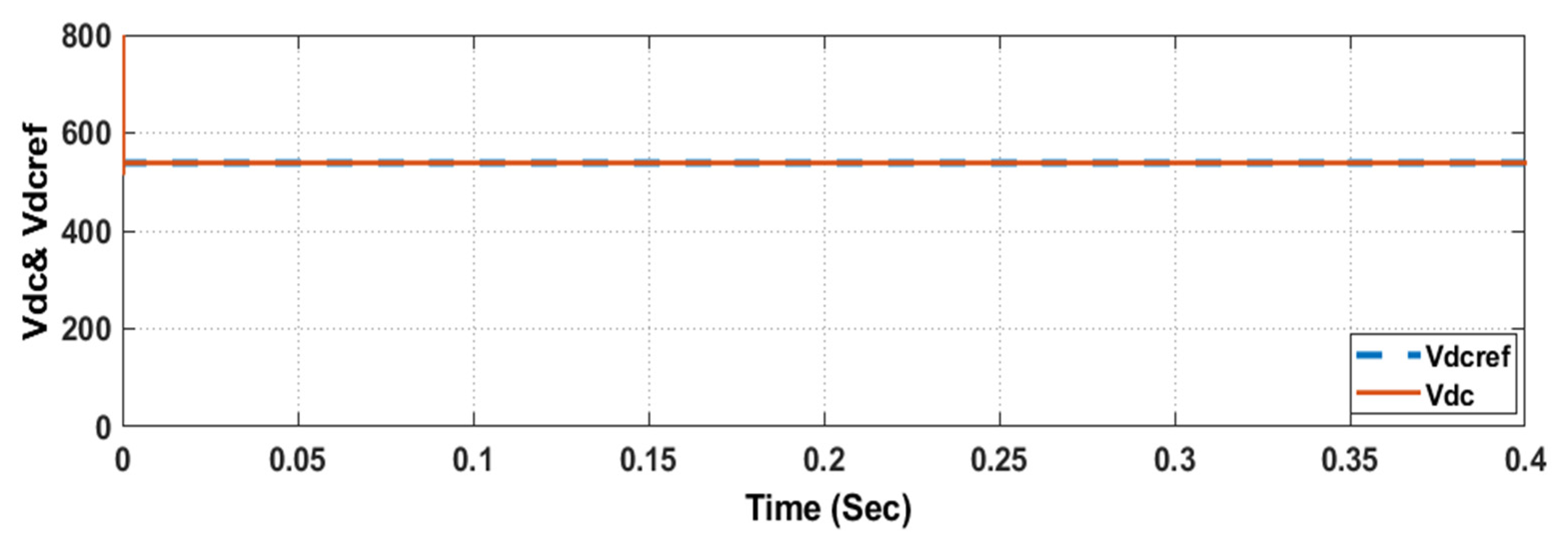
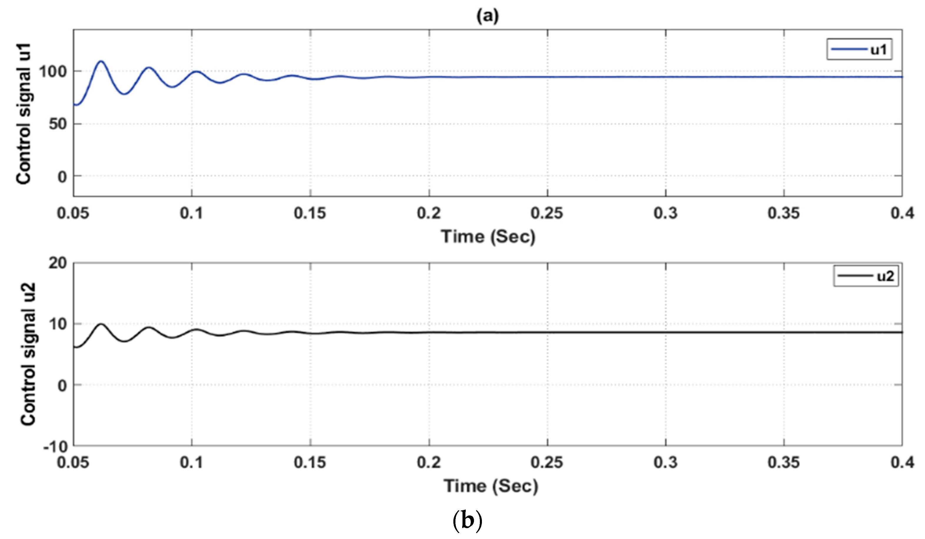
5.1. Case I: Unity Power Factor Tracking

In this case, simulation was carried out by selecting the reference grid current components as $i_{qref }= 0.0$ A, which corresponds to unity power factor. The output voltage and current are shown in Figure 4. The figure clearly shows that the grid current is in phase with grid voltage, which indicates unity PF operation. Figure 5a,b depicts the reactive $i_q$ and active $i_d$ current tracking output of the proposed controller. The DC voltage and reference voltage are shown in Figure 6. The control signal $u_1$ and $u_2$ are shown in Figure 7a,b, from which it can be noticed that they are bounded. From the obtained result in case of the unity power factor, it can be stated that the proposed controller provides excellent tracking performance with bounded tracking error and bounded control signals.

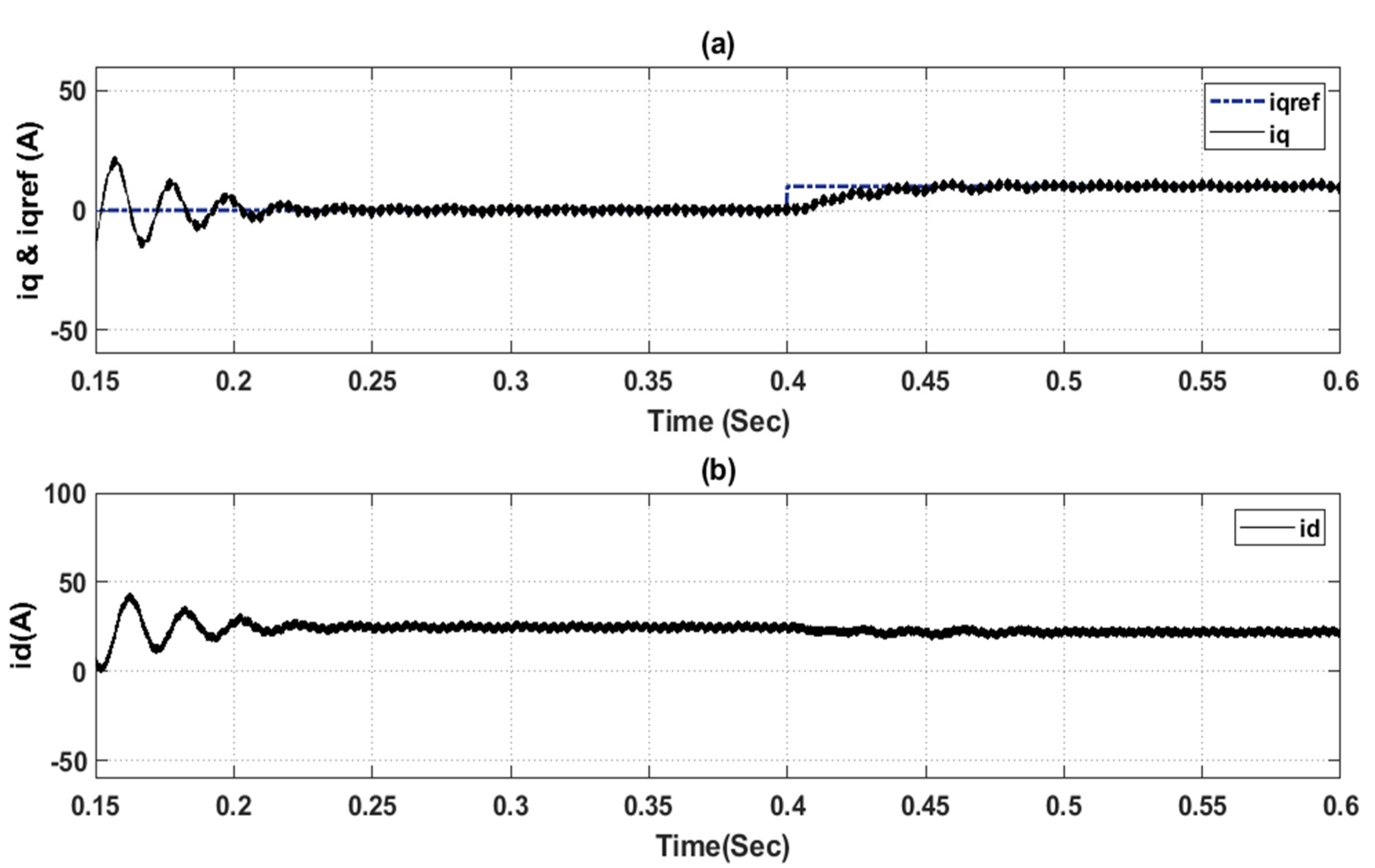
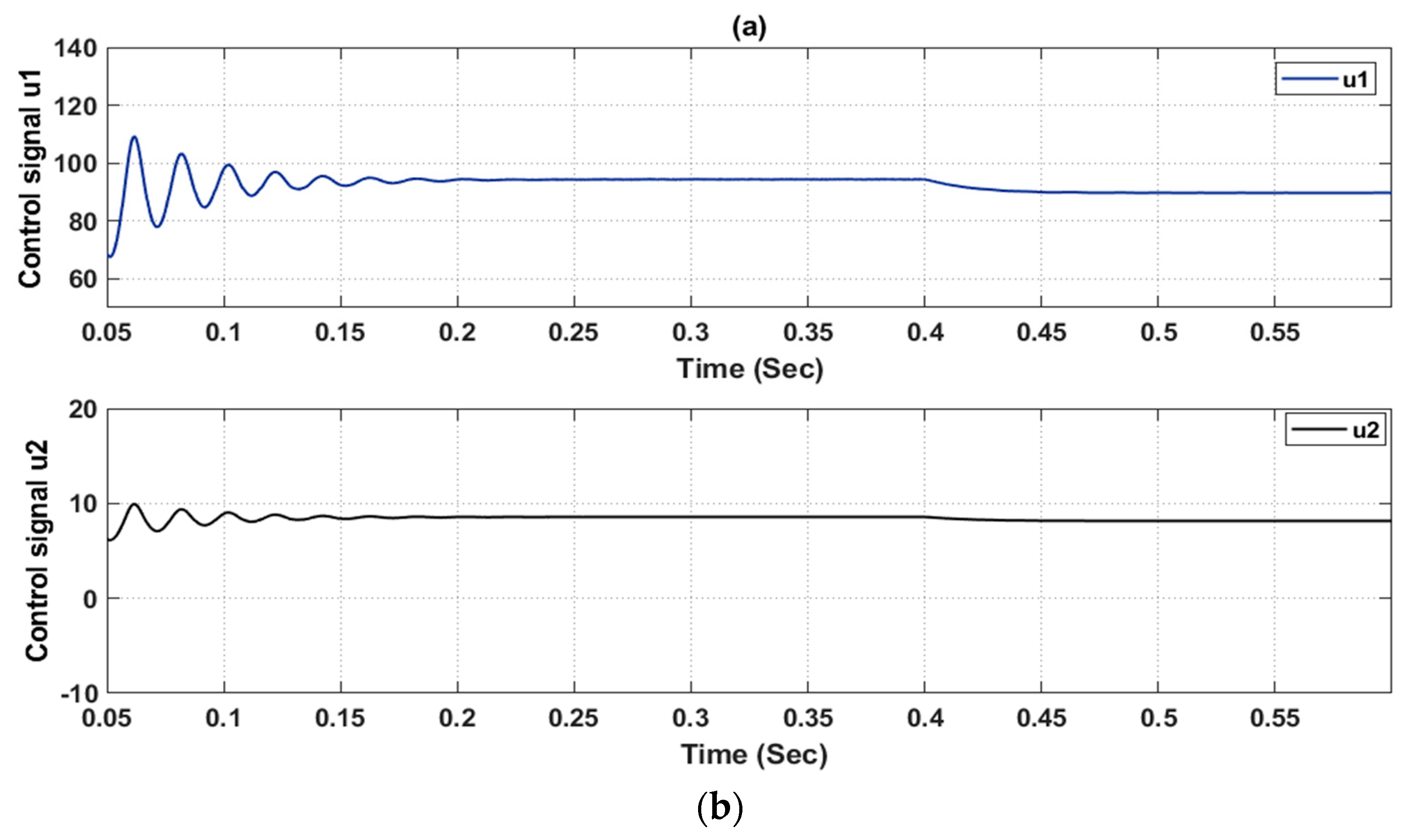
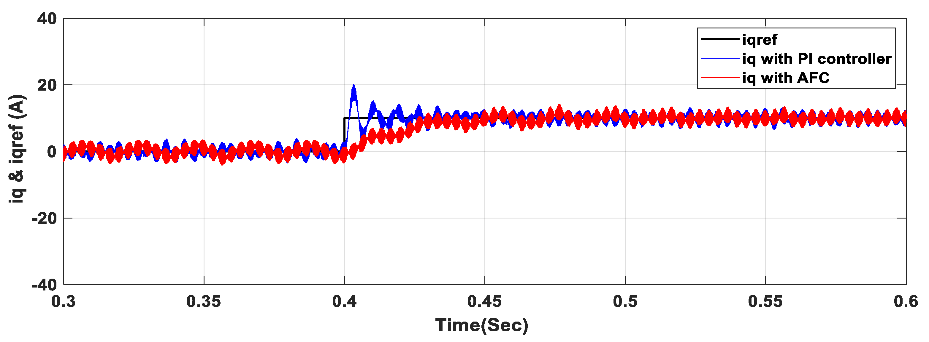
5.2. Case II: Tracking of Power Factor Changes

In this case study, the performance of the proposed AFC was tested for power factor tracking. At the start, the system was assumed to operate at unity power factor with $i_{qref}=0$, then a step change of 10 A in $i_{qref}$ at 0.4 s was applied. This change in $i_{qref}$corresponded to a change in the power factor to 0.937. Figure 8a,b display the effect of changes in $i_{qref}$, $i_q,$ and $i_d$. The results demonstrate that $i_q$ reaches its new reference quickly. Hence, the obtained results clearly prove that the proposed AFC has the ability to track power factor changes. The output voltage and current are shown in Figure 9. A phase shift can be noticed between current and voltage after t = 0.4 s, confirming the tracking of the desired power factor. The active and reactive power delivered by the inverter to the grid are shown in Figure 10a,b, confirming the proposed controller tracking ability. The bounded control signals $u_1{=v}_d$ and $u_2{=v}_q$ are shown in Figure 11a,b.

To evaluate the effectiveness of AFC, the performance of the proposed controller was compared with the PI controller as in [51]. The comparison was conducted for power factor change tracking case by applying a step change of 10 A in $i_{qref}$ at 0.4 s. Figure 12 demonstrates the performance of the proposed AFC and PI controller. The result illustrates that the tracking between $i_q$ and $i_{qref}$ after the step change occurs has less fluctuations and overshooting in case of proposed AFC in comparison to the PI controller. Moreover, a comparison between the performance of the proposed controller, the PI controller, and the TSKPFNN controller presented in [35] is shown in

Table 3. Comparison between the performance of the proposed controller, PI, and TSKPFNN controllers.

Controller	Max Overshoot %	Settling Time (S)
PI controller	75	0.04
TSKPFNN controller	12.24	0.3
Proposed AFC	0.0	0.035

. From the illustrated results in Table 3, it can be said that the performance of proposed AFC is better and exceeds the PI controller and TSKPFNN controller performances.

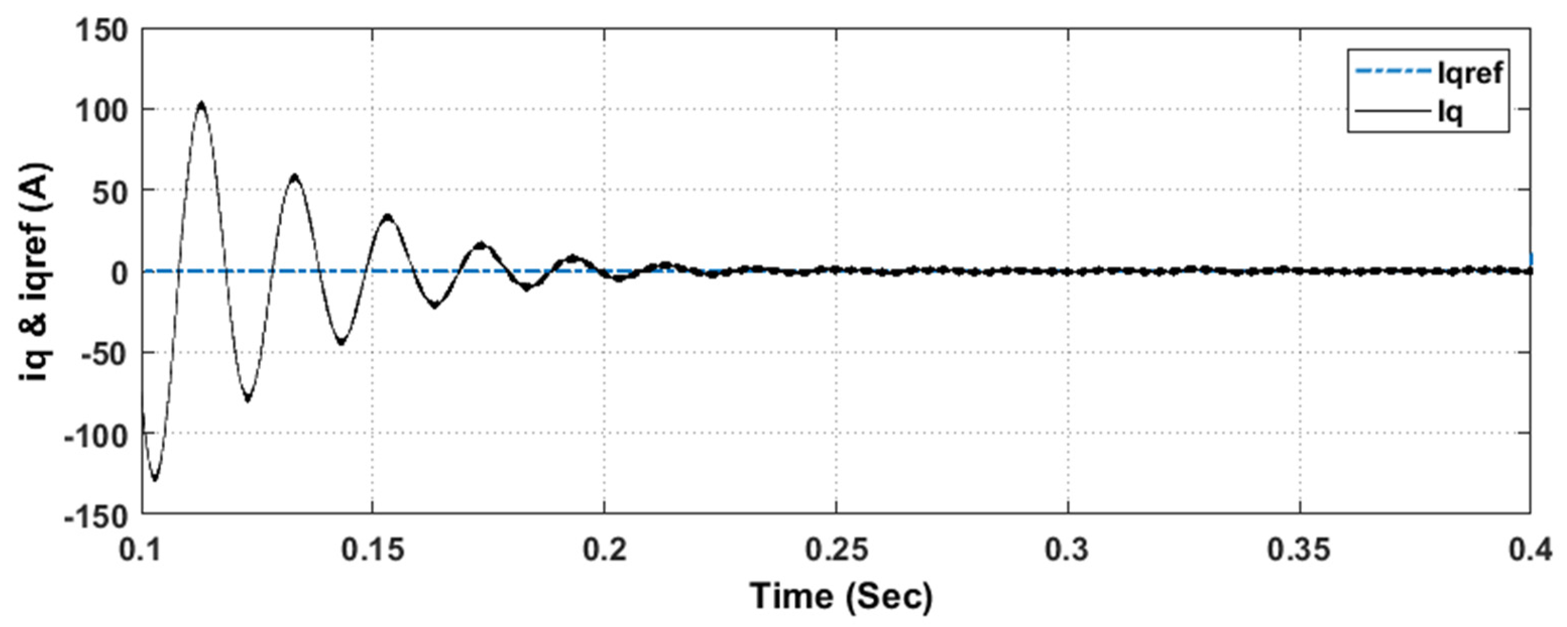
5.3. Case III: Robust Tracking

In certain cases, the parameters used in the GCIS are either time-varying or not precisely defined, so there are often parametric uncertainties where the filters connected to the grid inductance value change over time, affected by the impedance value of the grid which varies depending on the grid structure and conditions leading to resonance and instability problems. In addition, due to changes in ambient operating temperature or changes in applied voltage and frequency, DC Link capacitance values can change.

In this simulation case, the robustness of the proposed AFC was tested for GCIS parameter variations. Simulations were carried out for different percentages of variations in filter inductor $L$ and dc-link capacitor $C$. Grid reactive current component $i_q$, with 10% variations in filter inductor $L,$ is shown in Figure 13. Figure 14 illustrates the bounded control signals of the proposed controller with the same variation in $L$. The obtained results illustrate the robustness of the AFC with filter inductor increase.

To study the robustness of the proposed AFC for variations dc-link capacitor $C$, simulations were carried out for 30% increase and carried again for 20% decrease in $C$. The performance of the GCIS with proposed AFC with applied variations is shown in Figure 15, Figure 16, Figure 17 and Figure 18, where Figure 15a,b displays $i_q$ and $i_d$ with 30% increase in C. Grid voltage and current with the same increase in C are shown in Figure 16. For the case of the 20% decrease in C, Figure 17 illustrates the bounded control signals; tracking between $i_q$ and $i_{qref}$, is shown in Figure 18. The obtained simulation results with variations in C prove the robustness of the controller. Furthermore, Figure 19 displays the performance of the proposed controller for variation in the inductor and capacitor at the same time with 10% increase in $L$ and 30% increase in $C$.

From all conducted simulation results for parameter uncertainties, the performance of the GCIS proves that the proposed AFC is capable to cope with the uncertainty of the GCIS parameters and achieve the desired tracking performance.

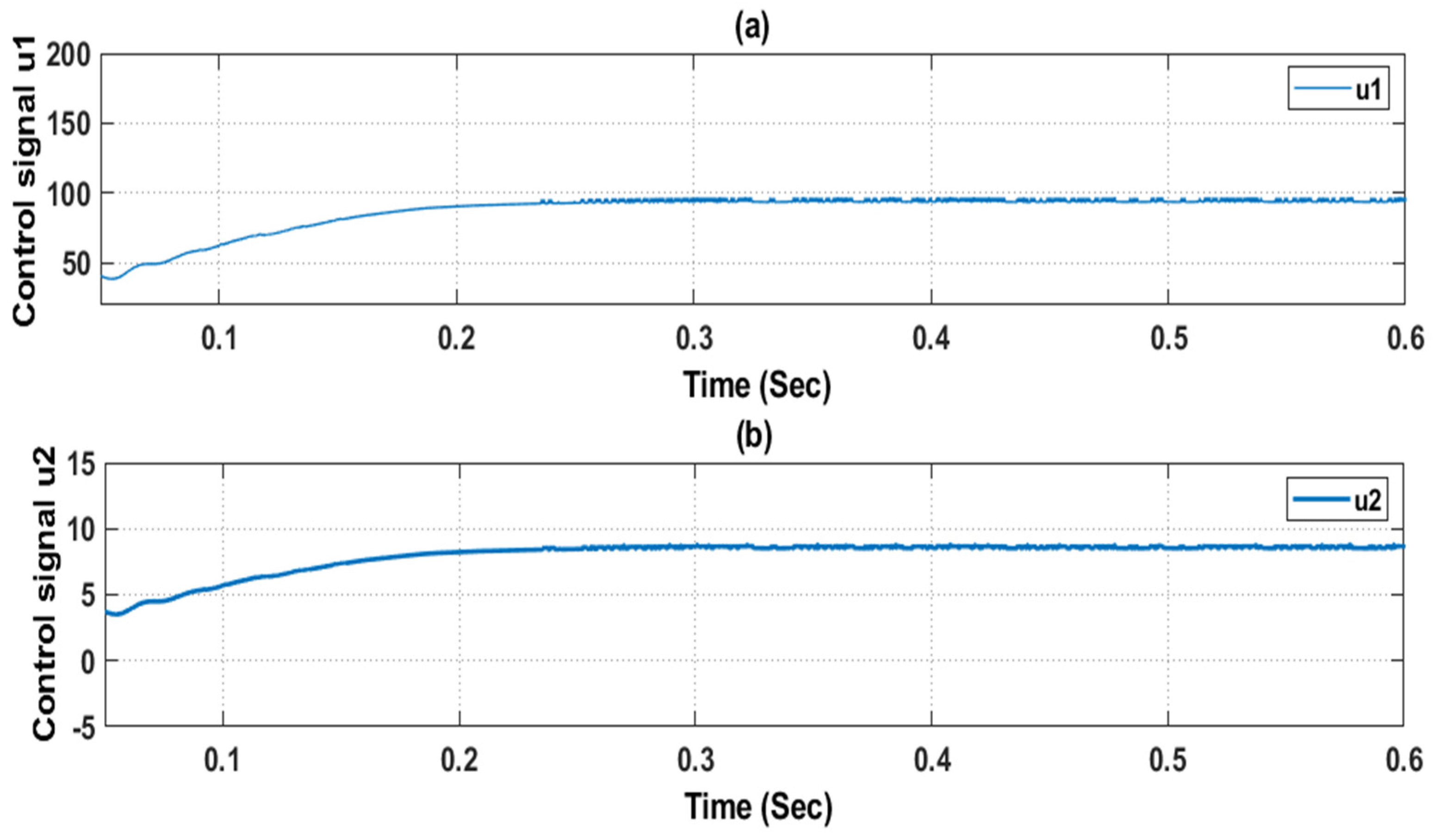
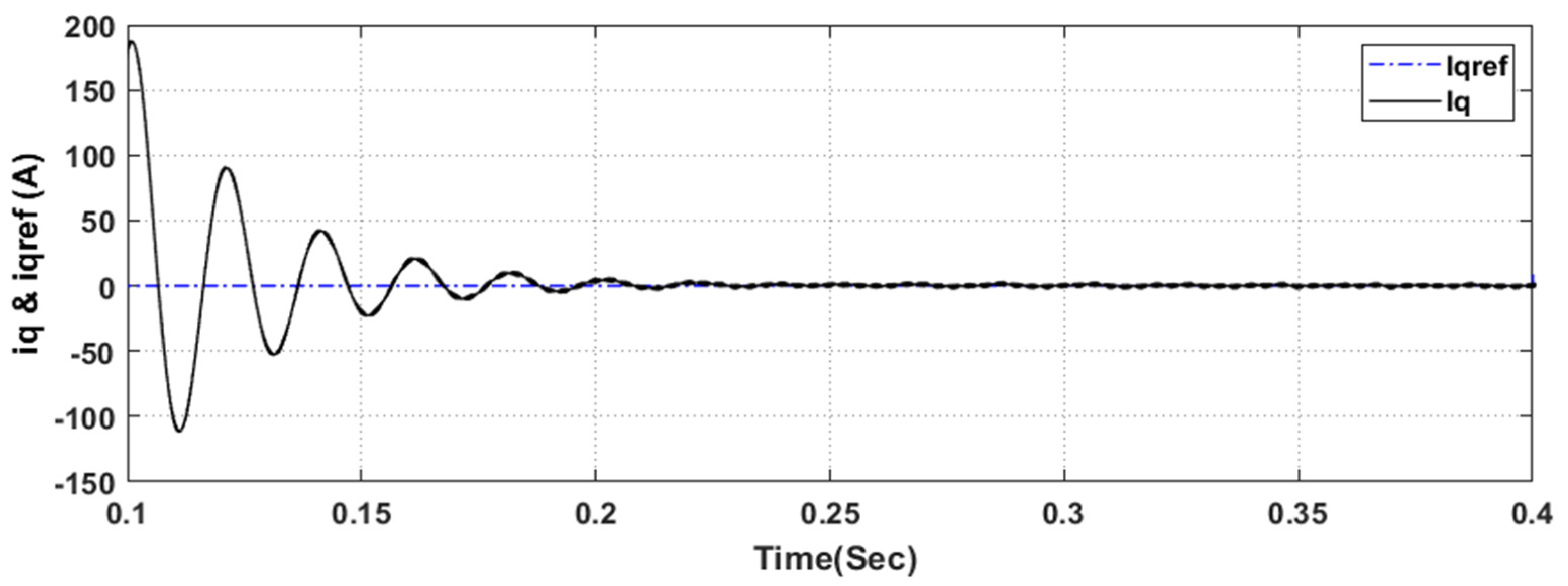
5.4. Case IV: Tracking in the Presence of Model Uncertainity

The proposed AFC given in (30) can achieve tracking in presence of modelling uncertainties that are inherent in the nature of the GCIS. The presence of the PV in the GCIS model given by (10) is the main reason for the modelling uncertainties and to account for these uncertainties, Equation (10) can be rewritten as follows:

$$\dot{x}=(f\left(x\right)+\Delta f\left(x\right))+ g\left(x\right)u$$

(48)

where $\Delta f\left(x\right)$ is the uncertainty associated with $f\left(x\right)$ and given by

$$\Delta f =\left[\begin{array}{c}\Delta f_1\\ \Delta f_2\\ \Delta f_3\end{array}\right]$$

(49)

In this case, the function $\alpha \left(x\right)$ given in Equation (17) that results from feedback linearization will be perturbed by $\Delta \alpha \left(x\right)$ given by

$$\Delta \alpha \left(x\right)=\left[\begin{array}{c}\Delta f_2\\ \Delta {\alpha }_2\end{array}\right]$$

(50)

In (50), $\Delta {\alpha }_2$ is given by

$$\Delta {\alpha }_2=-\frac{1}{{Cx}_3}\left(v_{gd}\Delta f_1{+v}_{gq}\Delta f_2\right)+ n \Delta f_3$$

(51)

where $n=\frac{\left(v_{gd}{x}_1{+v}_{gq}{x}_2\right)}{{Cx}_3^2}$.

To test the tracking performance of the proposed AFC against modeling uncertainty, we assumed there is an uncertainty $\Delta f_3=5\%$ which is mainly due to the presence of the PV current. The other uncertainties $\Delta f_1=\Delta f_2$ were assumed zero. The simulation result for tracking $i_{qref}$ is shown in Figure 20. It can be seen that even with modeling uncertainty, the proposed AFC controller is able to track the reference reactive current $i_{qref}$ and keep the GCIS operating at the unity power factor.

6. Conclusions

The grid-connected inverter control is studied in this paper. To solve the nonlinearity and uncertainty issues of GCIS, an AFC approach for GCIS is proposed. The developed controller relies on two principles: namely, the input-output feedback linearization principle and the approximation capability of the fuzzy system. The GCIS is modeled as a nonlinear MIMO system. A fuzzy system with weighted average defuzzifier, singleton fuzzifier, and product inference rule is utilized to develop the AFC law through approximation of the unknown nonlinear functions that appear in the input–output linearizing model. Due to the ability of the proposed controller to estimate unknown parameters for different operation cases, the controller is robust against parametric uncertainties. The closed-loop stability using the Lyapunov function analysis is established to show that the output tracking error is globally ultimately bounded. To test the effectiveness of the proposed approach, the proposed AFC was implemented and tested in the MATLAB/SIMULINK environment for a GCIS for different operating cases as unity power factor tracking, tracking of power factor changes and robust tracking. The obtained simulation results showed that the proposed AFC provides excellent tracking performance with bounded tracking error and bounded control signals. In comparison to the PI control and TSKPFNN controller, the proposed AFC showed superiority in terms of response and reduced fluctuations in case of power factor change tracking. Moreover, the results showed that the proposed AFC is very robust against parametric and model uncertainties.

References

1. Zahedi, A. A review of drivers, benefits, and challenges in integrating renewable energy sources into electricity grid. Renew. Sustain. Energy Rev. 2011, 15, 4775–4779. [Google Scholar] [CrossRef]
2. Dragicevic, T.; Lu, X.; Vasquez, J.C.; Guerrero, J.M. DC Microgrids—Part II: A Review of Power Architectures, Applications, and Standardization Issues. IEEE Trans. Power Electron. 2016, 31, 3528–3549. [Google Scholar] [CrossRef] [Green Version]
3. Abbasi, A.K.; Mustafa, M.W. Mathematical Model and Stability Analysis of Inverter-Based Distributed Generator. Math. Probl. Eng. 2013, 2013, 1–7. [Google Scholar] [CrossRef]
4. Hadisupadmo, S.; Hadiputro, A.N.; Widyotriatmo, A. A small signal state space model of inverter-based microgrid control on single phase AC power network. Internetwork. Indones. J. 2016, 8, 71–76. [Google Scholar]
5. Monica, P.; Kowsalya, M. Control strategies of parallel operated inverters in renewable energy application: A review. Renew. Sustain. Energy Rev. 2016, 65, 885–901. [Google Scholar] [CrossRef]
6. Castilla, M.; Miret, J.; Camacho, A.; Matas, J.; De Vicuna, L.G. Reduction of Current Harmonic Distortion in Three-Phase Grid-Connected Photovoltaic Inverters via Resonant Current Control. IEEE Trans. Ind. Electron. 2011, 60, 1464–1472. [Google Scholar] [CrossRef]
7. Shen, G.; Zhu, X.; Zhang, J.; Xu, D. A New Feedback Method for PR Current Control of LCL-Filter-Based Grid-Connected Inverter. IEEE Trans. Ind. Electron. 2010, 57, 2033–2041. [Google Scholar] [CrossRef]
8. Huerta, F.; Pizarro, D.; Cobreces, S.; Rodriguez, F.J.; Giron, C.; Rodriguez, A. LQG Servo Controller for the Current Control of LCLLCL Grid-Connected Voltage-Source Converters. IEEE Trans. Ind. Electron. 2011, 59, 4272–4284. [Google Scholar] [CrossRef]
9. Merabet, A.; Labib, L.; Ghias, A.M.Y.M.; Ghenai, C.; Salameh, T. Robust Feedback Linearizing Control with Sliding Mode Compensation for a Grid-Connected Photovoltaic Inverter System Under Unbalanced Grid Voltages. IEEE J. Photovolt. 2017, 7, 828–838. [Google Scholar] [CrossRef]
10. Mahmud, M.A.; Hossain, M.J.; Pota, H.R.; Roy, N.K. Robust Nonlinear Controller Design for Three-Phase Grid-Connected Photovoltaic Systems Under Structured Uncertainties. IEEE Trans. Power Deliv. 2014, 29, 1221–1230. [Google Scholar] [CrossRef]
11. Mohiuddin, S.; Mahmud, A.; Haruni, A.; Pota, H.R. Design and implementation of partial feedback linearizing controller for grid-connected fuel cell systems. Int. J. Electr. Power Energy Syst. 2017, 93, 414–425. [Google Scholar] [CrossRef]
12. Zhang, X.; Wang, Y.; Yu, C.; Guo, L.; Cao, R. Hysteresis Model Predictive Control for High-Power Grid-Connected Inverters With Output LCL Filter. IEEE Trans. Ind. Electron. 2016, 63, 246–256. [Google Scholar] [CrossRef]
13. López-Estrada, F.-R.; Rotondo, D.; Valencia-Palomo, G. A Review of Convex Approaches for Control, Observation and Safety of Linear Parameter Varying and Takagi-Sugeno Systems. Process 2019, 7, 814. [Google Scholar] [CrossRef] [Green Version]
14. Hornik, T.; Zhong, Q.-C. A Current-Control Strategy for Voltage-Source Inverters in Microgrids Based on H∞H∞ and Repetitive Control. IEEE Trans. Power Electron. 2010, 26, 943–952. [Google Scholar] [CrossRef]
15. Hasanien, H.M. An Adaptive Control Strategy for Low Voltage Ride Through Capability Enhancement of Grid-Connected Photovoltaic Power Plants. IEEE Trans. Power Syst. 2016, 31, 3230–3237. [Google Scholar] [CrossRef]
16. Jorge, S.G.; Busada, C.A.; Solsona, J.A. Frequency-Adaptive Current Controller for Three-Phase Grid-Connected Converters. IEEE Trans. Ind. Electron. 2012, 60, 4169–4177. [Google Scholar] [CrossRef]
17. Li, X.; Zhang, H.; Shadmand, M.B.; Balog, R.S. Model Predictive Control of a Voltage-Source Inverter With Seamless Transition Between Islanded and Grid-Connected Operations. IEEE Trans. Ind. Electron. 2017, 64, 7906–7918. [Google Scholar] [CrossRef]
18. Errouissi, R.; Muyeen, S.M.; Al-Durra, A.; Leng, S. Experimental Validation of a Robust Continuous Nonlinear Model Predictive Control Based Grid-Interlinked Photovoltaic Inverter. IEEE Trans. Ind. Electron. 2015, 63, 4495–4505. [Google Scholar] [CrossRef] [Green Version]
19. Almeida, P.M.; Duarte, J.L.; Ribeiro, P.F.; Barbosa, P.G. Repetitive controller for improving grid-connected photovoltaic systems. IET Power Electron. 2014, 7, 1466–1474. [Google Scholar] [CrossRef] [Green Version]
20. Harirchian, E.; Lahmer, T. Improved Rapid Visual Earthquake Hazard Safety Evaluation of Existing Buildings Using a Type-2 Fuzzy Logic Model. Appl. Sci. 2020, 10, 2375. [Google Scholar] [CrossRef] [Green Version]
21. Tarbosh, Q.A.; Aydogdu, O.; Farah, N.; Talib, H.N.; Salh, A.; Cankaya, N.; Omar, F.A.; Durdu, A. Review and Investigation of Simplified Rules Fuzzy Logic Speed Controller of High Performance Induction Motor Drives. IEEE Access 2020, 8, 49377–49394. [Google Scholar] [CrossRef]
22. Pushpavalli, M.; Swaroopan, N.M.J. KY converter with fuzzy logic controller for hybrid renewable photovoltaic/wind power system. Trans. Emerg. Telecommun. Technol. 2020, 31, 3989. [Google Scholar] [CrossRef]
23. Mumtaz, S.; Ahmad, S.; Khan, L.; Ali, S.; Kamal, T.; Hassan, S.Z. Adaptive Feedback Linearization Based NeuroFuzzy Maximum Power Point Tracking for a Photovoltaic System. Energies 2018, 11, 606. [Google Scholar] [CrossRef] [Green Version]
24. Hosseinzadeh, M.; Salmasi, F.R. Power management of an isolated hybrid AC/DC micro-grid with fuzzy control of battery banks. IET Renew. Power Gener. 2015, 9, 484–493. [Google Scholar] [CrossRef]
25. Harirchian, E.; Lahmer, T. Developing a hierarchical type-2 fuzzy logic model to improve rapid evaluation of earthquake hazard safety of existing buildings. Structures 2020, 28, 1384–1399. [Google Scholar] [CrossRef]
26. Mittal, K.; Jain, A.; Vaisla, K.S.; Castillo, O.; Kacprzyk, J. A comprehensive review on type 2 fuzzy logic applications: Past, present and future. Eng. Appl. Artif. Intell. 2020, 95, 103916. [Google Scholar] [CrossRef]
27. Chen, G.; Pham, T.T.; Boustany, N. Introduction to Fuzzy Sets, Fuzzy Logic, and Fuzzy Control Systems. Appl. Mech. Rev. 2001, 54, B102–B103. [Google Scholar] [CrossRef] [Green Version]
28. Hannan, M.; Ghani, Z.A.; Mohamed, A.; Uddin, M.N. Real-time testing of a fuzzy-logic-controller-based grid-connected photovoltaic inverter system. IEEE Trans. Ind. Appl. 2015, 51, 4775–4784. [Google Scholar] [CrossRef]
29. Muyeen, S.M.; Al-Durra, A. Modeling and Control Strategies of Fuzzy Logic Controlled Inverter System for Grid Interconnected Variable Speed Wind Generator. IEEE Syst. J. 2013, 7, 817–824. [Google Scholar] [CrossRef] [Green Version]
30. Lin, P.-Z.; Hsu, C.-F.; Lee, T.-T. Type-2 Fuzzy Logic Controller Design for Buck DC-DC Converters. In Proceedings of the 14th IEEE International Conference on Fuzzy Systems, FUZZ ’05, Reno, NV, USA, 25–25 May 2005. [Google Scholar] [CrossRef]
31. Altın, N. Interval Type-2 Fuzzy Logic Controller Based Maximum Power Point Tracking in Photovoltaic Systems. Adv. Electr. Comput. Eng. 2013, 13, 65–70. [Google Scholar] [CrossRef]
32. El Khateb, A.H.; Rahim, N.A.; Selvaraj, J. Type-2 Fuzzy Logic Approach of a Maximum Power Point Tracking Employing SEPIC Converter forPhotovoltaic System. J. Clean Energy Technol. 2013, 1, 41–44. [Google Scholar] [CrossRef]
33. Altin, N. Single phase grid interactive PV system with MPPT capability based on type-2 fuzzy logic systems. In Proceedings of the 2012 International Conference on Renewable Energy Research and Applications (ICRERA), Nagasaki, Japan, 11–14 November 2012; pp. 1–6. [Google Scholar]
34. Hannan, M.A.; Ghani, Z.A.; Hoque, M.; Ker, P.J.; Hussain, A.; Mohamed, A. Fuzzy Logic Inverter Controller in Photovoltaic Applications: Issues and Recommendations. IEEE Access 2019, 7, 24934–24955. [Google Scholar] [CrossRef]
35. Lin, F.-J.; Lu, K.-C.; Ke, T.-H.; Yang, B.-H.; Chang, Y.-R. Reactive Power Control of Three-Phase Grid-Connected PV System During Grid Faults Using Takagi–Sugeno–Kang Probabilistic Fuzzy Neural Network Control. IEEE Trans. Ind. Electron. 2015, 62, 5516–5528. [Google Scholar] [CrossRef]
36. Lin, F.-J.; Lu, K.-C.; Yang, B.-H. Recurrent Fuzzy Cerebellar Model Articulation Neural Network Based Power Control of a Single-Stage Three-Phase Grid-Connected Photovoltaic System During Grid Faults. IEEE Trans. Ind. Electron. 2016, 64, 1258–1268. [Google Scholar] [CrossRef]
37. Wang, L.-X. A Course in Fuzzy Systems and Control; Prentice-Hall, Inc.: Upper Saddle River, NJ, USA, 1996. [Google Scholar]
38. Wang, L.X.; Ying, H. Adaptive fuzzy systems and control: Design and stability analysis. J. Intell. Fuzzy Syst. Appl. Eng. Technol. 1995, 3, 187. [Google Scholar]
39. Yousef, H.A.; Wahba, M.A. Adaptive fuzzy mimo control of induction motors. Expert Syst. Appl. 2009, 36, 4171–4175. [Google Scholar] [CrossRef]
40. Nguyen, H.M. Advanced Control Strategies for Wind Energy Conversion Systems. Ph.D. Thesis, Idaho State University, Pocatello, ID, USA, 2013. [Google Scholar]
41. Zhou, C.; Quach, D.-C.; Xiong, N.; Huang, S.; Zhang, Q.; Yin, Q.; Vasilakos, A.V. An Improved Direct Adaptive Fuzzy Controller of an Uncertain PMSM for Web-Based E-Service Systems. IEEE Trans. Fuzzy Syst. 2014, 23, 58–71. [Google Scholar] [CrossRef]
42. Liu, X.; Zhai, D.; Dong, J.; Zhang, Q. Adaptive fault-tolerant control with prescribed performance for switched nonlinear pure-feedback systems. J. Frankl. Inst. 2018, 355, 273–290. [Google Scholar] [CrossRef]
43. Li, Y.-X.; Yang, G.-H. Adaptive fuzzy fault tolerant tracking control for a class of uncertain switched nonlinear systems with output constraints. J. Frankl. Inst. 2016, 353, 2999–3020. [Google Scholar] [CrossRef]
44. Yazdani, A.; Di Fazio, A.R.; Ghoddami, H.; Russo, M.; Kazerani, M.; Jatskevich, J.; Strunz, K.; Leva, S.; Martinez, J.A. Modeling Guidelines and a Benchmark for Power System Simulation Studies of Three-Phase Single-Stage Photovoltaic Systems. IEEE Trans. Power Deliv. 2010, 26, 1247–1264. [Google Scholar] [CrossRef]
45. Chen, P.-C.; Liu, Y.-H.; Chen, J.-H.; Luo, Y.-F. A comparative study on maximum power point tracking techniques for photovoltaic generation systems operating under fast changing environments. Sol. Energy 2015, 119, 261–276. [Google Scholar] [CrossRef]
46. Lalili, D.; Mellit, A.; Lourci, N.; Medjahed, B.; Boubakir, C. State feedback control and variable step size MPPT algorithm of three-level grid-connected photovoltaic inverter. Sol. Energy 2013, 98, 561–571. [Google Scholar] [CrossRef]
47. Khalil, H.K.; Grizzle, J.W. Nonlinear Systems; Prentice Hall: Upper Saddle River, NJ, USA, 2002; Volume 3. [Google Scholar]
48. Ross, T.J. Fuzzy Logic with Engineering Applications, 4th ed.; Wiley: Hoboken, NJ, USA, 2010. [Google Scholar]
49. Hosseinzadeh, M.; Yazdanpanah, M.J. Performance enhanced model reference adaptive control through switching non-quadratic Lyapunov functions. Syst. Control. Lett. 2015, 76, 47–55. [Google Scholar] [CrossRef]
50. MATLAB. MATLAB R2018b; The MathWorks: Natick, MA, USA, 2018. [Google Scholar]
51. Arzani, A.; Arunagirinathan, P.; Venayagamoorthy, G.K.; Ali, A.; Paranietharan, A.; Kumar, V.G. Development of Optimal PI Controllers for a Grid-Tied Photovoltaic Inverter. In Proceedings of the 2015 IEEE Symposium Series on Computational Intelligence, Institute of Electrical and Electronics Engineers. Cape Town, South Africa, 8–10 December 2015; pp. 1272–1279. [Google Scholar]
Figure 1. Three-phase grid-connected inverter.
Energies 14 00942 g001
Figure 2. The proposed adaptive fuzzy control (AFC) technique for the grid connected inverter system (GCIS).
Energies 14 00942 g002
Figure 3. Membership functions for x 1 .
Energies 14 00942 g003
Figure 4. Output voltage current.
Energies 14 00942 g004
Figure 5. Grid current components: (a) i q , i q r e f ; (b) i d .
Energies 14 00942 g005
Figure 6. DC voltage and reference voltage.
Energies 14 00942 g006
Figure 7. Control signals: (a) u 1 = v d ; (b) u 2 = v q .
Energies 14 00942 g007
Figure 8. Grid current components: (a) i q , i q r e f ; (b) i d .
Energies 14 00942 g008
Figure 9. Voltage and current.
Energies 14 00942 g009
Figure 10. Power sent by inverter: (a) Active power; (b) Reactive power.
Energies 14 00942 g010
Figure 11. Control signals: (a) u 1 = v d ; (b) u 2 = v q .
Energies 14 00942 g011
Figure 12. Comparison between PI controller and AFC with power factor tracking.
Energies 14 00942 g012
Figure 13. i q & i q r e f with 10% increase in L .
Energies 14 00942 g013
Figure 14. Control signals with 10% increase in L : (a) u 1 = v d (b) u 2 = v q .
Energies 14 00942 g014
Figure 15. GCIS performance with 30% increase in C : (a) i q , i q r e f , (b) i d .
Energies 14 00942 g015
Figure 16. Grid voltage and current with 30% increase in C .
Energies 14 00942 g016
Figure 17. Control signals with 20% decrease in C : (a) u 1 = v d (b) u 2 = v q .
Energies 14 00942 g017
Figure 18. i q & i q r e f with 20% decrease in C .
Energies 14 00942 g018
Figure 19. i q & i q r e f with simultaneous 10% increase in L and 30% increase in C.
Energies 14 00942 g019
Figure 20. i q & i q r e f with modeling uncertainty Δ f 3 = 5 % .
Energies 14 00942 g020