Article

Utilising Open Geospatial Data to Refine Weather Variables for Building Energy Performance Evaluation—Incident Solar Radiation and Wind-Driven Infiltration Modelling

Department of Architecture and Technology, Norwegian University of Science and Technology, Alfred Getz vei 3, 7491 Trondheim, Norway
*
Author to whom correspondence should be addressed.
Energies 2021, 14(4), 802; https://doi.org/10.3390/en14040802
Submission received: 16 December 2020 / Revised: 20 January 2021 / Accepted: 22 January 2021 / Published: 3 February 2021
(This article belongs to the Special Issue Open Data and Models for Energy and Environment)

Abstract

:
In building thermal energy characterisation, the relevance of proper modelling of the effects caused by solar radiation, temperature and wind is seen as a critical factor. Open geospatial datasets are growing in diversity, easing access to meteorological data and other relevant information that can be used for building energy modelling. However, the application of geospatial techniques combining multiple open datasets is not yet common in the often scripted workflows of data-driven building thermal performance characterisation. We present a method for processing time-series from climate reanalysis and satellite-derived solar irradiance services, by implementing land-use, and elevation raster maps served in an elevation profile web-service. The article describes a methodology to: (1) adapt gridded weather data to four case-building sites in Europe; (2) calculate the incident solar radiation on the building facades; (3) estimate wind and temperature-dependent infiltration using a single-zone infiltration model and (4) including separating and evaluating the sheltering effect of buildings and trees in the vicinity, based on building footprints. Calculations of solar radiation, surface wind and air infiltration potential are done using validated models published in the scientific literature. We found that using scripting tools to automate geoprocessing tasks is widespread, and implementing such techniques in conjunction with an elevation profile web service made it possible to utilise information from open geospatial data surrounding a building site effectively. We expect that the modelling approach could be further improved, including diffuse-shading methods and evaluating other wind shelter methods for urban settings.

1. Introduction

Meteorological data like temperature, wind speed, and solar radiation are essential input for characterising buildings’ thermal performance. Ideally, these elements are measured locally using a well-maintained weather station near the building site or on the building itself. The increasing availability of high-resolution geospatial data, gridded weather data and adequate modelling techniques (including web-services) can provide an alternative approach to estimating local climatic building boundary conditions in the built environment [1,2]. Using assimilated data-sources has several advantages, e.g., making it possible to supplement low-cost air temperature observations, that are relatively common to measure on-site, with other weather variables that are more difficult to capture or predict in a simple way. Such as solar irradiance data from services built on remote sensing of sky conditions, or wind speed estimations from numerical weather prediction (NWP)-models in forecast or reanalysis-mode. Reanalysis is a method to reconstruct the past weather by combining modelling of the atmospheric dynamics and physics of the earth climate systems with historical observations. Daily updated information about the past weather and historical climate is available via Copernicus Climate Change Service (C3S) Climate Data Store (CDS) such as the ECMWF (European Centre for Medium-Range Weather Forecasts) fifth-generation global reanalysis (ERA5) and the soon to be released Copernicus Regional Reanalysis for Europe (CERRA). Advancements in temporal and spatial resolutions and dedicated land surface analysis, like ERA5-Land [3], may extend the popularity and application to many fields [4]. Some meteorology institutions are also developing hourly surface analysis products on a regional level, combining their operational mesoscale models for weather forecasting with observations and making the assimilated products available as gridded datasets free-of-charge [5]. However, with the use of any gridded weather data product for building energy performance evaluation, comes a need to adjust the data to fit local building boundary conditions [1,2].
Plenty of methods exist to downscale or bias-correct gridded weather data and to include local effects from the terrain, vegetation and buildings in solar and wind assessments. Downscaling techniques reaching the meso and micro-scale span from simple analytical or statistical methods to running high-resolution NWP-models informed by global reanalysis [6], or even computational fluid dynamics (CFD) codes uncoupled or coupled with atmospheric models [7]. When it comes to including local sheltering effects, tools vary significantly in the overall approach and temporal and spatial resolution. With increasing interest in local renewable energy generation and urban scale modelling, numerous research efforts have been initiated to develop and refine tools and methods to support wind energy analysis, façade and rooftop solar potential assessments, urban building energy modelling and urban micro-climate studies [8,9,10]. The diversity of methods and tools logically reflect the wide variety of use cases, but also evident are the multiple ways to represent surfaces and other features in geospatial datasets (e.g., terrain, tree canopies, roofs and facades). Workflows integrated with graphical information system (GIS)-tools operating on two-dimensional raster maps that supply the surface elevation are prevalent [10]. Modern toolkits offer to automate geoprocessing tasks through Python scripts and web-mapping services [11,12]. To encompass height information, e.g., point-clouds, into full 3D-processing, often requires time-consuming manual work and expertise [13,14]. Although more and more mapping agencies and local authorities are releasing point cloud data or 3D-building models according to Open Geospatial Consortium (OGC) standards, these are mostly limited to city-scale, province, or municipality levels. 3D-building models and point clouds also risk being outdated if not updated at frequent intervals.
In the following, we use high-resolution height data from airborne laser scanning which is becoming widely available in the form of pre-processed digital surface and terrain models covering large land surface areas on a regional or national scale [15]. Despite that these datasets may suffer from the same problems as above, they may easily be served in a web-service and supplemented by building footprints with user-specified heights in the nearby area of interest. Footprints are broadly available as open data from authorities or volunteered geoinformation and usually produced at more frequent intervals [13].
The application of geospatial techniques combining multiple open datasets is not common in the often-scripted workflows of data-driven building thermal performance characterisation.
This work aims to investigate ways to adapt site-specific climate data for building thermal energy analysis, by identifying suitable open geospatial datasets that can be served in a web-service and demonstrate a scripted workflow that can be implemented to calculate solar and wind effects on buildings facades. We present a method for processing time-series from climate reanalysis and satellite-derived solar irradiance services, by implementing land-use, and elevation raster maps served in an elevation profile web-service. Building footprints from OpenStreetMap Overpass API complement the analysis by separating buildings and trees in the vicinity.

1.1. Outline

This paper first addresses how much we can adapt gridded weather data to local building boundary conditions using only building location (latitude, longitude) and a selection of free/open geospatial datasets covering Europe. A comparison between observations and the ERA5 reanalysis and CAMS-Rad satellite service is shown for a low-rise building localised in a relatively open landscape in the south of Germany. Including a surface wind downscaling method using weighted surface roughness derived from land-use maps. Next, we investigate what detailed geospatial data was found for our three other residential buildings in Norway, UK and Belgium. These are located in more urban settings, where shading and wind sheltering of nearby obstructions have a more significant impact. The four case studies are used to evaluate the proposed methods to assess solar radiation distribution on the facades and wind and temperature-dependent infiltration; Two factors influenced by nearby topography and obstructions that are not always considered physically in data-driven building energy performance evaluation. We focus on the influence of sheltering of nearby obstacles, buildings, and trees in either case, using the methods:
(1)
The Alberta single-zone air infiltration model [16], including a concept of wind shadow on building facades, projected downstream by upwind obstacles [17].
(2)
Solar irradiance modelling according to EN-ISO 52010:2017, including direct and circumsolar beam façade surface shading from obstacles as outlined in EN-ISO 52016:2017.

1.2. Identifying Suitable Open Geospatial Datasets and Previous Works

Open geospatial datasets are growing in diversity, from crowdsourcing efforts to data produced by authorities and scientific collaborations [18]. Developments around open spatial infrastructures ease access to meteorological data and other relevant spatial information. Open data and modelling are valuable, as building monitoring data is often limited. Buildings are complex systems because their energy use and indoor conditions vary dynamically under the influence of weather, occupancy and component performance [19]. The drive towards a more sustainable built environment and low carbon transition of the energy system give rise to challenges that can only be met by multi-disciplinary knowledge [20,21]. Interaction of open data and models may become fundamental for monitoring, verifying and tracking performance at multiple levels [21].
Many geospatial datasets are available via the EU Copernicus Earth observation programme which has operated a policy of open data since its inception. INSPIRE (Infrastructure for Spatial Information in Europe) is a related EU initiative that aims to ease access to public data through standardisation of spatial data among member states. Two of Copernicus regional products, the Digital Elevation Model (DEM) over Europe (EU-DEM), and the CORINE land cover (CLC) maps are relevant examples of pan-European cooperation [22,23]. CLC maps have been used to derive surface roughness classes in numerous wind resource studies [24,25]. The EU-DEM is a hybrid product based on the larger SRTM and ASTER GDEM datasets produced by NASA Earthdata and Japan Space Systems [26], two of many global and freely available DEM’s. These are satellite sensor-based models representing the first-return earth surface (including trees, buildings) at a relatively coarse resolution (from ca. 30 m) and accuracy (ca. 5 m to several hundred) [27]. Still, they have been used in solar resource map creation and operating a service that returns a site’s horizon profile, available from JRC’s PVGIS website [28].
Lately, more and more light detection and ranging (LiDAR) data obtained from state-funded airborne laser scanning (ALS) are published around the world under free licenses. Pre-built digital elevation models are distributed in high resolution as digital surface models (DSMs) and digital terrain models (DTMs) covering entire regions and countries. In Europe, the INSPIRE Geoportal keeps track of downloadable elevation data [15]. For example, in Norway, both post-processed LiDAR point cloud data and digital surface model data are made openly available by the Norwegian Mapping Authority under CC-BY licensing [29]. Pre-built DSM and DTM-tiles in 1-m resolution covering the whole country can be downloaded amounting to a combined download of ca. 2.5 TB in GeoTIFF format. This national model is updated sector-wise when new surveys are produced. For the other countries in the study, DSM’s and DTM’s in 1 m resolution published under open government licenses were available for the UK, and the region of Flanders, Belgium. In parts of Germany, datasets are still proprietary and come at a cost [30].
Many researchers have shown that high-resolution LiDAR data in its point-cloud form is enabling determination of building geometry and shading from the surrounding environment. Nonetheless, composed DSMs (of 1 m resolution) have proven up to the task to capture the slope and aspect of basic roof shapes (without variation in the architecture of the roof) required to estimate solar potential on rooftops [31,32]. At least two different 2.5D solar models are previously published detecting vertical façades from 1 m DSM pixels and either estimating wall irradiances under clear-sky [33,34] or based on observations of global horizontal radiation [35]. Another feature of the second model is the inclusion of vegetation which is found to be crucial when modelling irradiance on walls in an urban setting, especially where building heights are relatively low [35].
A model resolution of 1 m is interesting, as it allows handling large areas, but still maintain a file-size that is easy to store and work with by splitting data in raster tiles. Another reason to consider digital surface and terrain models over higher-resolution LiDAR point cloud data is that considerable work and expertise [36], has gone into creating the DSM’s and DTM’s to meet the requirements of the commissioner. Airborne imagery, stereography or orthophotos are also often overlaid in the creation. Likewise, imagery integration is recommended for creating 3D building geometry from LiDAR point clouds to capture objects more accurately [18,19,20], underlining that expertise in data fusion, processing, and acquisition is needed. Other recent developments show that micro-drones [37] or mobile ground-based laser surveying can be used for detailed building shape and façade mapping [38], indicating new workflows and applications to the building industry.
Other works make use of building ground plans or roof perimeters obtained through user-contributed data such as OpenStreetMap or derived from administrative databases to extrude lower detail building models from the ground and up, or DSM’s with or without terrain and surface model data available [10]. Some cities and local authorities are openly distributing 3D city-scale models at higher detail level or building cadastral data at greater accuracy then what can be expected by crowdsourced content [39,40].
However, all of the datasets above suffers from the same challenges: acquisition and that the most recent dataset available may be outdated. Evaluating design or as-built building energy performance as part of commissioning requires recent height-data. There are also other applications than energy evaluation where better assessments of local climatic conditions can positively influence the building design process or operation-phase. Building information and geospatial assessment techniques can be used to reduce climate-induced damages on buildings, improve user quality, and improve the balance between climatic adaptation demands and other demands [41]. When it comes to design-studies, the buildings under consideration may not even be built yet. Therefore, the proposed approach will need to be easily updated when new DSM/DTM’s are available for an area. It will also need to have multiple ways to input building footprint and height information and separate between ground, buildings and other tall obstacles like trees to overcome the identified gaps.

2. Methods

This section gives a brief overview of the methods, the code design and implementation. Calculation details and input data are provided in the Appendix A and Appendix B. A public Github repository will be published with the full code when the paper is published. Existing packages and scripts used in the workflow include:
  • Obtaining reanalysis data from the Copernicus CDS using the ecmwf R package [42]
  • Solar radiation from the CAMS-Rad service using the rOpenSci camsRad client [43]
  • Self-hosting elevation and land cover data in an Open Topo Data server [44]
  • Modules to create horizon profiles from a viewpoint by calling elevation services [45]
  • Solar irradiance transposition model according to the ISO 52010 standard [46]
  • Wind speed interpolation using key portions of the R-code printed in [47] (p. 45)
  • The code implemented in the workflow relies on many additional popular Python and R packages such as rcpp, ncdf4, gdal, pyProj, shapely and netCDF4.
Table 1 provides an overview of the different datasets, spatialisation techniques and analytical models used in this study to process weather data sourced from the climate reanalysis and satellite irradiance service in order to evaluate local solar and wind effects on buildings facades.
The workflow needed to obtain the local data has largely been automated (Figure 1). First, the area of the local study is defined by the geographic position. LiDAR DSM and DTM raster maps in local projections were downloaded from national mapping services and stored on the server. New rasters containing only DSM data within building footprints were created from Open Street Map (OSM) building layers by calling the Overpass Application Programming Interfaces (API) and an open map layer from the UK Ordnance survey (OSM building outlines were not available for the area of interest in the UK at the time of study (mid-2020)). The local area LiDAR raster datasets were stored as .tif and the building footprints as .shp files. The rasters were served together with the EU-DEM and CLC land cover maps via the elevation API configured to return JSON strings of height (or land type classes) along paths resolved to sets of latitude and longitude points. The service “Open Topo Data REST API” relies on Python’s gdal and pyProj packages for conversion between latitude, longitude, and local map projections in meter [44]. Scripting was adjusted to handle specifying latitude and longitude in decimal degrees with six decimal places precision (translating to 0.11 m at the equator) and to include datum shifts, ensuring more accurate conversions between latitude, longitude and local map projections (in meter).
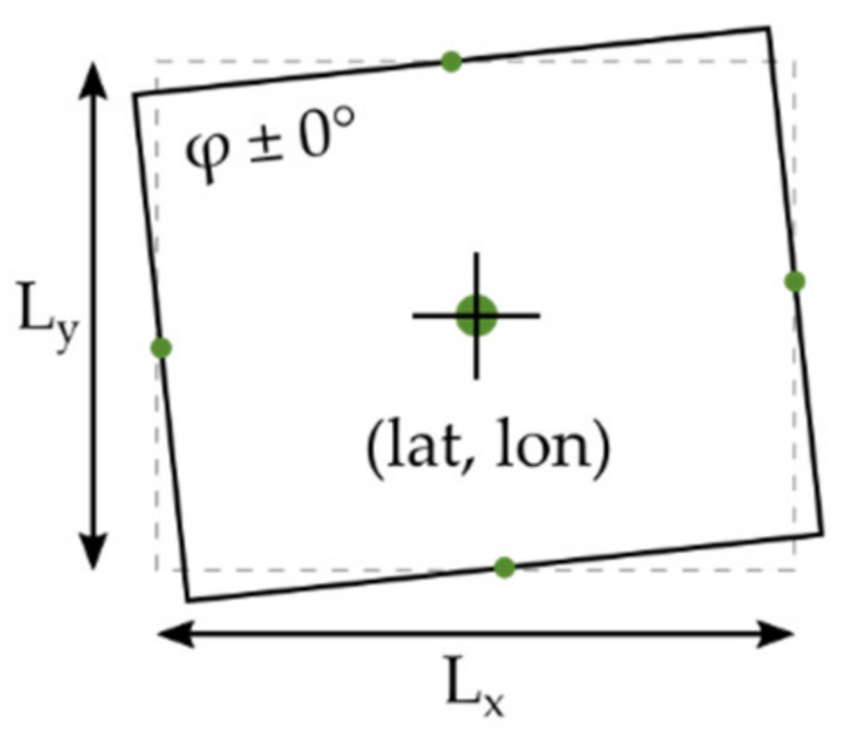
Before running the path profiling scrips, we define the footprint of the case building from the centre point in decimal degrees (lat, lon) by the length of the building envelope in the x-direction, length in the y-direction (in meter) and building rotation (in degrees). We specify the intermediate distance of mapping points for each façade and calculate their respective projection lines in all directions. Figure 2 shows the building and façade centre viewpoints used for the path profiling calculations (in green). In this way, it is irrelevant if the building is represented on the surface raster and building footprint shape layers or not.

2.1. Environmental Variables

2.1.1. Environmental Variables Derived from Reanalysis Data

Meteorological data (Table 1) were derived from the ERA5 atmospheric reanalysis of the global climate released by the European Centre for Medium-Range Weather Forecasts (ECMWF) as part of the Copernicus Climate Change Service (CDS). A comprehensive description of ERA5 is provided by Hersbach et al. [49]. ERA5 provides validated estimates for each hour of the day, worldwide, with a two to three months delay and leading back to 1979, or as recent as up to a couple of days ago through the preliminary dataset ERA5T.
Table 2 also shows selected variables from “ERA5-Land” another current dataset produced by ECMWF with around four times finer spatial resolution (~9 km grid spacing compared to the ~31 km grid of ERA5). It is a simulation of the land surface components of ERA5 forced by ERA5′s lower atmospheric fields, currently without coupling or additional data assimilation, meaning that observations only influence the simulation indirectly through the forcing [50].
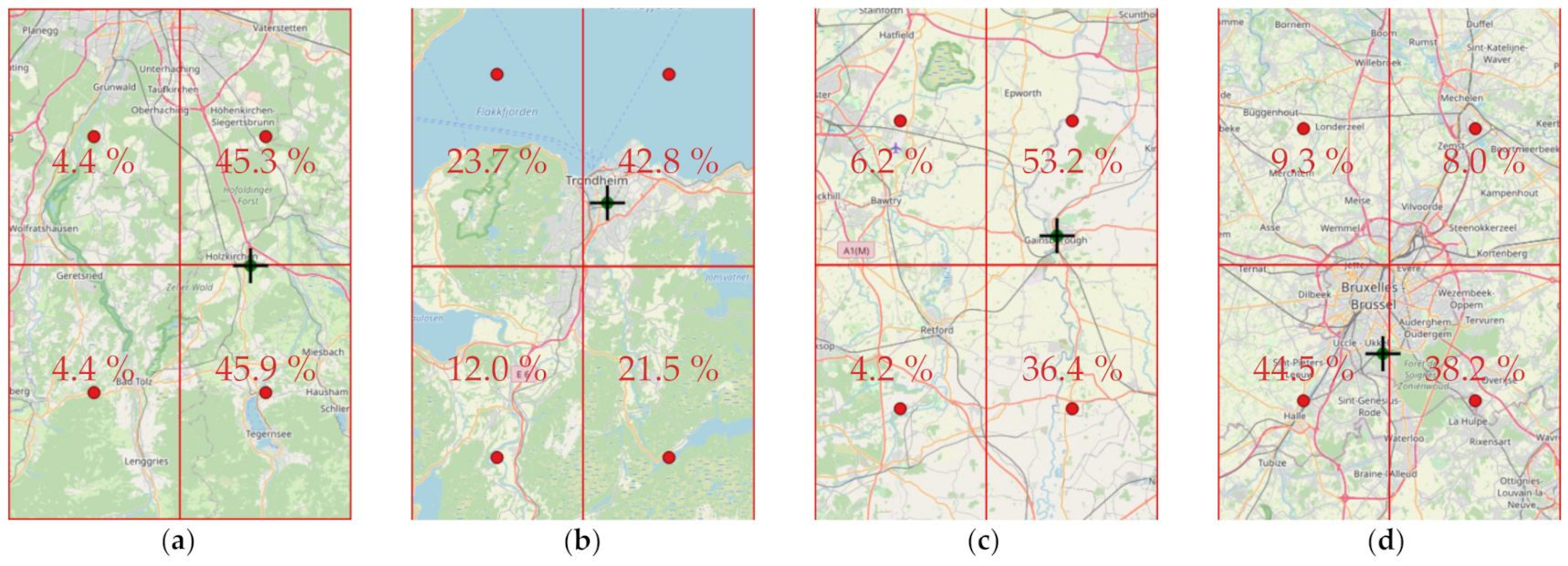
We used nearest-neighbour and bilinear interpolation to create hourly time-series for each site-location. Figure 3 shows the four case studies’ location relative to the ERA5 grid points and each grid tile’s relative weighting. The ERA5-land data were also interpolated to the site (not shown).

2.1.2. Environmental Variables Derived from Remote Sensing

For solar radiation, it is possible to use surface downwelling radiation from the reanalysis, but several studies show that better products exist to account for clouds’ variability. Services that combine solar models with remote sensing techniques provide greater temporal and spatial resolution. An overestimation of solar radiation is often observed in reanalysis, and an underestimation is observed in satellite methods [52].
Solar irradiance data were acquired from Copernicus Atmosphere Monitoring Service: CAMS Radiation Service (CAMS-Rad) version 3.2 [53]. CAMS-Rad’s satellite-based solar irradiance data are available at a spatial resolution of ~5 km over central Europe in 15-min time steps from 2004 until the present time (up to two days ago) and covers the field of view of the Meteosat satellite (Europe, Africa and the Middle East). An account of the radiative transfer scheme in CAMS-Rad is provided by Qu et al. [54]. We used the camsRad R-package [43] to obtain 1-min time-series of direct normal, global horizontal and diffuse horizontal irradiance for clear-sky and cloudy conditions. The dataset was then resampled to 10-min intervals for the shading calculations.

2.2. Downscaling

2.2.1. Local Wind Speed Estimation

The ERA5 reanalysis is already being applied in wind energy assessment, showing improvements over previously released global and regional reanalysis datasets [55,56,57]. In several recent studies, dynamical downscaling of ERA5 data using the high-resolution Weather Research and Forecasting (WRF) model has demonstrated an added value of introducing a higher spatial resolution [6,57,58]. The near-surface wind speeds in the reanalysis are advised not to be used directly to indicate surface wind conditions at a site [56], as the relatively low spatial resolution lacks the local representativity of the site surroundings. This recommendation is reflected by a word of caution in the API-documentation:
“Care should be taken when comparing this variable with observations because wind observations vary on small space and time scales and are affected by the local terrain, vegetation and buildings that are represented only on average in the ECMWF Integrated Forecasting System.”
In fact, the 10-m near-surface winds in ERA5 are parametrised as the potential wind in open terrain [59], which can differ substantially from the model representation over the whole grid cell [60]. Overland, exposure correction in ERA5 is done taking the lowest model level winds (at a height above the surface that is less influenced by underlining terrain) and applying vertical interpolation to 10 m through a logarithmic wind profile including stability indices (Monin-Obhukov theory). An open-terrain surface roughness (0.03 m) is used in the transformation [60].
In an attempt to better represent surface conditions, a simple analytical downscaling method is used. First presented by Wieringa [59], the “2L-method” consists of a two-layer model of the atmospheric boundary level to account for the difference in surface roughness from one location to another. It is to be used in combination with roughness lengths obtained through anemometric analysis or a surface roughness map. We used parts of the code as printed in [47] and a surface roughness conversion table (see Appendix C) for our implementation. Other more sophisticated models reported in the literature are included in the widely used commercial software WAsP, WindSim, and windPRO. There are similarities between the procedures implemented in WAsP, the 2L-method, and another simple model by De Rooy and Kok [61,62,63]. The latter was recently used to create a 1 km gridded dataset for Germany of hourly surface variables using station records and a regional climate reanalysis model [4]. Other authors have successfully combined WAsP and statistical approaches [6,64]. These simple downscaling methods are not claimed to represent the full complexity of the boundary layer. The 2L-method has mainly been used to create wind resource maps and determining extreme open-water winds [47,48,62,65]. It was first developed as an interpolation method for surface wind measurements [59] and has later been developed by Verkaik [66,67] and by Wever and Growen [68]. Evaluations over land have revealed mixed results, outlining that the roughness lengths significantly impact model performance and that the use of uniform (non-directional) roughness values leads to large errors [47,65,66,67].
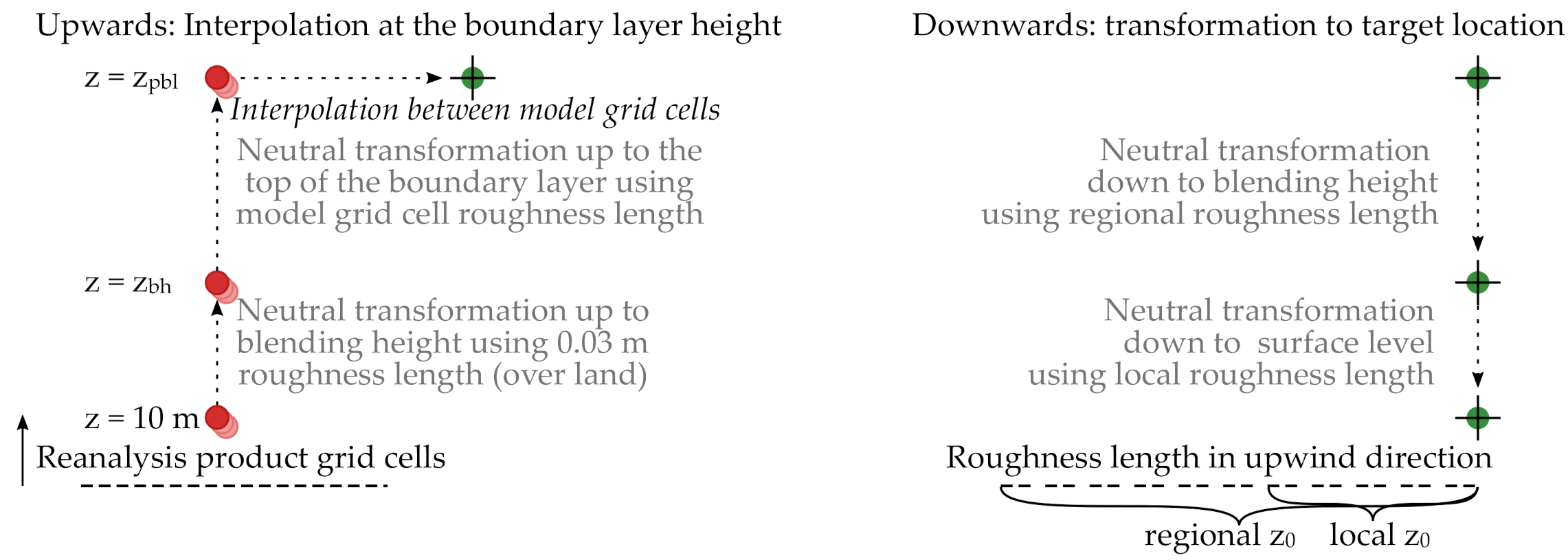
We follow the approach of Verkaik [66,67] using a high-resolution land-use map with derived surface roughness values together with a simplified footprint model to downscale model wind. In the lower level, the surface wind is transformed into the so-called blending height, where local disturbances have been blended out (Figure 4). Next, the wind speed in the upper layer is determined by using the NWP-model grid cell roughness value and geostrophic resistance laws [59]. At the height of the boundary layer, the wind speed is interpolated between model grid points to site. The wind speed at the blending height is calculated using regional surface roughness length and transformed back to surface height (10-m) using local roughness length in the given wind direction.
If the surface roughness used in the upwards and downwards transformation in the upper layer are identical (the model grid cell roughness and the regional roughness is set to the same value), the 2-layer model reduces to a neutral logarithmic wind profile conversion via blending height [59]. In the result section, we refer to this common conversion as the 1L-method:
U l o c = U 10 m ln z bh z 0 ; WMO ln z loc z 0 ; loc ln 10 z 0 ; WMO ln z bh z 0 ; loc ,   z 0 ; WMO = 0.03   m
where z loc is the local height to use in the conversion (10 m or roof height), z bh is the blending height, U 10 m is the wind speed from reanalysis, z 0 ; loc is the local roughness length at the target location and z 0 ; WMO is the open-terrain surface roughness (Equation (1)).
For the land cover classification, we use the CORINE land use (CLC) map covering the entire Europe. The map was stored in the elevation path profile web-service. The returned land cover classes along paths (with an intermediate spacing of 100 m) were used to assign their relative roughness using tables from literature (see Appendix C). The details of the regional and local roughness length calculation and the footprint model is given in the Appendix C.

2.2.2. Transforming Solar Irradiance Data Using a Satellite DEM

In CAMS Radiation Service, the irradiance calculations are done under the assumption of a flat terrain within the satellite pixel, without considering the diffuse parts masked or reflected by surrounding slopes [53]. In this study, no attempts are made to calculate the diffuse part reflected by the surrounding slopes, but it could be possible to use the satellite-derived DEM to calculate reflections. For the direct irradiance, to account for shading from local hills or mountains, we combined the matrices with the terrain shading angle from the JRC’s PVGIS API, selecting the two’s maximum shading angle in each sector. The PVGIS horizon angles were interpolated to match sectors of 2.5°, from the native 7.5° sectors corresponding to half-hour intervals. A distance of 10 km was assumed. Except for the PVGIS horizon profile API, no existing services were found to consider local hill-shading effects. Still, many web-based height map services provide tools to create elevation profiles manually along user-defined paths. We also want to test to what extent services that calculate terrain shading angle from satellite-derived DEM’s can supplement or substitute higher-resolution DSM’s/DTM’s covering the nearby building vicinity.

2.3. Transformations to Local Building Boundary Conditions Using Detailed Surface Models

2.3.1. Wind Shadow Sheltering on Facades by Nearby Upwind Obstacles

The wind shadow model to calculate wind sheltering effects on building air-infiltration is implemented into a Python script in the following work. The main concept of this simple empirical model first presented in Walker, Wilson and Forests 1996 paper [17], is a wind shadow projected downstream by upwind obstacles to determine the effect of wake velocity on the building surfaces. It applies a Gaussian-shaped weighting reduction, projected and weighted on the facades, that extends beyond the width of the obstacle in the far wake region. In the following, we apply the calculated directional sheltering factor to scale the wind speed in the infiltration model as intended in the original paper, not trying to solve the full wind profile with urban canyon effects, localised flow accelerations, vertical spread and other effects, which would be possible with CFD-simulation or with the three-dimensional diagnostic urban wind models described in the Appendix B that share the empirical parameterisation for far wakes [69,70]. In complexity level, the analytical model implemented here is more similar to the extensive work focusing on deriving wind conditions in urban environments using morphometric approaches [71].
The method calculates an effective mean wind speed U λ based on the unobstructed wind speed U , multiplied by the shelter factor λ w which takes a value between 1 (no shelter) to 0 (complete shelter), or 1 to 0.3 in a physical setting where large buildings are immediately adjacent [16]:
U λ = U · λ w θ
where the shelter factor λ w θ is expressed as a function of wind direction angle θ .
The authors of the wind shadowing method make it clear that the coefficients to find λ w and U λ (Equation (2)), were not based on measured wake velocities, but on measured sheltered and unsheltered façade surface pressures. See Appendix B for further discussion.
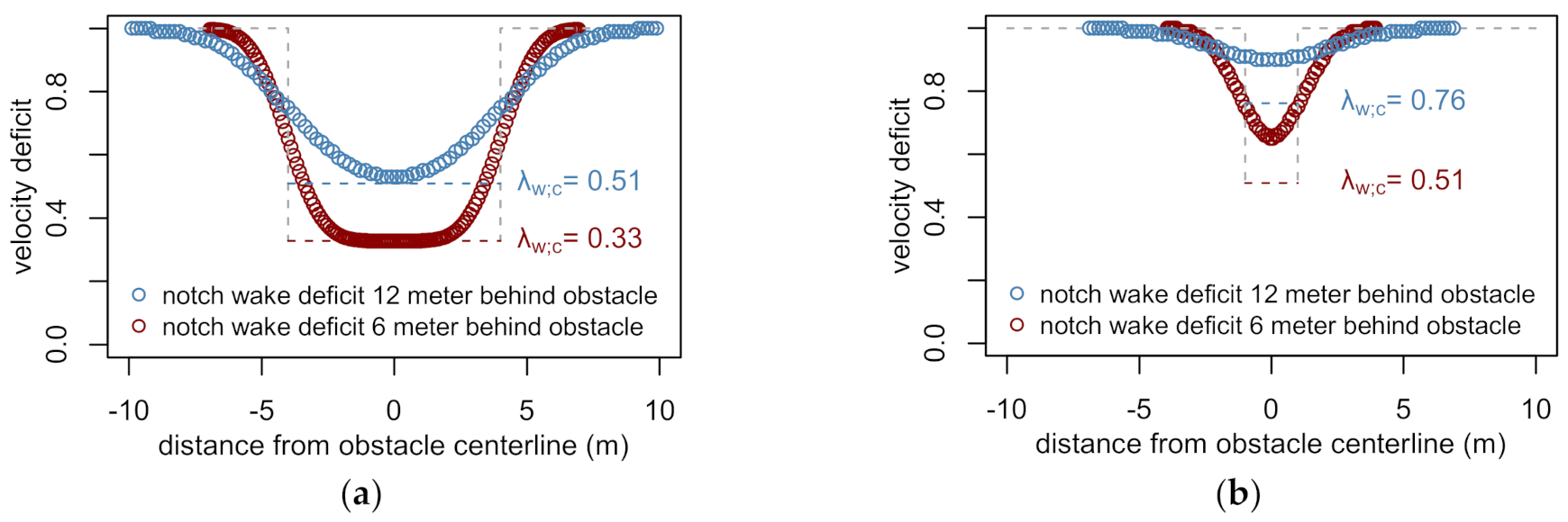
The other unique feature of the model is a flapped notch wake used to simulate the effect of wind direction fluctuations on near wake spread and growth. The notch wake indicated by notch centreline velocity in Figure 5, is flapped over a range of wind angles assuming a Gaussian distribution of wind direction about the mean angle θ :
λ w θ = j = 1 61 f ϕ j , θ , σ θ · λ w ϕ j
where the standard deviation of the wind distribution σ θ is estimated based on a function that changes with averaging time, e.g., 10° for a time-step of 1 h [17], which translates into a range ϕ j of +/− 30° for each side of the mean wind angle θ (Equation (3)).
Figure 5 illustrates how narrow and wide objects differ in notch wake velocity deficit and how fast the wake assumes a Gaussian profile behind the obstacle. A standard deviation of σ θ = 10° was used for the calculations (Equation (3)).
As described in Appendix B, to determine the scaling length, the obstacles’ aspect ratio is considered (calculating a characteristic dimension in the wind direction), but not including the roof pitch or edges of the obstacle relative to the wind direction, or the geometrical relationship between the two objects in consideration. These and other simplifications of the three-dimensional flows are discussed in the paper [17] and wind-tunnel experiments that evaluate the model [72]. Other studies show that although the assumption of wake symmetry may be a reasonable approximation for simple cubes oriented normal to the wind, for more complex geometries the functional form of the velocity deficit in the far wake is neither symmetric nor Gaussian [73,74]. For situations where the obstacle has protruding edges in the wind direction, standing vortices are formed that may lead to velocity deficits that differ significantly from what is predicted by a simple wake model [74].
In our implementation, the effective distance between the obstacle and the facade is calculated differently for the wind shadow coming into the facade, fully immersed, and out of the facade. When the projection line intersects with the façade, the distance is calculated from the intersection point to the obstacle’s edge. For the particular case, when the wind direction is perpendicular to the façade, the mid façade point is used in the distance calculation, which is the situation described in the paper.
For each façade, j, the effective shelter λ w ; j is found by a weighting of sheltered and unsheltered portions of the wall:
λ w = 1 1 λ w ; c L s L w
where λ w ; c ; j is the shelter factor on the wake centerline, L w ; j is the length of the façade, and L s ; j is the sheltered façade length (Equation (4)). The sheltered façade length and distance between the obstacle and the façade (the wake distance) will differ for each wall and wind angle. Every façade and obstacle are considered independently, and upwind walls do not shelter downwind building walls on the same building, as these effects are accounted for in the pressure coefficients [17].
The footprint of the building under consideration was defined as described in Figure 2. The nearby building footprints (including calculated mean building height information) were imported from building shape layers and analysed with Python’s shapely library. Trees and vegetation can be included as points (narrow obstacles), but this was not tested as there were no tall trees located within 2–3 building heights in the prevailing wind direction of either case building. Finally, we evaluate the maximum sheltering factor on each façade for every wind direction resulting in a combined directional sheltering factor for the building.

2.3.2. Approach to Calculate Sheltering from Surface Digital Elevation Models (DEM)

For the shading study, we created path profiling scripts using the gdal library for Python and later found Python modules of [45] and shifted to use these modules together with the elevation API. Calling the API repeatedly, one can use a façade sub-division, yet we restricted the evaluation to a single point per façade. For each case building, the digital elevation maps hosted in the elevation API covered a radius of at least 100 m around the building. Focusing on obstacles in the close surroundings is in agreement with Lingfors [31] who found that for roof surfaces a radius of 50 m is satisfactory with little impact on annual direct irradiance beyond 75 m. Further procedure:
(1)
Surface height and distance were evaluated extending at least e = 100 m outwards in each façade direction, using a spacing n of 1 m and a sector angle s of 2.5 degrees, creating matrices of dimension (e/n)   ·   (360/s), see also Figure 2 for illustration.
(2)
In the next step, the terrain reference height (above mean sea level) for the building and the façade height was used to calculate each sector’s maximum obstacle angle. We return the height and distance to this obstacle along with the obstacle height angle based on projection lines from mid-façade height, creating three arrays of (360/s) values for each façade. Knowing the façade orientations, the length of these arrays can optionally be reduced by half (to 180/s sectors).
(3)
To account for shading from local hills or mountains, we combined the matrices with the terrain shading angle from the EU-DEM mapping (up to 10 km) and the PVGIS API, selecting the maximum shading angle in each sector. The PVGIS horizon angles were interpolated to match sectors of 2.5°, from the native 7.5° sectors corresponding to half-hour intervals. A distance of 10 km was assumed to calculate PVGIS terrain height.
(4)
A fixed sky view factor was calculated for each façade orientation based on the mid-façade height horizon angle. Finally, the variable percentage of façade surface shaded by obstacles was calculated based on the full façade height, solar height and solar azimuth position according to the ISO52010 methodology. The selected 2.5° sectors correspond to 10 min intervals, making it straight forward to apply to 10-min time-series.
We start evaluating the horizon angle a few meters away from the façade to avoid heightmap slope artefacts or exclude trees or other nearby obstructions that are not shielding the entire façade. For the lower resolution DEMs, starting the evaluation, e.g., 5 m away also help to reduce how precisely the façade lines need to be defined relative to the underlying surface DEMs. Following the methodology laid out in the EN ISO 52016-1:2017 standard, it is suggested that building self-shading or “side-fins” are assessed separately.

2.3.3. Solar Shading by Nearby Objects

We follow the procedure of EN ISO 52016-1:2017 for calculation of solar shading reduction factors of nearby (and distant) objects. The standard differentiates between shading reduction factor by objects and on or close by the building itself like overhangs, sides and rebates. In the present work, we did not consider building self-shading. The standard gives two methods to assess shading of diffuse radiation; either disregard shading of the diffuse or use a sector-based evaluation applied to the Perez transposition model. In this anisotropic model, the diffuse part is separated into sky diffuse, circumsolar, horizon band and ground reflected irradiance (EN ISO 52010:2017 calculation method). The technical report accompanying the standard also outlines how some sky patch dome models are compatible with the Perez model. An example of implementing a sky patch model with Perez surface transposition and LiDAR data for shading analysis is found in [35]. As objects may not only block solar irradiance on a surface, but may also reflect solar radiation (e.g., hills, trees, other buildings, or other parts of the same building), the three-dimensional problem quickly calls for more advanced methods, e.g., ray-tracing supported by GPU acceleration. For simplicity, we follow the first approach in the standard, which is equivalent to a situation where the radiation reflected or transmitted by objects in the environment is equal to the diffuse radiation blocked by these object.
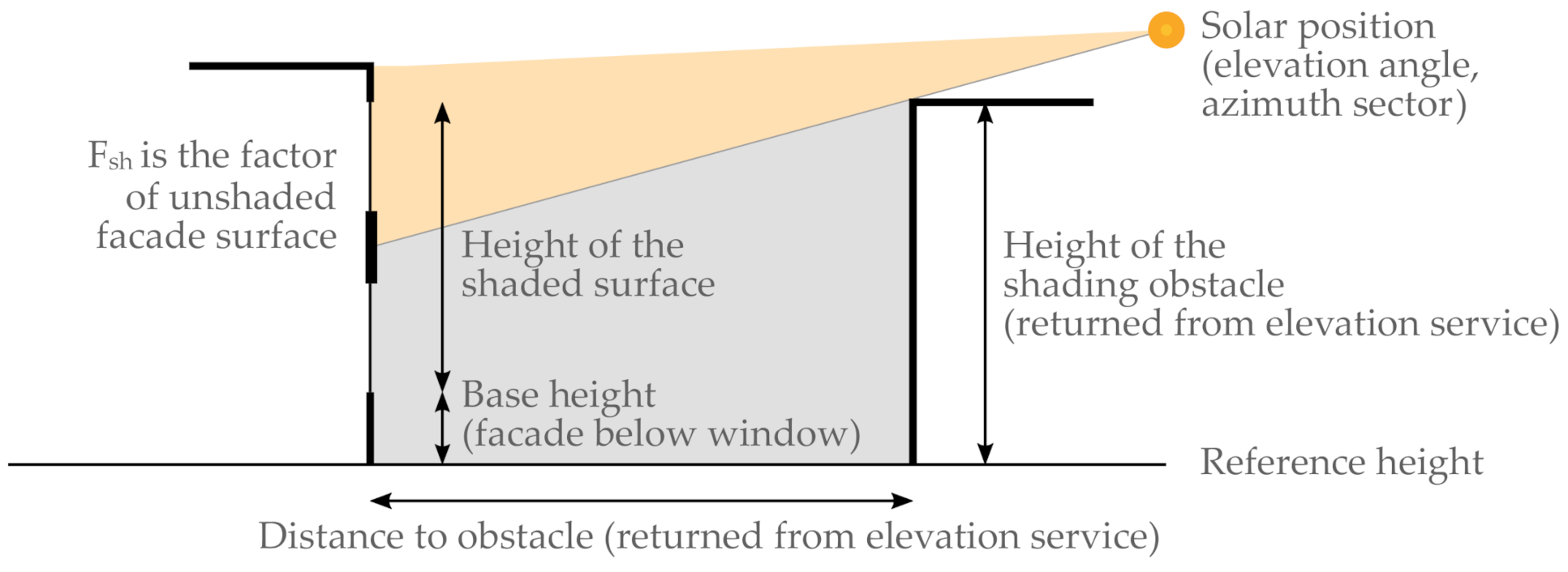
The direct radiation (including circumsolar) is fully or partially blocked by a factor Fsh if the object is between the sun and surface (Figure 6).

2.4. Including Environmental Variables and Local Sheltering Effects

In the following section, we discuss models that can be used pre-process weather variables in order to capture the thermal tie between indoor temperature, and boundary conditions, in this case, incident solar insolation and temperature- and wind-dependent air-leakages across the building envelope which result in infiltration losses.

2.4.1. Infiltration Losses

Infiltration is the uncontrolled air leakage through cracks and other unintentional openings in the building envelope introducing outdoor air into a building. Many infiltration models for residential buildings have been developed based on statistical fits of infiltration data. By considering that weather is the dominant driving force, infiltration flow can be assumed to be linearly dependent on the outside-inside temperature difference and wind-speed [75]. However, the simplicity of regression is not without limitations. The fitted coefficients carry little physical meaning, and the collinearity between heat transmission across the building envelope and infiltration losses driven by the indoor-outdoor temperature difference may lead to identifiability issues.
An empirical single-zone infiltration model accounts for infiltration, relying on physical parameters and building information, the AIM-2 model. We use the model form presented by Lundström in [58], where the calculated potential specific infiltration flow rate Qinf [Pan] multiples with the infiltration coefficient Cinf [l/(s Panm2)] which can be estimated by inverse approaches or obtained from fan pressurisations tests. A literature review of studies using the model and the differences in our implementation to [58] are presented in Appendix B. The single-zone infiltration models’ performance is mainly sensitive to the highly uncertain distribution of air leakages across the envelope and the parameters used for converting wind data measured at a weather station to the building site and local wind shelter effects from typography and nearby buildings. This uncertainty can be reduced by wind measurements on-site. However, shelter coefficient may still apply as a simplified approach to account for direct wind shielding caused by trees and neighbouring buildings located within 2–3 building heights of the building facades [16,17]. To estimate local wind velocity Uloc, AIM-2 uses unobstructed wind speed transformed to building eave height at the building site. A power law wind profile conversion was used in the original AIM-2 model, whereas a logarithmic wind profile conversion can be found in the implementation in the popular building energy simulation software ESP-r [76]. Furthermore, the wind shelter coefficient λw of 0–1 is multiplied by the wind speed at roof height. Both the authors of AIM-2 and the LBL infiltration method recommends making this shelter effect directional based on wind direction [16,75].
An engineering approach to make the wind sheltering directional is proposed by Walker and Wilson [16] and can be found reprinted in the ASHRAE Handbook of design guidelines [77]:
λ w θ = 0.5 · λ w ; 1 + λ w ; 3 · cos 2 θ + λ w ; 1 λ w ; 3 · cos θ +   λ w ; 2 + λ w ; 4 · sin 2 θ + λ w ; 2   λ w ; 4 · sin θ ,
where λ w θ   is the shelter factor for the particular wind direction θ , and   λ w ; j is the shelter factor when the wind direction is normal to a wall j (estimated perpendicular to each side building side) which can be estimated from sheltering class tables in literature [78].
We compare this interpolation approach (Equation (5)) to the wind sheltering model in the result section.

2.4.2. Solar Heat Irradiance on Facades

The solar irradiance is calculated as a weighted mean vertical input according to the proportions of total solar gains expected for each façade orientation. This input can be used in simplified thermal models that are suitable to determine building heat transmission losses (HTC) [79]. When measuring and accounting for solar gains in steady-state whole building heat loss experiments, one approach is weighting each façade by their respective glazing proportions. Stamp et al. found that for north-south oriented dwellings, vertical south-facing or weighted means provide the most accurate results to determine heat transmission losses (HTC), whilst estimating solar gains from global horizontal measurements overestimated HTC [80]. For east-west facing dwellings, mean or weighted means may provide more accurate results than a single vertical measurement in the dominant direction, particularly where there are local shading effects [80]. The presence and operation of solar shading devices represent a considerable uncertainty.

3. Results and Discussion

The proposed method is applied to four buildings:
  • The TWIN detached house oriented directly towards south at the Fraunhofer IBP test site in Holzkirchen, Germany.
  • The ZEBLL Living Lab detached house oriented south with 4° westward tilt on the main campus of NTNU, Trondheim, Norway.
  • The GBORO south-facing apartment end-unit oriented 12° eastwards in Gainsborough, UK.
  • The UKULE townhouse oriented 71° westwards from the south in a historic part of Brussels, Belgium.
Figure 7 illustrates that nearby buildings do not shade the east, south, and west façades of the TWIN house, at the 15. of February ca. 9:30 in the morning, 12:30 mid-day and 15.30-afternoon local time (or any other time in winter). The ZEBLL house at the NTNU campus, on the other hand, is shaded in the afternoon on this day from a nearby building located west of the house. We evaluate the shading model by using data from a pyranometer on the south façade in Section 3.2.

3.1. Comparison of Sourced Weather Data to Observations at the Holzkirchen Site

The key weather variables sourced from the reanalysis and the satellite irradiance service are presented, by comparing a two and a half month-long winter period to observations at the Fraunhofer IBP test site in Holzkirchen. The weather data was collected at the IBP’s weather station at 1-min intervals, provided as 10-min averages for the period 7 December 2018 to 28 February 2019 as part of IEA EBC Annex 71. The 10-min data were processed to hourly observations for the following analysis.

3.1.1. Air Temperature and Sky Longwave Irradiance

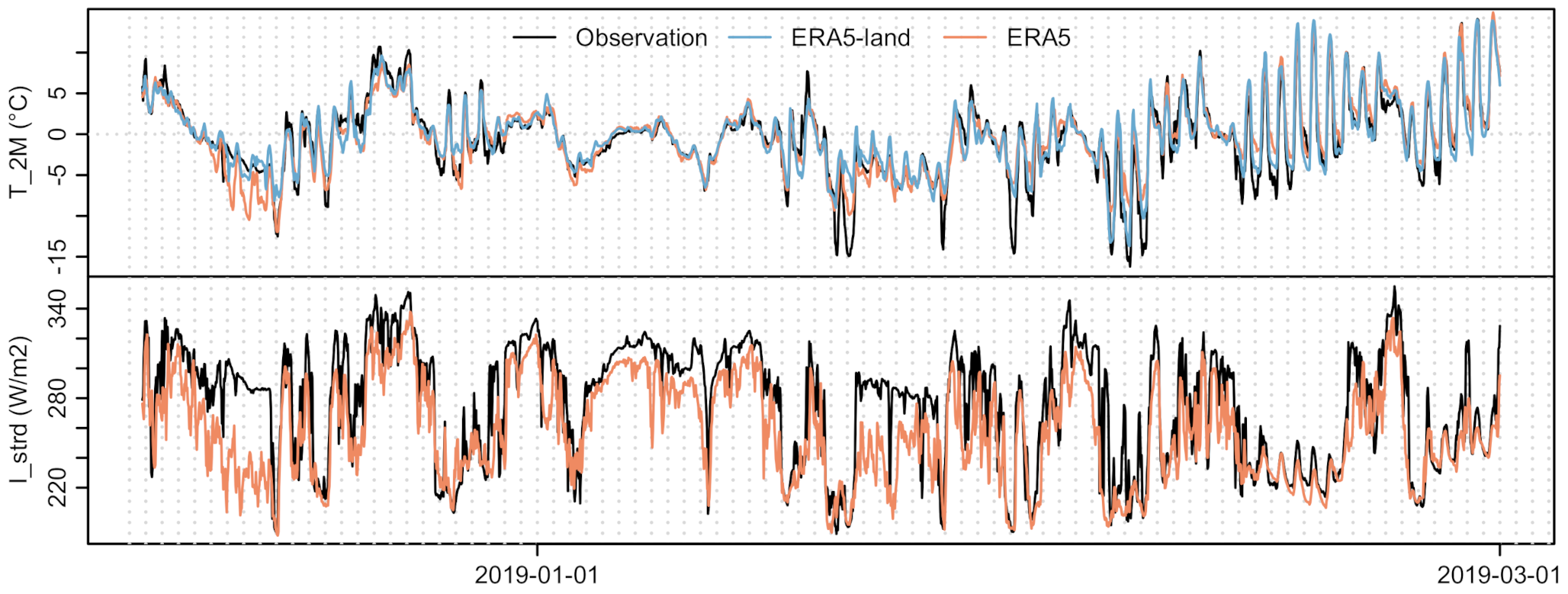
The air temperature and sky longwave irradiance from reanalysis are seen to represent the diurnal cycle (Figure 8). The ERA5-Land temperature at 2-m scores somewhat better on central performance metrics (0.33 °C, 2.04 °C and 1.36 °C) compared to ERA5′s (1.32 °C, 2.27 °C and 1.61 °C) for mean bias difference, root mean square error and mean absolute difference respectively. The errors are largest under cold spells. Both products underpredict the temperature under cold conditions, which is a feature of NWP models, they struggle to represent cold temperatures in stable conditions well [81].
The longwave sky irradiance and the sky temperature, calculated from the ERA5 longwave sky irradiance and air temperature (using the conversion in Table 2) correlate to local measurements on most of the days. In Figure 9, the distribution and sorted values in ascending order (black) reveal a bias across the distribution. These quantile-quantile plots are helpful to determine if the distributions are similar. The actual hourly values aligned in time are shown as coloured point samples. The reanalysis does not match observed hourly temperature in the lower end, but the distributions are similar, so more confidence can be placed for longer periods (e.g., monthly averages).

3.1.2. Wind Speed and Direction

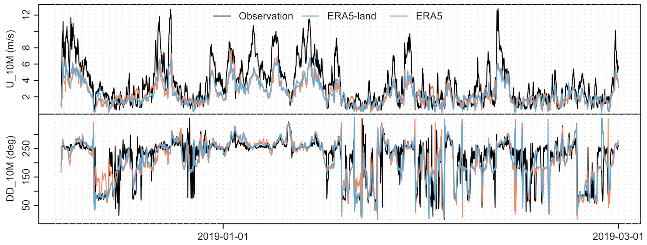
As described in the method section, the near-surface 10-m wind in the reanalysis is not itself a direct output of the model: instead, the lowest predicted model level wind is post-processed using an exposure correction to better represent observed 10-m wind in open terrain [60]. In this case, the wind mast’s local surroundings match the condition of open unobstructed terrain in the prevailing wind direction, making a direct comparison possible. When comparing the reanalysis data to site-observations, there is a clear bias in the reanalysis (Figure 10). Both products generally capture the hourly fluctuations reasonably but a consistent underprediction effect is observed.
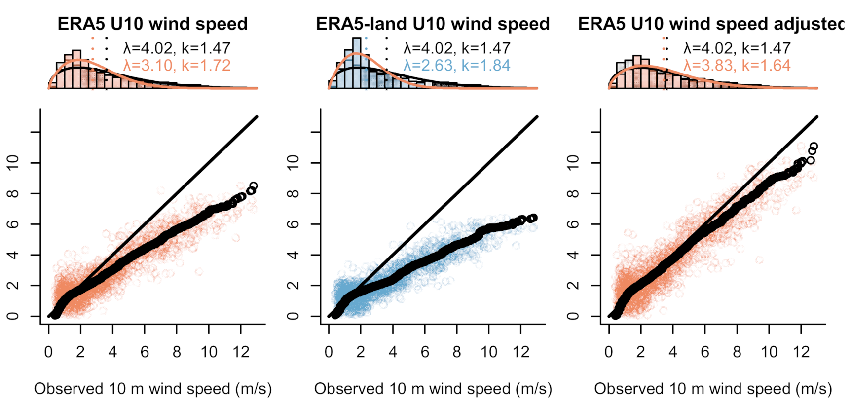
By applying the 2L-method, the 10 m near-surface wind from ERA5 is bias-adjusted, leading to a better match with the observed wind (Figure 11). More details on the correction factors are presented in the downscaling chapter. As with the temperature comparison, the actual hourly values aligned in time are shown as coloured point samples and sorted in ascending order (black) to see model bias across the theoretical distribution (Q-Q plot). A Weibull distribution is overlaid on top of each scatter plot, displaying the observations series in grey and the reanalysis in colours.
After the bias correction, the Weibull scale parameter is increased from 3.1 m/s to 3.8 m/s, compared to the observed 4.0 m/s. The mean bias difference is reduced from −0.85 m/s to −0.2 m/s, and the mean absolute difference is improved by 0.4 m/s from 1.2 to 0.8 m/s.

3.1.3. Global Horizontal and Diffuse Irradiance

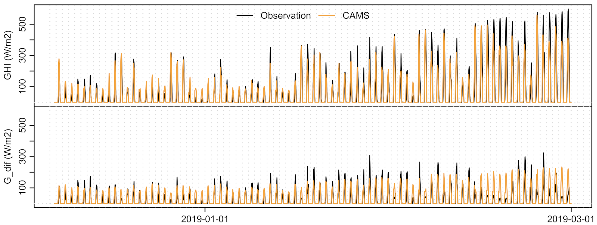
The global horizontal and diffuse irradiance observed at the site compares quite well to the satellite-derived irradiance from the CAMS-Rad service (Figure 12) on most days. There is a series of days in February, towards the end of the period, where diffuse irradiance is overpredicted, and the global horizontal is underpredicted. These are clear-sky days not interpreted as such by the satellite-model product. Earlier in the period, the cloud cover appears to be predominantly overcast (global horizontal and diffuse irradiance are equal), but some day-to-day variability can be spotted in both observations and satellite irradiances.

3.1.4. Snow Depth and Ground Surface Albedo

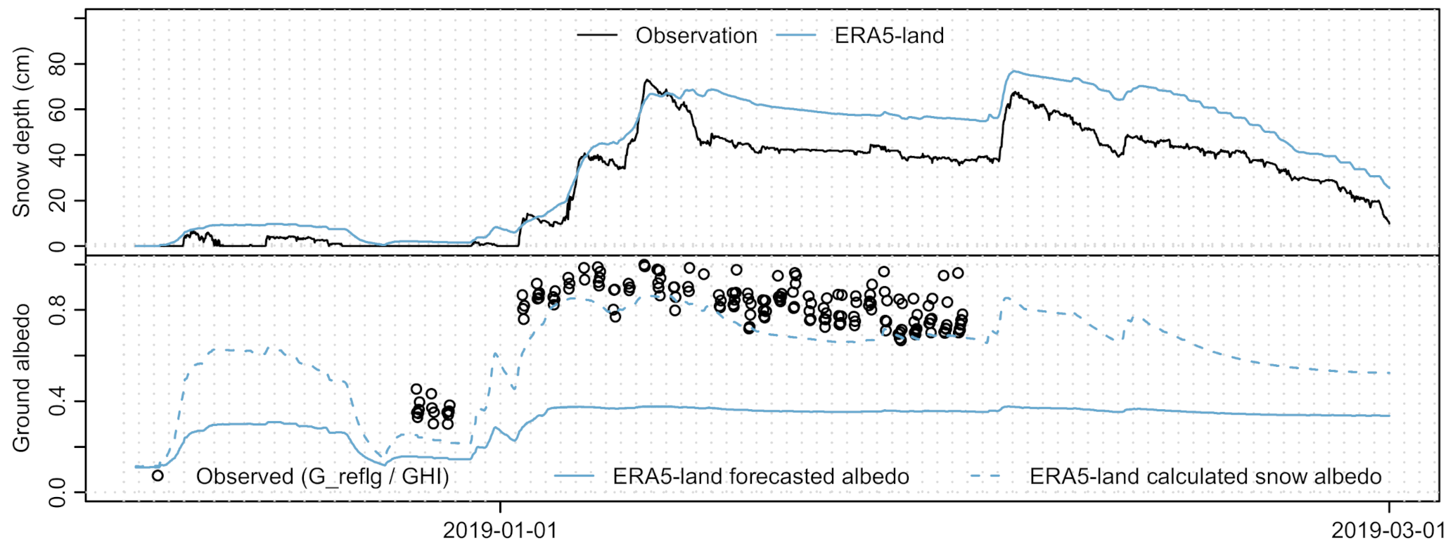
The snow model depth in the ERA5-Land grid cell matches the observed depth quite well (Figure 13). The calculated snow broadband albedo adjusted for snow cover (equation in Table 2) is compared to the measurements from two pyranometers on-site, filtered by solar azimuth height (only displaying values when the sun is 5° above the horizon) to account for uncertainty at sunrise and sunset. The uncertainty in the measurements is likely to be high at low radiation intensity, so applying more precise criteria could improve the correlation.

3.1.5. Vertical Solar Irradiance on Facades

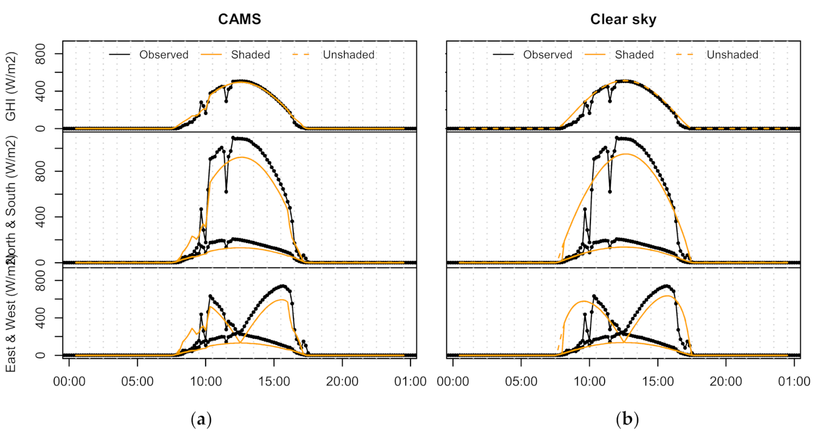
The TWIN buildings and weather station at the Holzkirchen site lie unobstructed in a flat open terrain making it impossible to evaluate the shading model with measurements from this site. It is still included to show the calculated horizontal and vertical solar irradiance compared to observations, as TWINS is the only case with measurements in all four façade orientations. On the particular day selected for analysis, clear sky conditions can be observed from ca. 10:00 in the morning (Figure 14). Even if the global horizontal irradiance from CAMS-Rad matches observations well, the calculated irradiance on each façade orientation is underestimated. We can observe that the diffuse fraction on the vertical appears to be underestimated in every facade direction even when using clear-sky irradiance as input to the solar transposition model. Possible explanations are due to how diffuse radiation is parametrised in the Perez anisotropic sky model (including model attenuation coefficients), the assumption that diffuse sky irradiance is isotropic in the shading calculations (each surface sees 50% of the sky) and physical effects caused by terrestrial reflectance or measurement errors. Due to fresh snow, the modelled ground reflectance was set to a high value of 0.70 at this day (calculated from the ERA5-Land snow cover).

3.2. Comparison of Sourced Weather Data to Observations at the NTNU Campus

Vertical Solar Irradiance on Facades

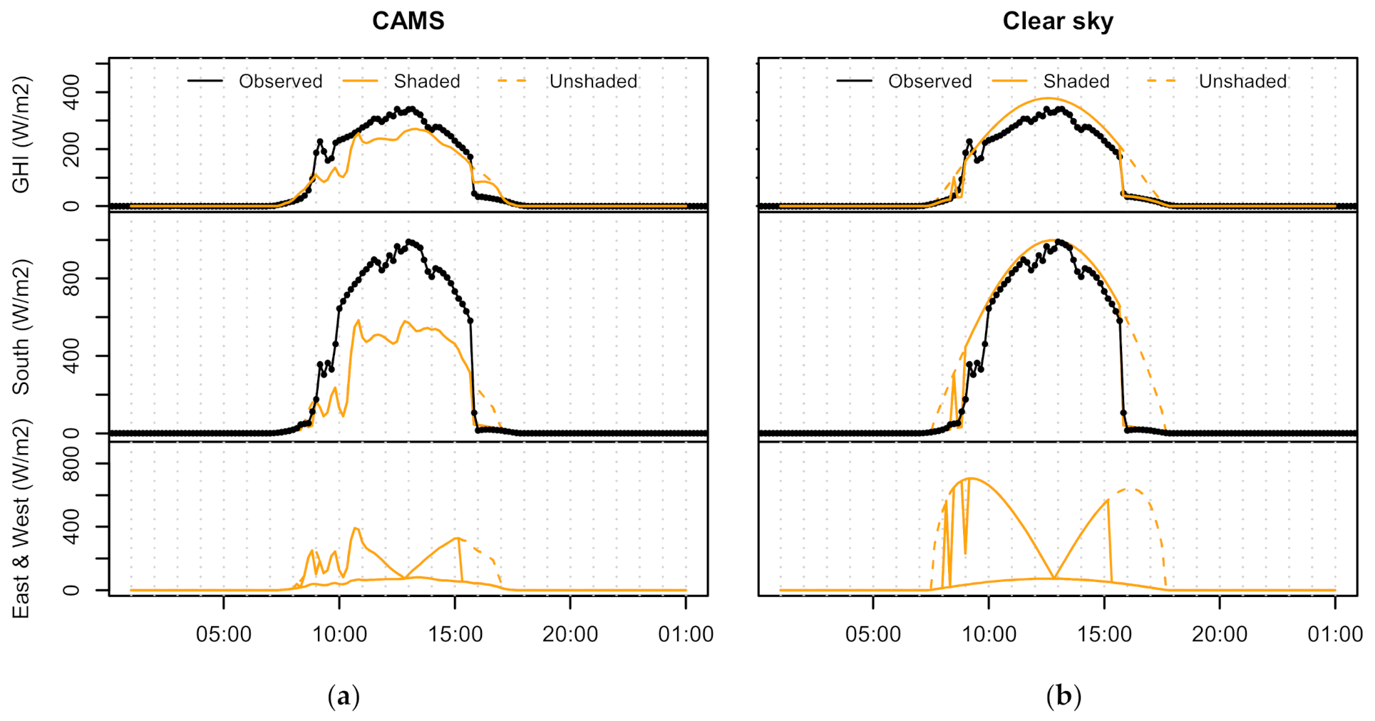
The ZEBLL campus building also features pyranometers measuring global horizontal irradiance on the roof and total vertical irradiance on the south façade. This building has its largest windows towards south, and the view from the wall-mounted sensor is shown in Figure 15. In winter, the afternoon sun is obstructed by large buildings towards west, well-captured by the shading model (Figure 16).
The CAMS-Rad irradiance over-evaluates cloud cover on this particular day (Figure 16a, but a better match can be seen in the clear sky irradiance from the CAMS-Rad McClear model (Figure 16b). The discrepancy on how vertical solar irradiance is calculated is likely due to surfaces partially shaded by trees before noon (Figure 15), because only buildings and terrain are considered in this particular diagram. The difference between observed hourly global horizontal irradiance and what is interpreted by the satellite product as mostly diffuse sky irradiance on this particular morning, also exemplifies how surface shading is left unaffected when cloud cover is predominant over the hour in the satellite product. Improving the shading calculations to include diffuse shading and not only effects on direct surface radiation.

3.3. Horizon Angle and Solar Radiation

3.3.1. Horizon Profile Using a Satellite-Derived Pan-European Surface Height Model

The proposed workflow for solar and wind assessment has in common that the same datasets are used on a local level, but in different ways. Moreover, that available dataset for downscaling to medium scale covers all of Europe (or global datasets), whereas the local effects are only assessable using local area height maps or building footprint vector map-layers with user contributed height-specification. Although there are initiatives of standardisation and contribution within the INSPIRE framework, including OSM contribution, and a community-led project to derive a pan-European terrain model online [82], high-resolution models involve more complex issues that are less pronounced in lower-resolution models due to the already high uncertainty. The EU-DEM v.1 product is evaluated to a vertical accuracy of 2.9 m RMSE, with higher values for the Nordic countries (e.g., 5.75 m RMSE for Norway) [83]. EU-DEM v1.1 used in this study is an improvement over the first version, but it has not been validated yet [23]. In order to use different datasets together, we implemented datum conversion and height adjustment to the different national height systems [82]. For Norway, the difference between the national height and the one used in EU-DEM was less than 1 cm, but for Belgium, the offset is as much as 2.31 m.
We tested combinations of height information from the EU-DEM model and the local high-resolution DSM’s. However, when mapping from the EU-DEM model surface height, which may very well be above the building height in steep terrain or in places with low buildings and heigh vegetation, we did not find a significant benefit to use the 30-m resolution of EU-DEM compared to the existing horizon profile API of PVGIS, which is a service that relies on a pre-processed global SRTM of 3 arc-seconds (around 90 m). However, we found that if we have actual information about the building elevation height, and create a buffer around the viewpoint (e.g., 50 to 100 m), we can create a horizon profile that in some situations is roughly similar to the detailed DSM’s.

3.3.2. Horizon Profile Using Local High-Resolution Surface Height Models

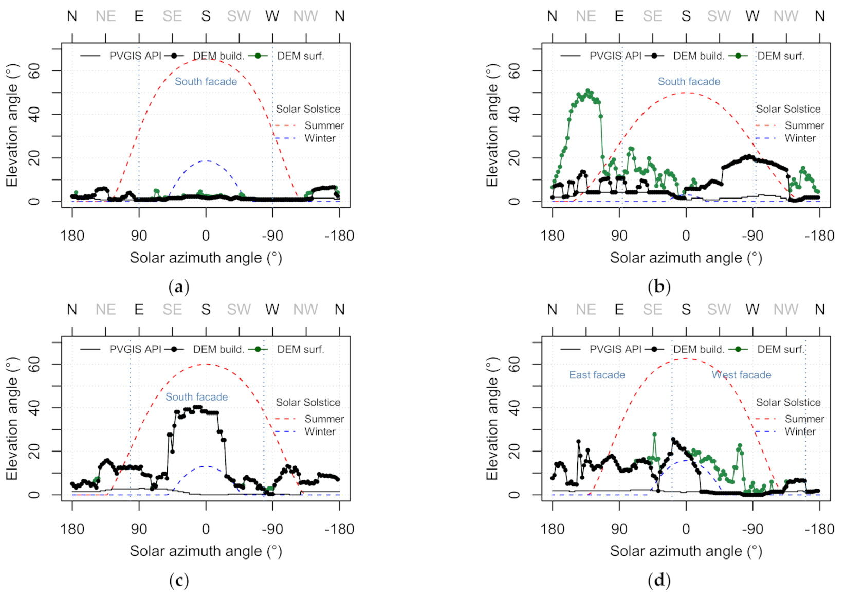
Figure 17, shows the calculated horizon angle at mid-façade height using the maximum local terrain profile of the PVGIS API (thin black line) and the high-resolution digital surface models filtered to buildings only (thick black line) or without filter (green), for the various case buildings. The TWINS building (a) is located in an open flat area. ZEBLL (b) is located in Norway where solar height at the summer solstice (red line) is lower than the others, and in this case, vegetation towards north-east and larger campus buildings westward block morning and afternoon sun. GBORO (c) is shaded by a neighbouring townhouse distanced 7 m from the south façade, and UKULE (d) is also located in an urban environment facing a street and a backyard with trees in the backyard.
Table 3 summarises the average calculated horizon height per façade, separated by considering only buildings obstacles (abbreviated “Build.”) or all obstacles including vegetation (abbreviated “Surf.”).
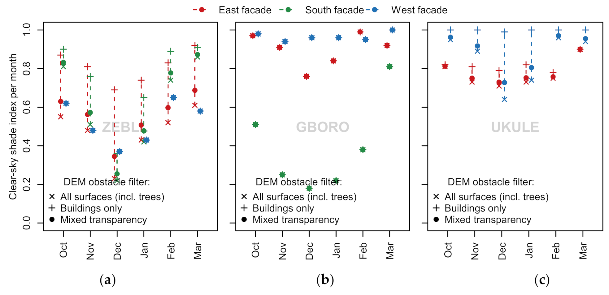
Figure 18 shows the clear-sky shade index per winter month by [31] defined as the ratio of shaded and unshaded clear-sky irradiance (only direct and circumsolar beam is included in the following). The impact of vegetation is presented as a range from fully opaque (by an x mark) to fully transparent (by a cross mark) and a mix of the two (dot).
-
For ZEBLL, the incoming direct radiation on the south and west façades is reduced substantially (up to 60%) by buildings in winter, and if trees are included, they may block beam insolation from south and east.
-
For the GBORO case building, trees have no shading impact, but the south façade is almost entirely in shadow from December to February, rapidly diminishing in March as the mid-day solar angle climbs.
-
For UKULE, which on average has moderate shading of vertical beam irradiance (ca. 20% reduction) on the two facades, the west façade is only shaded from vegetation.
By weighting the calculated surface radiation by the glazing ratios, we can estimate the solar heat gains on the window facades in the winter months and estimate a total solar aperture for the building.

3.4. Surface Roughness and Wind Sheltering

3.4.1. Unobstructed Height Adjusted Wind Speed

ERA5 has a model resolution of approximately 31 km and lack the local representativity of the site surroundings. To better represent surface conditions upwind influence, a downscaling method is used in an attempt to increase the local accuracy. The method consists of a high-resolution land-use map with derived surface roughness values from tables (Appendix A) and a simple two-layer model of the atmospheric boundary layer.
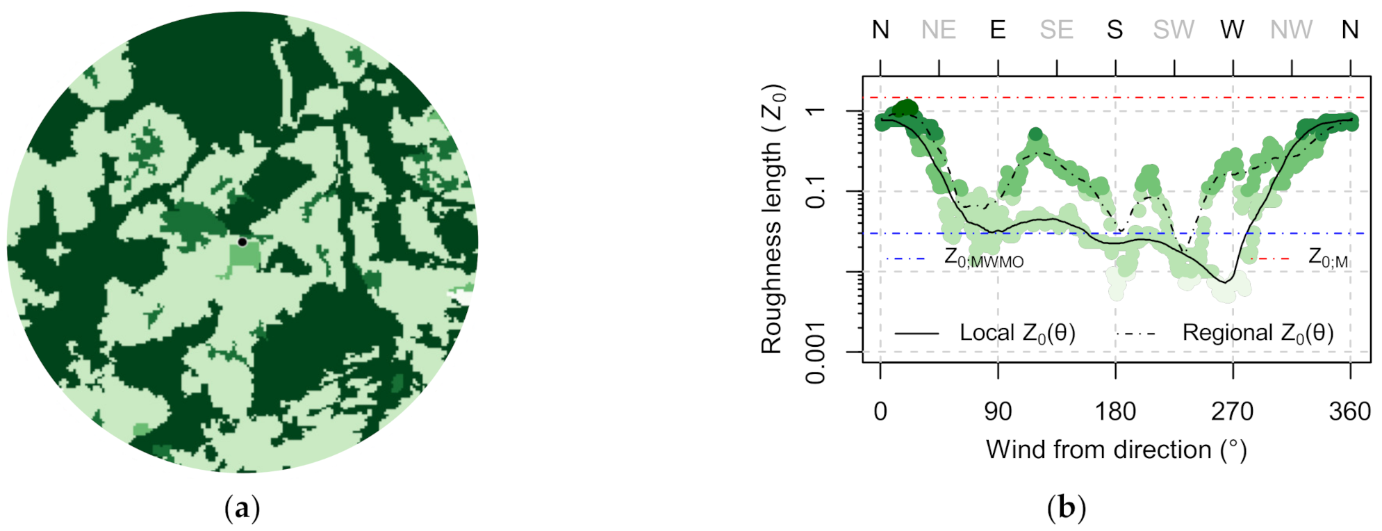
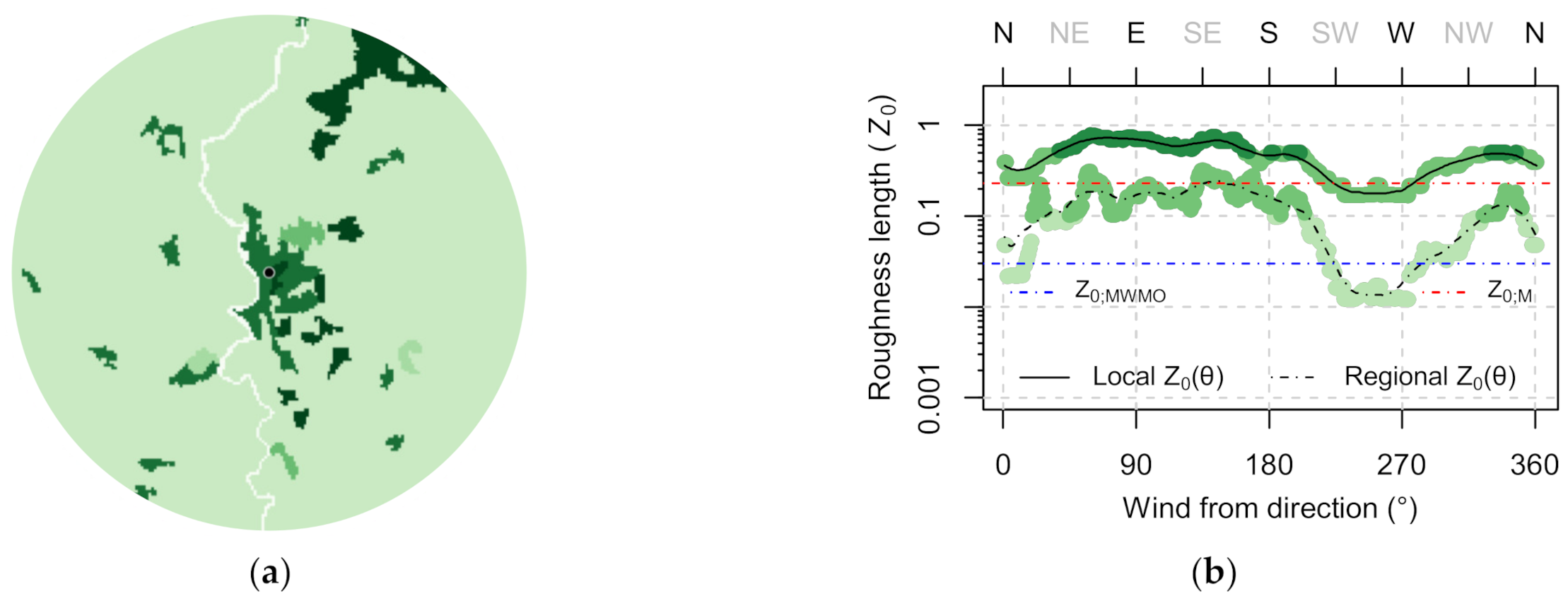
The analysis in Section 1 illustrated that 10-m surface wind speed at the Holzkirchen site (TWINS) is underestimated in the reanalysis. An explanation can be found in the high forecasted model surface roughness, indicating that the model grid box surface-average does not represent the local site conditions. The forecasted z 0 ; M   = 1.5 m (Table 4) is a value typically representative for forested areas. The site is located in an open agricultural area bordering the nearby town of Holzkirchen to the north-west and a golf course towards the south (Figure 9). The prevailing wind direction is west-south-west, and the first km up-wind are open landscape. Further out forest surrounds the farmland, influencing the regional scale weighted mean surface roughness plotted in Figure 17.
First, the forecasted surface roughness for each grid cell was extracted from the ERA5 reanalysis. Table 4 show the values for each site, together with the open terrain roughness used to compute 10-m wind in ERA and the derived surface roughness from the closest grid cell of the CORINE Land Cover (CLC) 2018 map paired with a table of roughness values (Appendix C). The roughness length for the land use type “Sport and leisure facilities” was adjusted to a lower value from 0.5 m to 0.03 m to represent the snow-covered golf course.
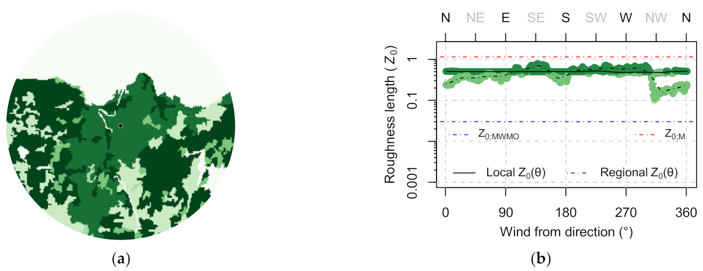
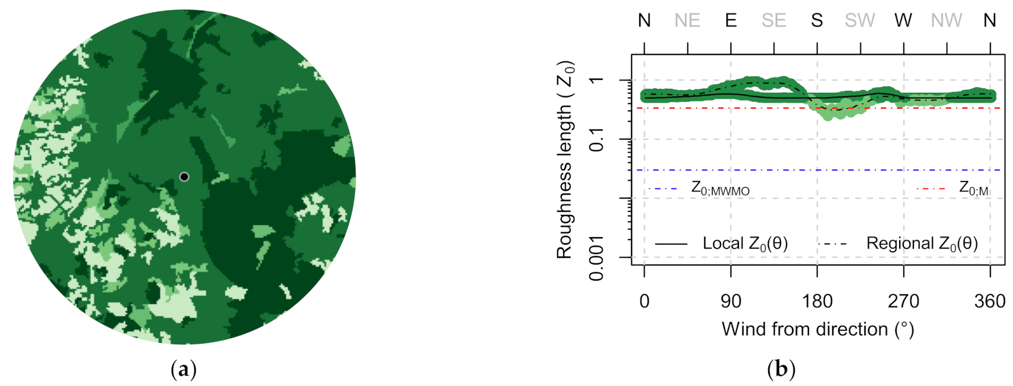
Next, the directional surface roughness from the footprint model applied to local scale (up to 1.8 km), and regional scale (up to 9 km) scale are plotted (Figure 19, Figure 20, Figure 21 and Figure 22). For TWINS we can see that on the local level, the surface roughness is well approximated to 0.03 m in the prevailing wind direction (SW), but the model level of 1.5 is many classes higher than the regional level z 0 , except in the north direction (due to the proximity to forest). The difference between the model average forecasted in the nearest grid cell ( z 0 ; M ), and the regional footprint model is less pronounced for cases (b) to (d) (Figure 20, Figure 21 and Figure 22). However, all display a considerably higher surface roughness on local-level than the open terrain roughness ( z 0 ; WMO ).
The resulting unobstructed surface winds transformed to roof height are used together with the wind sheltering method in the estimation of infiltration loss (see Section 3.4.3).

3.4.2. Wind Sheltering of Nearby Obstructions

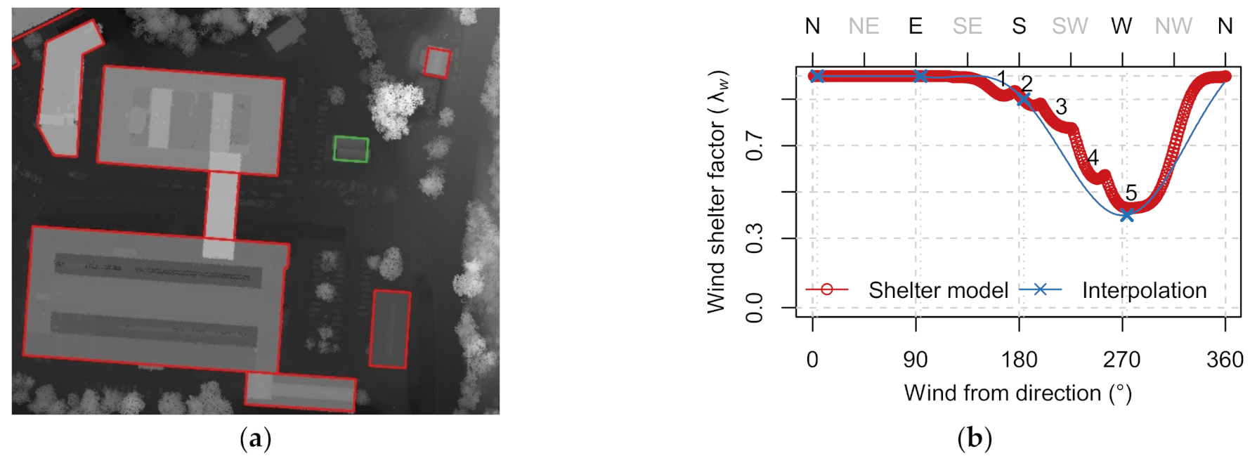
The wind sheltering model results are shown below for the three cases (b) to (d) where nearby buildings wake significantly impact surface conditions in the dominating wind direction. For the campus building (Figure 23), obstacles downwind coincide with the dominating south-west wind direction. Likely, these buildings will also influence the wind direction and lead to more complex airflow patterns than captured by the model.
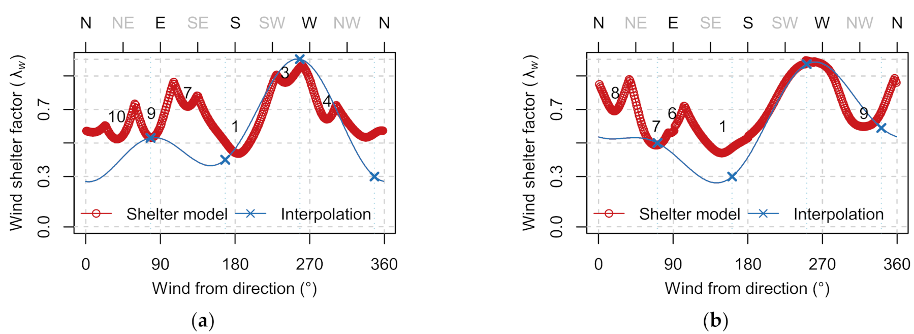
For the two other cases, GBORO and UKULE, located in urban/semi-urban setting, the calculated maximum sheltering coefficient from building obstacles are more irregular (Figure 24). Therefore, it fits less to the interpolated values (using Equation (5)) estimated qualitatively for each building side from sheltering classes in literature [78]. Instead of a selecting the sheltering factor manually from a table, one could use the model to approximate the sheltering factor from obstacles located perpendicular to each façade orientations (when the wind direction is normal to a wall).
In the presence of more tightly-spaced building obstacles, the limitations of the shelter-model implementation become evident. First, overlapping sheltering is not considered, which may be detrimental to performance. We have no way to assess skimming flow that is usually accounted for in urban wind morphometric approaches by increasing the zero-plane displacement height [71]. Secondly, with more complex and overlapping geometries, the functional form of the velocity deficit in the far wake is not Gaussian [72,73,74]. In the urban/semi-urban situation below, limiting the assessment to approximate the sheltering factor in the four façade directions and interpolating using Equation (5) may be a more physically sound and robust simplification.

3.4.3. Infiltration Loss

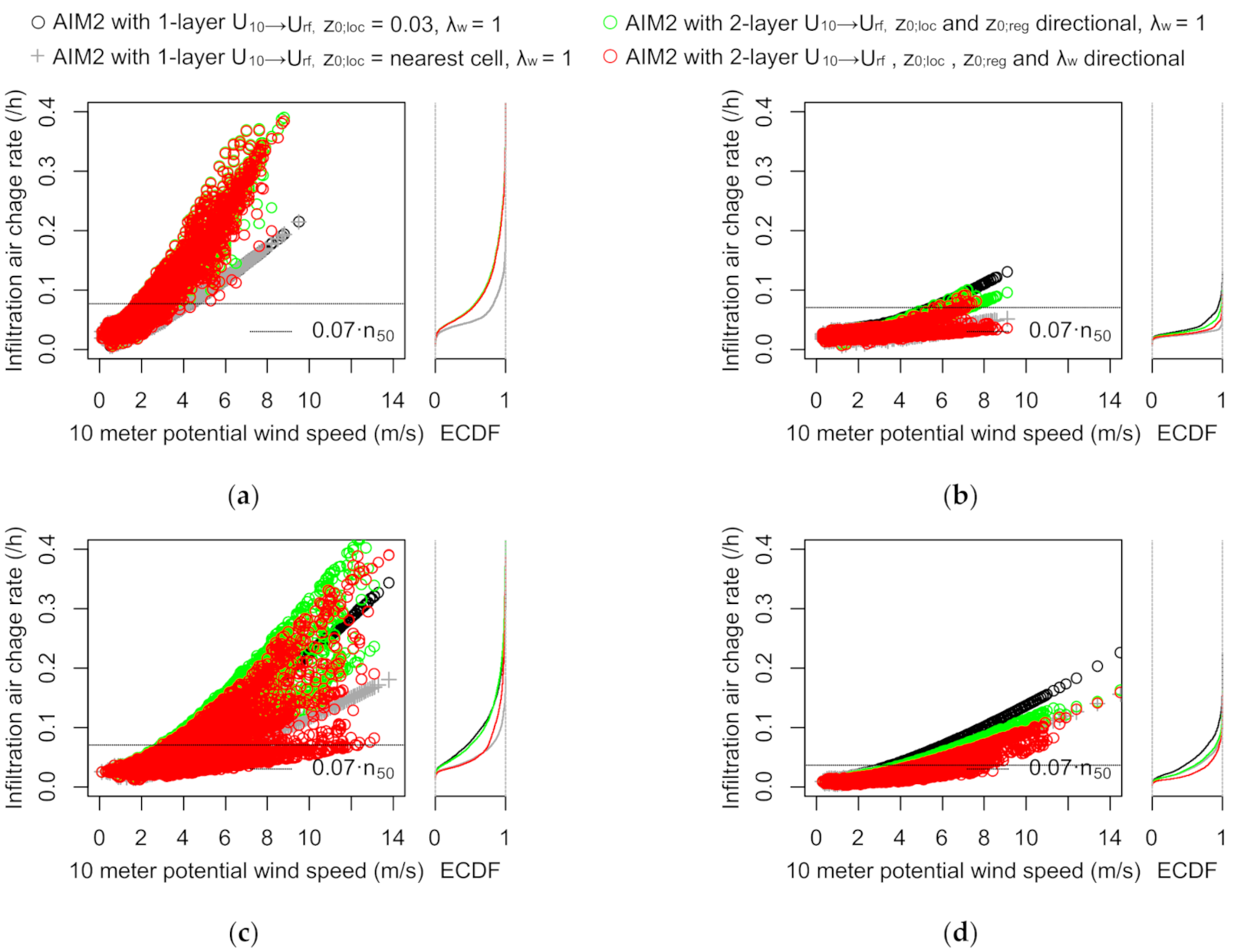
In this section, the infiltration model results are plotted against the potential wind speed of ERA5 at 10-m = height to illustrate the effect of the wind exposure and shelter correction. The AIM-2 models physical model output, “infiltration potential” (a scalable time-dependent variable) is multiplied by the results of air-pressurisation tests n50 value. It could be replaced by either a design-value or a parameter estimation in an inverse modelling approach. All the four cases (which are well-insulated and air-tight residential buildings) have measured air-pressurisation n50 values of 1.0 air change rate per hour at 50 Pa pressure difference, except the last case d) with a lower value of 0.5 h−1.
The slope of the infiltration air change rate at 1 atm. pressure (Figure 25) is mainly influenced by the n50 value, the shelter coefficient used in AIM-2 and what kind of exposure correction is made from ERA5 10 m potential wind speed (in open terrain) to building roof height, Urf.
  • The black horizontal line is a common conversion of the n50 infiltration rate to 1 atm. pressure, simply multiplying the n50 values by a constant of 0.07, a rule-of-thumb conversion factor representative of a moderately sheltered building with more than one exposed façade.
The first two AIM-2 model variants uses a 1-layer (1L) logarithmic transformation of the wind speed (up to a blending height of 60 m) which is a common conversion method in many Building Energy Simulation (BES) tools.
  • The black dots show the infiltration rate with a neutral logarithmic correction to roof height using the same surface roughness value of 0.03 m present in the reanalysis surface wind.
  • The grey crosses show the infiltration rate using a transformation from 10-m potential wind to roof height using a local roughness value. The local surface roughness obtained from the CLC-classification is 0.03 m for case (a) TWINS and 1.0 m for the other cases (Table 4).
In the last two AIM-2 model variants, the full 2-layer (2L) downscaling method was used with and without the directional surface sheltering method. In the 2L-method, the directional surface roughness upwind to the site is obtained for the required regional and local footprint using derived surface roughness from the CLC-classification.
  • The green points show the infiltration rate using the full 2L transformation of reanalysis wind.
  • The red points show the infiltration rate using the same 2L transformation with the directional surface sheltering method to account for nearby obstructions.
For the first two model runs using fixed surface roughness, the variability of air change comes from the outdoor indoor temperature difference, which is more pronounced at calm wind conditions. This effect is explained by the AIM2-models sub-addition of stack and wind-driven infiltration, where the stack effect loses significance at higher wind speeds. At higher wind speeds, the wind direction plays a role when the two-layer downscaling method is applied and through the wind shelter method in cases (b) to (d) where there are buildings located in the prevailing wind direction (Figure 25).
The resulting infiltration loss over the six-month winter period is presented in the table below in W/m2 K indoor-outdoor temperature difference and W/m2 assuming a constant indoor temperature of 21 °C in the period (Table 5). Consistent with the hourly infiltration air change rate (Figure 25), including shading from nearby obstacles significantly impacts the average infiltration heat loss over the winter period for cases (b) to (d). Comparing the average infiltration loss with nearby sheltering effect (final line) to the “rule-of-thumb” approach of scaling n50 by a constant of 0.07 (first line), the mean differences between the two are less than 30 % except for case b) ZEBLL.

4. Conclusions

In this paper we examine how open geospatial data can be used to refine weather variables for building energy performance evaluation with focus on incident solar radiation and wind-driven infiltration modelling. By using only building location (latitude, longitude) and a selection of free/open geospatial datasets covering Europe, we were able to acquire and adapt gridded weather data variables to local building boundary conditions. The nearly three-month-long winter comparison of a building test-site in South-Germany indicates that hourly surface variables from climate reanalysis and satellite-based solar radiation can become a feasible supplement to local observations for heating season building performance modelling and evaluation. However, the air temperature, vital to heating analysis, did not fully capture the extreme lows. In Europe, local observations of air-temperature and to some extent other weather variables are commonly available closer to site than the resolution of the current global reanalysis datasets (as was the case for the four case buildings). New regional surface products are expected to take advantage of observation stations’ density and reduce the need for site-correction techniques by featuring higher spatial resolution.
To include local effects from the terrain, vegetation and buildings in solar and wind assessments, 1-m resolution DSM’s and DTM’s from airborne laser scanning were acquired for each case building. The separation of nearby vegetation and buildings is essential to model incident solar insolation on low-rise building facades. The impact of distinguishing between the two was clear on the building-sites with trees. The separation was obtained by pre-processing the DSM into a new raster based on building outlines, but this operation could be made more efficient by using the Overpass API directly within the elevation profile web service to obtain building footprints and filter between building obstacles and vegetation. The building footprints (with building heights obtained from the DSM) were also used to include wind sheltering effects in the infiltration calculations. Including wind sheltering from nearby building obstacles in the AIM-2 model significantly impacts the average infiltration heat loss over the winter period for three of the four cases. Based on the four case studies, it seems like the approach work better for more open situations, other approaches may be better suited for buildings situated in a more dense urban setting.
Overall, we found that using scripting tools to automate geoprocessing tasks in conjunction with an elevation profile web service made it possible to utilise information from open geospatial data surrounding a building site effectively. However, there are needs for improvements to the methodology and risk of oversimplification. A next step could be to include diffuse-shading models and evaluate other wind conversions to site and shelter methods for urban settings. It appears that the often-scripted data-driven building thermal evaluation workflows can benefit from using climatological and spatial tools and datasets, especially to include local effects, but more practical evaluation studies are needed.

Author Contributions

Data curation, K.S.; Investigation, K.S.; Methodology, K.S.; Writing—original draft, K.S.; Writing—review and editing, K.S. and A.G.; Visualization, K.S.; Supervision, A.G. Both authors have read and agreed to the published version of the manuscript.

Funding

This paper has been written within the Research Centre on Zero Emission Neighbourhoods in Smart Cities (FME ZEN) funded by the Research Council of Norway (RCN), the research partners NTNU and SINTEF, and the user partners from the private and public sector.

Data Availability Statement

Produced using Copernicus data and information funded by the European Union-EU-DEM layers and Copernicus Land Monitoring Service, Copernicus Atmosphere Monitoring Service (CAMS) radiation service information and Copernicus Climate Change Service information–ERA5 and ERA5-Land global reanalysis. Contains DSM and DTM data produced by The Norwegian Mapping Authority/CC-BY 4.0, DSM and DTM data produced by the Environment Agency UK/Open Government Licence, DSM and DTM data produced by Information Flanders/Open Data Commons Attribution license 1.0, OpenStreetMap data © OpenStreetMap contributors/Open Data Commons Open Database License and Ordnance Survey data © Crown copyright and database right 2020.

Acknowledgments

The case studies were made available to participants in the IEA–EBC Annex 71 project Building Energy Performance Assessment Based on In-Situ Measurements.

Conflicts of Interest

The authors declare no conflict of interest.

Appendix A

Table A1. Building information and assumptions used to estimate solar irradiance on the facades. Façade glazing distribution and azimuth orientation are given in a list form where the four cardinal directions (N E S W) are (180 90 0 -90) degrees.
Parameter (N, E, S, W)TWINSZEBLLGBOROUKULE
Facade height hk4 m2.8 m5.0 m6.5 m
Aperture above gr. h0;k1.2 m0.6 m0.5 m1.7 m
Façade azimuth az (°)(180 90 0 -90)(176 86 -4 -94)(-168 112 12 -78)(-161 109 19 -71)
Glazing distribution fgl(.07 .21 .49 .23)(.19 .25 .40 .16)(0 .22 .39 .39)(0 .41 0 .59)
Window area Awi23.9 m239.3 m214.7 m240.1 m2
Frame factor Ffr;wi0.230.400.330.31
Transmittance ggl;n;wi0.670.50.670.67
Table A2. Building information and assumptions used in the building infiltration model.
ParameterCase 1Case 2Case 3Case 4
Floors Nfl21.524
Int. building height hb5.2 m3.4 m5.5 m11.3 m
Air tightness n501.0 h−11.0 h−11.0 h−10.5 h−1
Flow coefficient n0.670.670.670.67
Indoor temperature21212121

Appendix B

B.1. The AIM-2 Infiltration Model

A single zone infiltration model is used to account for building air-infiltration. Empirical single-zone infiltration models were developed in the 1980s and have seen some renewed interest in later years [84,85,86,87,88]. In most simplified infiltration models, the stack and wind-induced infiltration rates are assessed and derived separately and then superpositioned for a total infiltration rate. Two of the most established models are the LBL and AIM-2 models, adapted into simplified and advanced form in the ASHRAE Fundamentals Handbook. AIM-2 was developed by Walker and Wilson (1990) for houses [16], and a model implementation can be found in the BES software ESP-r [76].
The accuracy of the AIM-2 model to predict infiltration rates in dwellings can be excellent (±10%) when the model parameters are well known according to validations by the authors [78]. A separate validation study found a mean error of 16–27% assessing ten single-family homes [89]. Another study found an average error of about 19% predicting air infiltration rates for 16 detached houses under a wide range of weather conditions [84]. More recently, the AIM-2 model was utilised to predict infiltration rates in three stone-churches in Sweden [85]. The median absolute prediction error was 25%. Considering the model was not developed for large structures, a correction factor of 0.8 to account for overprediction was shown to reduce the error from 25 to 11%. In another recent study, the infiltration model was validated on a single building, obtaining a mean absolute value error of 17–35% by using different parameters for envelope leakage distribution [86]. A methodology is presented in successive work to determine the air change rate in near-real-time by combining the AIM-2 model with a tracer gas decay test method, reducing the error to 10% [90].
Lundström implemented the AIM-2 model in a building energy model [87], recently transformed to stochastic state-space form followed by a Bayesian calibration procedure [91]. The stochastic approach includes a logistic function to model occupant induced manual venting during heating and cooling season. Lundström presents the following version to calculate infiltration loss ϕ i n f in [87], where the calculated potential specific infiltration flow rate Qinf [Pan] multiples with the infiltration coefficient Cinf [l/(s Panm2)] which can be estimated or obtained from fan pressurisations tests.
ϕ i n f = C i n f · Q i n f · κ · ρ a · θ e θ i ,     Q i n f = Q / C i n f
Q i n f = Q s 1 n + Q w 1 n 0.33 · Q s · Q w 1 2 n n
where,   ρ a is the density of outdoor air, κ is the heat capacity, and exponent n is the building leakage flow coefficient of the orifice power law. Like many simple infiltration models, AIM-2 uses a superposition technique where the infiltration flow rates due to wind and stack effects, Q s and Q w , are added non-linearly in addition to an interaction term (Equations (A1) and (A2)).
In [87], building height H is adjusted for buildings taller than two floors to H* (m), resembling the correction factor used by [85] to account for over-prediction. Potential infiltration rates due to stack and wind effects can be pre-calculated by either using the calculated indoor temperature from the previous time-step in [91] or by assuming a constant pre-defined set-point temperature in [87].
Q s = f s Δ P s n = f s 9.806 · H · p a · θ e θ i θ i + 273.15 n
Q w = f w Δ P w n = f w 0.5 · U l o c 2 · λ w 2 · ρ a n
Assuming evenly distributed envelope leakage, no flue (chimney), and basement or slab-on-grade foundation, the wind and stack factors reduces to fs = 0.25 [(Pa/K)n] and fw = 0.22 [(Pa s2/m2)]. However, in this simplified form AIM-2 loses some of its flexibility to utilise building and site-specific data. The leakage distribution input values is a major source of uncertainty influencing AIM-2 and determining the values through measurements is difficult [78]. Noting a lack of reliable data, one of the validation studies shows that minor improvement is achievable (over the default uniform values) if certain building characteristics are taken into consideration [84]. Based on the optimisation of the leakage distribution (between ceilings, floors, and walls) on different groups of houses, their study recommends using values provided in a guideline for estimating leakage distribution parameters according to house types, number of storeys, and foundation type by Lew [92]. The leakage distribution tables by Lew were implemented as cited in the ESP-r source-code [76]. The full equations for fs and fw can be found in [78] including model forms for building flues or crawl spaces.

B.2. The Wind Shadow Method

The concept of a Gaussian-shaped wake in Walker, Wilson and Forest’s wind shadow method [17] is similar to a more commonly used shelter model “WEMOD” for far wake effects by Taylor and Salmon [65] that can be found implemented in the QUICK-URB and SkyHelios urban wind models [69,70]. Both QUICK-URB and SkyHelios are light-weight diagnostic urban wind models that do not solve the full Navier-Strokes equations but are based on empirical parameterisations, and mass conservation principles first compiled by Röckle [93] and later improved with updated parameterisations like the WEMOD wake model [69,70]. A difference between the wake model by Walker et al. and the WEMOD model is that the latter was developed to adjust wind speed measurements in a single point in space as opposed to being used on whole building facades. However, being of the same family of models many of the assumptions and limitations apply to both.
The sheltering factors were derived from measured sheltered and unsheltered surface pressures [17]. Therefore, the authors suggest that the surface pressure coefficients Cp of a building shielded by adjacent obstacles could be predicted by correcting the Cp obtained for an isolated building. This was later investigated in wind tunnel experiments using scale building models with different shapes and surrounding conditions by Sawachi et al. [72]. Their results indicate that the influence of the upwind building on the Cp distribution of the downwind building is clearly different inside and outside of the wind shadow. The best correlations are shown when the distance of an adjacent building (obstacle) is more than twice the obstacle’s height and width. It is suggested that when the adjacent building obstacle is closer, the width of the wind shadow should be given a wider area, depending on the depth of the shielding obstacle. Still, it is unclear from the paper whether they applied the flapping technique or simply projected a shadow of constant width. Another proposition is that the distance beyond where the shielding effect is negligible could be defined more clearly by the full three- dimensional size and geometrical relationship between the two objects in consideration [72].
For the scaling length in the model, a characteristic dimension of the obstacle is considered which is an empirical relationship between the smallest and the largest dimensions in projected width or height (cast in the direction of the wind). The definition is supported by former experimental studies. We refer to the original paper for the theoretical explanation of model assumptions and the functional form of the wake decay [17].

Appendix C

The roughness length table for each CLC type used in this work is published on the Finish wind atlas website with distinctive values for summer and winter. The values for winter are used.
To calculate the regional and local roughness length, a surface drag coefficient C d ; i is averaged at the blending height which is a method to give weighting to the larger roughness values [59,66]:
C d ; i = κ l n z b h / z 0 2   , κ = 0.4
where z b h is the blending height and z 0 is the roughness computed for each map point i (100 m). A simple footprint model is used to scale the significance of roughness further away from the site:
C d = W n C d ; i W n , W n = exp x n D
where the scaling factor D is 600 m for the local footprint and 3 km for regional footprint [66]. A source area of up to 3 times D is considered, resulting in an effective evaluation length of 1.8 km for the local scale and 9 km for the regional, which accounts for a total of 80% of the integral of Wn (Equation (A6)). Other studies using this footprint model have reported other distance weightings [48,63].

References

  1. Roth, M. The Use of Reanalysis in ASHRAE Applications. ASHRAE Trans. 2020, 126, 580–592. [Google Scholar]
  2. Qiu, X.; Roth, M.; Corbett-Hains, H.; Fuquan, Y. Mesoscale Climate Modeling Procedure Development and Performance Evaluation. ASHRAE Trans. 2016, 122, 186–201. [Google Scholar]
  3. Pelosi, A.; Terribile, F.; D’Urso, G.; Chirico, G.B. Comparison of ERA5-Land and UERRA MESCAN-SURFEX Reanalysis Data with Spatially Interpolated Weather Observations for the Regional Assessment of Reference Evapotranspiration. Water 2020, 12, 1669. [Google Scholar] [CrossRef]
  4. Krähenmann, S.; Walter, A.; Brienen, S.; Imbery, F.; Matzarakis, A. High-resolution grids of hourly meteorological variables for Germany. Theor. Appl. Climatol. 2018, 131, 899–926. [Google Scholar] [CrossRef] [Green Version]
  5. MET Norway NWP Wiki; GitHub: San Francisco, CA, USA. 2020. Available online: https://github.com/metno/NWPdocs/wiki/Post-processed-products (accessed on 12 October 2020).
  6. Dörenkämper, M.; Olsen, B.; Witha, B.; Hahmann, A.; Davis, N.; Barcons, J.; Ezber, Y.; García-Bustamante, E.; González Rouco, J.F.; Navarro, J.; et al. The Making of the New European Wind Atlas—Part. 2: Production and Evaluation. Geosci. Model Dev. 2020, 13, 5079–5102. [Google Scholar] [CrossRef]
  7. Udina, M.; Montornès, À.; Casso, P.; Kosović, B.; Bech, J. WRF-LES Simulation of the Boundary Layer Turbulent Processes during the BLLAST Campaign. Atmosphere 2020, 11, 1149. [Google Scholar] [CrossRef]
  8. Resch, B.; Sagl, G.; Törnros, T.; Bachmaier, A.; Eggers, J.-B.; Herkel, S.; Narmsara, S.; Gündra, H. GIS-Based Planning and Modeling for Renewable Energy: Challenges and Future Research Avenues. ISPRS Int. J. Geo Inf. 2014, 3, 662–692. [Google Scholar] [CrossRef]
  9. Biljecki, F.; Stoter, J.; Ledoux, H.; Zlatanova, S.; Çöltekin, A. Applications of 3D City Models: State of the Art Review. ISPRS Int. J. Geo Inf. 2015, 4, 2842–2889. [Google Scholar] [CrossRef] [Green Version]
  10. Lindberg, F.; Grimmond, C.S.B.; Gabey, A.; Huang, B.; Kent, C.W.; Sun, T.; Theeuwes, N.E.; Jrvi, L.; Ward, H.C.; Capel-Timms, I.; et al. Urban Multi-scale Environmental Predictor (UMEP). Environ. Model. Softw. 2018, 99, 70–87. [Google Scholar] [CrossRef]
  11. Altaweel, M. Python and Geospatial Analysis. Available online: https://www.gislounge.com/python-and-geospatial-analysis/ (accessed on 12 January 2021).
  12. ESRI ArcGIS REST API. Available online: https://developers.arcgis.com/rest/ (accessed on 10 December 2020).
  13. Biljecki, F.; Ledoux, H.; Stoter, J. Generating 3D city models without elevation data. Comput. Environ. Urban Syst. 2017, 64, 1–18. [Google Scholar] [CrossRef] [Green Version]
  14. Wendel, J.; Murshed, S.M.; Sriramulu, A.; Nichersu, A. Development of a Web-Browser Based Interface for 3D Data—A Case Study of a Plug-in Free Approach for Visualizing Energy Modelling Results. In Progress in Cartography; Springer: New York, NY, USA, 2016; pp. 185–205. [Google Scholar]
  15. European Commission. The INSPIRE Geoportal. Available online: https://inspire-geoportal.ec.europa.eu/ (accessed on 12 November 2020).
  16. Walker, I.S.; Wilson, D. The Alberta Air Infiltration Model: AIM-2; Department of Mechanical Engineering, University of Alberta: Edmonton, AL, Canada, 1990. [Google Scholar]
  17. Walker, I.S.; Wilson, D.J.; Forest, T.W. Wind Shadow Model for Air Infiltration Sheltering by Upwind Obstacles. HVAC&R Res. 1996, 2, 265–282. [Google Scholar]
  18. Coetzee, S.; Ivánová, I.; Mitasova, H.; Brovelli, M.A. Open Geospatial Software and Data: A Review of the Current State and A Perspective into the Future. ISPRS Int. J. Geo Inf. 2020, 9, 90. [Google Scholar] [CrossRef] [Green Version]
  19. Clarke, J.A. Why Tools for Buildings and Cities Performance Simulation Need to Evolve. Available online: https://www.buildingsandcities.org/insights/commentaries/tools-for-buildngs-and-cities-performance.html (accessed on 28 December 2020).
  20. Clarke, J. IOP Simulation-Based Procedure for the Holistic Resilience Testing of Building Performance. In Conference Series: Earth and Environmental Science; IOP Publishing: Bristol, UK, 2019; p. 12027. [Google Scholar]
  21. Manfren, M.; Nastasi, B.; Groppi, D.; Astiaso Garcia, D. Open data and energy analytics—An analysis of essential information for energy system planning, design and operation. Energy 2020, 213, 118803. [Google Scholar] [CrossRef]
  22. Copernicus Land Monitoring Service. CORINE Land Cover. 2018. Available online: https://land.copernicus.eu/pan-european/corine-land-cover/clc2018 (accessed on 15 May 2020).
  23. Copernicus Land Monitoring Service. EU-DEM v1.1. Available online: https://land.copernicus.eu/imagery-in-situ/eu-dem (accessed on 15 May 2020).
  24. Tabas, D.; Fang, J.; Porté-Agel, F. Wind Energy Prediction in Highly Complex Terrain by Computational Fluid Dynamics. Energies 2019, 12, 1311. [Google Scholar] [CrossRef] [Green Version]
  25. Silva, J.; Ribeiro, C.; Guedes, R.; Rua, M.-C.; Ulrich, F. Roughness length classification of Corine Land Cover classes. In Proceedings of the EWEC, Milano, Italy, 7–10 May 2007; Citseer: Princeton, NJ, USA, 2007. [Google Scholar]
  26. NASA Land Processes Distributed Active Archive Center (LP DAAC). Available online: https://lpdaac.usgs.gov/ (accessed on 12 November 2020).
  27. Szypuła, B. Quality assessment of DEM derived from topographic maps for geomorphometric purposes. Open Geosci. 2019, 11, 843–865. [Google Scholar] [CrossRef]
  28. Huld, T. PVMAPS: Software tools and data for the estimation of solar radiation and photovoltaic module performance over large geographical areas. Sol. Energy 2017, 142, 171–181. [Google Scholar] [CrossRef]
  29. Statens Kartverk Høydedata. Available online: https://hoydedata.no/ (accessed on 10 September 2020).
  30. Bayerische Vermessungsverwaltung. Gebühren- und Preisliste für Geobasisdaten der Bayerischen Vermessungsverwaltung. 2020. Available online: ldbv.bayern.de/file/pdf/1269/Preisliste_aktuell.pdf (accessed on 15 April 2020).
  31. Lingfors, D.; Bright, J.M.; Engerer, N.A.; Ahlberg, J.; Killinger, S.; Widén, J. Comparing the capability of low- and high-resolution LiDAR data with application to solar resource assessment, roof type classification and shading analysis. Appl. Energy 2017, 205, 1216–1230. [Google Scholar] [CrossRef]
  32. Buffat, R.; Grassi, S.; Raubal, M. A scalable method for estimating rooftop solar irradiation potential over large regions. Appl. Energy 2018, 216, 389–401. [Google Scholar] [CrossRef]
  33. Redweik, P.; Catita, C.; Brito, M. Solar Energy potential on roofs and facades in an urban landscape. Sol. Energy 2013, 97, 332–341. [Google Scholar] [CrossRef]
  34. Brito, M.C.; Redweik, P.; Catita, C.; Freitas, S.; Santos, M. 3D Solar Potential in the Urban Environment: A Case Study in Lisbon. Energies 2019, 12, 3457. [Google Scholar] [CrossRef] [Green Version]
  35. Lindberg, F.; Jonsson, P.; Honjo, T.; Wästberg, D. Sol. Energy on building envelopes—3D modelling in a 2D environment. Sol. Energy 2015, 115, 369–378. [Google Scholar] [CrossRef]
  36. Chen, Z.; Gao, B.; Devereux, B. State-of-the-Art: DTM Generation Using Airborne LIDAR Data. Sensors 2017, 17, 150. [Google Scholar] [CrossRef] [PubMed] [Green Version]
  37. Nex, F.; Remondino, F. UAV for 3D mapping applications: A review. Appl. Geomat. 2014, 6. [Google Scholar] [CrossRef]
  38. Puente, I.; Gonzalez, H.; Arias, P.; Armesto, J. Land-Based Mobile Laser Scanning Systems: A review. Int. Arch. Photogramm. Remote Sens. Spat. Inf. Sci. 2011, 38. [Google Scholar] [CrossRef] [Green Version]
  39. Brovelli, M.A.; Zamboni, G. A new method for the assessment of spatial accuracy and completeness of OpenStreetMap building footprints. ISPRS Int. J. Geo Inf. 2018, 7, 289. [Google Scholar] [CrossRef] [Green Version]
  40. Fan, H.; Zipf, A.; Fu, Q.; Neis, P. Quality assessment for building footprints data on OpenStreetMap. Int. J. Geo Inf. Sci. 2014, 28, 700–719. [Google Scholar] [CrossRef]
  41. Hjelseth, E.; Thiis, T. Use of BIM and GIS to enable climatic adaptations of buildings. In Ework and Ebusiness in Architecture, Engineering and Construction; Christodoulou, S., Scherer, R., Eds.; CRC Press Taylor & Francis Group: Boca Raton, FL, USA, 2008; pp. 409–417. [Google Scholar]
  42. Hufkens, K.; Reto, S.; Campitelli, E. ECMWFR: Programmatic Interface to the Two European Centre for Medium-Range Weather Forecasts API Services; Version 1.2.0; Zenodo: Meyrin, Switzerland, 2019. [Google Scholar]
  43. Lundström, L. CamSrad: Client for CAMS Radiation Service; Version 0.3. 0; R Package; R Core Team: Vienna, Austria, 2016. [Google Scholar]
  44. Nisbet, A. Open Topo Data; GitHub: San Francisco, CA, USA, 2020; Available online: https://github.com/ajnisbet/opentopodata/ (accessed on 11 November 2020).
  45. Peronato, G. getHorizon; Laboratory of Integrated Performance in Design (LIPID), Ecole Polytechnique Fédérale de Lausanne (EPFL): Lausanne, Switzerland, 2017. [Google Scholar]
  46. Lundström, L. Total Solar Irradiance According to ISO 52010-1:2017; GitHub: San Francisco, CA, USA, 2018; Available online: https://github.com/lukas-rokka/solarCalcISO52010 (accessed on 2 May 2020).
  47. Stepek, A.; Wijnant, I.L. Interpolating Wind Speed Normals from the Sparse Dutch Network to a High Resolution Grid Using Local Roughness from Land Use Maps; Royal Netherlands Meteorological Institute: De Bilt, The Netherlands, 2011. [Google Scholar]
  48. Caires, S.; de Waal, H.; Groeneweg, J.; Groen, G.; Wever, N.; Geerse, C.; Bottema, M. Assessing the uncertainties of using land-based wind observations for determining extreme open-water winds. J. Wind Eng. Ind. Aerodyn. 2012, 110, 70–85. [Google Scholar] [CrossRef]
  49. Hersbach, H.; Bell, B.; Berrisford, P.; Hirahara, S.; Horányi, A.; Muñoz-Sabater, J.; Nicolas, J.; Peubey, C.; Radu, R.; Schepers, D.; et al. The ERA5 global reanalysis. Q. J. R. Meteorol. Soc. 2020, 146. [Google Scholar] [CrossRef]
  50. Muñoz Sabater, J. First ERA5-Land dataset to be released this spring. ECMWF Newslett. 2019, 159, 8–9. [Google Scholar]
  51. Hogan, R. Radiation Quantities in the ECMWF Model and MARS. Technical Report ECMWF. 2015. Available online: https://www.ecmwf.int/node/18490 (accessed on 10 April 2020).
  52. Babar, B.; Graversen, R.; Boström, T. Solar radiation estimation at high latitudes: Assessment of the CMSAF databases, ASR and ERA5. Sol. Energy 2019, 182, 397–411. [Google Scholar] [CrossRef]
  53. Schroedter-Homscheidt, M.; Hoyer-Klick, C.; Killius, N.; Betcke, J.; Lefèvre, M.; Wald, L.; Wey, E.; Saboret, L. User’s Guide to the CAMS Radiation Service (CRS): Status December 2018; Copernicus Atmosphere Monitoring Service. 2019. Available online: http://www.soda-pro.com/documents/10157/326332/CAMS72_2015SC3_D72.1.3.1_2018_UserGuide_v1_201812.pdf/95ca8325-71f6-49ea-b5a6-8ae4557242bd (accessed on 10 April 2020).
  54. Qu, Z.; Oumbe, A.; Blanc, P.; Espinar, B.; Gesell, G.; Gschwind, B.; Klüser, L.; Lefèvre, M.; Saboret, L.; Schroedter-Homscheidt, M.; et al. Fast radiative transfer parameterisation for assessing the surface solar irradiance: The Heliosat-4 method. Meteorol. Z. 2017, 26, 33–57. [Google Scholar] [CrossRef]
  55. Ramon, J.; Lledó, L.; Torralba, V.; Soret, A.; Doblas-Reyes, F.J. What global reanalysis best represents near-surface winds? Q. J. R. Meteorol. Soc. 2019, 145, 3236–3251. [Google Scholar] [CrossRef] [Green Version]
  56. Olauson, J. ERA5: The new champion of wind power modelling? Renew. Energy 2018, 126, 322–331. [Google Scholar] [CrossRef] [Green Version]
  57. Vortex. Vortex ERA5 Downscaling: Validation Results; VORTEX FdC S.L.: Barcelona, Spain, 2017; p. 11. [Google Scholar]
  58. Wang, X.; Tolksdorf, V.; Otto, M.; Scherer, D. WRF-based Dynamical Downscaling of ERA5 Reanalysis Data for High Mountain Asia: Towards a New Version of the High Asia Refined Analysis. Int. J. Climatol. 2020. [Google Scholar] [CrossRef]
  59. Wieringa, J. Roughness-dependent geographical interpolation of surface wind speed averages. Q. J. R. Meteorol. Soc. 1986, 112, 867–889. [Google Scholar] [CrossRef]
  60. European Centre for Medium-Range Weather Forecasts. Part IV: Physical Processes. In IFS Documentation CY41R2; ECMWF: Reading, UK, 2016. [Google Scholar]
  61. De Rooy, W.C.; Kok, K. A combined physical–statistical approach for the downscaling of model wind speed. Weather Forecast. 2004, 19, 485–495. [Google Scholar] [CrossRef]
  62. Baas, P.; Bosveld, F.; Burgers, G. The impact of atmospheric stability on the near-surface wind over sea in storm conditions. Wind Energy 2015, 19. [Google Scholar] [CrossRef]
  63. Troen, I.; Petersen, E.L. European Wind Atlas; Office of Scientific and Technical Information, U.S. Department of Energy: Oak Ridge, TN, USA, 1989.
  64. Barrachina, A.B.; Beek, J.V.; Alzamora, F.M.; Jiménez, P. Using downscaled NCEP/NCAR reanalysis data for wind resource mapping. Int. J. Energy Environ. 2014, 5, 305–316. [Google Scholar]
  65. Van Ackere, S.; Van Eetvelde, G.; Schillebeeckx, D.; Papa, E.; Van Wyngene, K.; Vandevelde, L. Wind Resource Mapping Using Landscape Roughness and Spatial Interpolation Methods. Energies 2015, 8, 8682–8703. [Google Scholar] [CrossRef] [Green Version]
  66. Verkaik, J.W. On Wind and Roughness over Land. Ph.D. Thesis, Wageningen Universiteit, Wageningen, The Nederlands, 2006. [Google Scholar]
  67. Verkaik, J.W.; Jacobs, A.; Tijm, A.; Onvlee, J. Local Wind Speed Estimation by Physical Downscaling of Weather model forecasts. J. Wind Eng. Ind. Aerodyn. 2005, submitted. [Google Scholar]
  68. Wever, N.; Groen, G. Improving Potential Wind for Extreme Wind Statistics; Koninklijk Nederlands Meteorologisch Institut: De Bilt, The Netherlands, 2009. [Google Scholar]
  69. Fröhlich, D.; Matzarakis, A. Spatial Estimation of Thermal Indices in Urban Areas—Basics of the SkyHelios Model. Atmosphere 2018, 9, 209. [Google Scholar] [CrossRef] [Green Version]
  70. Singh, B.; Pardyjak, E.; Brown, M. Testing of a Far-wake Parameterization for a Fast Response Urban Wind Model. In Proceedings of the Sixth Symposium on the Urban Environment/14th Joint Conference on the Applications of Air Pollution Meteorology with the Air and Waste Management Association, Atlanta, GA, USA, 27 January–3 February 2006. [Google Scholar]
  71. Grimmond, C.; Oke, T.R. Aerodynamic properties of urban areas derived from analysis of surface form. J. Appl. Meteorol. 1999, 38, 1262–1292. [Google Scholar] [CrossRef]
  72. Sawachi, T.; Maruta, E.; Takahashi, Y.; Ken-ichi, S. Wind Pressure Coefficients for Different Building Configurations with and without an Adjacent Building. Int. J. Vent. 2006, 5, 21–30. [Google Scholar] [CrossRef]
  73. Brunskill, A.; Lubitz, W. A neural network shelter model for small wind turbine siting near single obstacles. Wind Struct. 2012, 15, 43–64. [Google Scholar] [CrossRef]
  74. Hansen, A.; Peterka, J.A.; Cermak, J.E. Wind-Tunnel Measurements in the Wake of a Simple Structure in a Simulated Atmospheric Flow; Libraries, Colorado State University: Fort Collins, CO, USA, 1975. [Google Scholar]
  75. Sherman, M.; Grimsrud, D. Measurement of Infiltration Using Fan Pressurization and Weather Data. In Proceedings of the First Air Infiltration Centre Conference, Windsor, UK, 6–8 October 1980; p. 81. [Google Scholar]
  76. Strachan, P. ESP-r: Summary of Validation Studies; Energy Systems Research Unit, University of Strathclyde: Glasgow, UK, 2002. [Google Scholar]
  77. American Society of Heating, Refrigerating and Air-Conditioning Engineers. ASHRAE Handbook, Edition SI; American Society of Heating, Refrigerating and Air-Conditioning Engineers: Atlanta, GA, USA, 2017. [Google Scholar]
  78. Walker, I.S.; Wilson, D.J. Field validation of algebraic equations for stack and wind driven air infiltration calculations. HVAC&R Res. 1998, 4, 119–139. [Google Scholar]
  79. Madsen, H.; Bacher, P.; Bauwens, G.; Deconinck, A.-H.; Reynders, G.; Roels, S.; Himpe, E.; Lethé, G. Thermal Performance Characterization Using Time Series Data—IEA EBC Annex 58 Guidelines; DTU Compute-Technical Report-2015, 8; Technical University of Denmark: Copenhagen, Denmark, 2015. [Google Scholar]
  80. Stamp, S.; Altamirano-Medina, H.; Lowe, R. Measuring and accounting for solar gains in steady state whole building heat loss measurements. Energy Build. 2017, 153, 168–178. [Google Scholar] [CrossRef]
  81. Sandu, I.; Beljaars, A.; Bechtold, P.; Mauritsen, T.; Balsamo, G. Why is it so difficult to represent stably stratified conditions in numerical weather prediction (NWP) models? J. Adv. Model. Earth Syst. 2013, 5, 117–133. [Google Scholar] [CrossRef]
  82. Over, M. OpenDEM Europe; Universität Bonn Geographie, FOSSGIS: Bonn, Germany, 2018. [Google Scholar]
  83. Gras, D. EU-DEM Statistical Validation Report; European Environment Agency: Copenhagen, Denmark, 2014. [Google Scholar]
  84. Wang, W.; Beausoleil-Morrison, I.; Reardon, J. Evaluation of the Alberta air infiltration model using measurements and inter-model comparisons. Build. Environ. 2009, 44, 309–318. [Google Scholar] [CrossRef]
  85. Hayati, A.; Mattsson, M.; Sandberg, M. Evaluation of the LBL and AIM-2 air infiltration models on large single zones: Three historical churches. Build. Environ. 2014, 81, 365–379. [Google Scholar] [CrossRef]
  86. Tirfe, A.; Zhang, J. A Novel Approach to Near-Real Time Monitoring of Ventilation Rate and Indoor Air Quality in Residential Houses. In Proceedings of the 7th International Building Physics Conference, Syracuse, NY, USA, 23–26 September 2018; Syracuse University: Syracuse, NY, USA, 2018; pp. 841–846. [Google Scholar]
  87. Lundström, L.; Akander, J.; Zambrano, J. Development of a Space Heating Model Suitable for the Automated Model Generation of Existing Multifamily Buildings—A Case Study in Nordic Climate. Energies 2019, 12, 485. [Google Scholar] [CrossRef] [Green Version]
  88. Wills, A.D. On the Modelling and Analysis of Converting Existing Canadian Residential Communities to Net-Zero Energy. Ph.D. Thesis, Carleton University, Ottawa, ON, Canada, April 2018. [Google Scholar]
  89. Francisco, P.W.; Palmiter, L. Modeled and Measured Infiltration in Ten Single-Family Homes. In Proceedings of the ACEEE Summer Study on Energy Efficiency in Buildings; American Council for an Energy-Efficiency Economy: Washington, DC, USA, 1996. [Google Scholar]
  90. Tirfe, A. A Novel Approach to Near-Real Time Monitoring of Ventilation Rate and Indoor Air Quality in Residential Houses. Ph.D. Thesis, Syracuse University, Syracuse, NY, USA, August 2018. [Google Scholar]
  91. Lundström, L.; Akander, J. Bayesian Calibration with Augmented Stochastic State-Space Models of District-Heated Multifamily Buildings. Energies 2020, 13, 76. [Google Scholar] [CrossRef] [Green Version]
  92. Lew, L. Evaluation of AIM-2; Natural Resources Canada: Ottawa, ON, Canada, 1993. [Google Scholar]
  93. Röckle, R. Bestimmung der Strömungsverhältnisse im Bereich Komplexer Bebauungsstrukturen. Ph.D. Thesis, Darmstadt Technische Hochschule, Darmstadt, Germany, 1990. [Google Scholar]
Figure 1. Proposed workflow to assess local sheltering using the wind shadow method and the solar shading model in Section 2.4.
Energies 14 00802 g001
Figure 2. The building façade geometry for solar shading and wind shelter calculations was created from three inputs: length in the x-direction, length in the y-direction (in meter) and building rotation. The latitude and longitude were selected to be the centre-point that the envelope is rotated around.
Energies 14 00802 g002
Figure 3. Locations of cases (a) Holzkirchen DE, (b) Trondheim NO, (c) Gainsborough UK, and (d) Brussels BE, and nearest ERA5 grid cells (red lines) overlaid over local area maps. The percentages illustrate the resulting bilinear weighting of the adjacent cells. Map data from OpenStreetMap.
Energies 14 00802 g003
Figure 4. The 2-layer downscaling model concept applied to the reanalysis model surface wind.
Energies 14 00802 g004
Figure 5. The concept of a Gaussian-shaped wake extending beyond a (a) wide obstacle of 8 × 8 × 10 m (b) narrow obstacle of 2 × 2 × 10 m.
Energies 14 00802 g005
Figure 6. Shading of direct and circumsolar beam irradiance and the vertical shading factor.
Energies 14 00802 g006
Figure 7. Shading of east, south and west facades on the 15. February with solar position 135° (SE), 180° (S) and 225° (SW). (a) TWIN, Holzkirchen, DE; (b) ZEBLL, Trondheim, NO.
Energies 14 00802 g007
Figure 8. Observed outdoor temperature and longwave sky radiation at the Holzkirchen site compared to the ERA5 reanalysis for the period 7 December 2018 to 28 February 2019.
Energies 14 00802 g008
Figure 9. Observed outdoor temperature and sky temperature (computed from longwave radiation) at the Holzkirchen site compared to the ERA5 reanalysis for the period 7 December 2018 to 28 February 2019.
Energies 14 00802 g009
Figure 10. Observed wind speed and direction 10 m above ground at the Holzkirchen site compared to the ERA5 reanalysis for the period 7 December 2018 to 28 February 2019.
Energies 14 00802 g010
Figure 11. Observed wind speed and direction 10 m above ground at the Holzkirchen site compared to the ERA5 reanalysis for the period 7 December 2018 to 28 February 2019.
Energies 14 00802 g011
Figure 12. Observed global horizontal (GHI) and diffuse irradiance (Gdif) at the Holzkirchen site compared to the variables from CAMS radiation service for the period 7 December 2018 to 28 February 2019.
Energies 14 00802 g012
Figure 13. Observed snow depth and ground reflectance (calculated from ground reflected short wave radation) at the Holzkirchen site compared to the ERA5 reanalysis forecasted albedo for the period 7 December 2018 to 28 February 2019. The dashed blue line shows the calculated snow albedo of Table 2.
Energies 14 00802 g013
Figure 14. Observed global horizontal (GHI) and total vertical irradiance measured in each direction for a sunny day in winter at the Holzkirchen site compared to the calculated surface irradiances using the (a) CAMS radiation service as input. The (b) clear sky data are based on the CAMS-Rad McClear service.
Energies 14 00802 g014
Figure 15. Panoramic view from a vertical sensor positioned south, ZEB Living Lab, NTNU Campus.
Energies 14 00802 g015
Figure 16. Observed global horizontal (GHI) and total vertical irradiance measured from south sensor position, ZEB Living Lab, NTNU campus compared to the calculated surface irradiances using the CAMS radiation service as input. The CAMS-Rad irradiance over-evaluates cloud cover (a) and clear sky (b).
Energies 14 00802 g016
Figure 17. Calculated horizon angle at mid-façade height using the maximum local terrain profile of the PVGIS API (thin black line) and the digital elevation model DEM filtered to buildings only (thick black line) or without filter (green) for the (a) TWINS, (b) ZEBLL (c) GBORO and (d) UKULE buildings.
Energies 14 00802 g017
Figure 18. Monthly clear-sky shading index per façade for the winter months presented per façade from left to right: (a) ZEBLL (b) GBORO (c) UKULE.
Energies 14 00802 g018
Figure 19. Derived surface roughness for TWINS site (a) in 10 km radius adapted from CLC map (© European Union, Copernicus Land Monitoring Service 2018, European Environment Agency (EEA)); (b) Directional local and regional surface roughness weighted by distance to building-site. Darker green colour indicates higher surface roughness values.
Energies 14 00802 g019
Figure 20. Derived surface roughness for ZEBLL site (a) in 10 km radius adapted from CLC map2; (b) Directional local and regional surface roughness weighted by distance to building-site. Darker green colour indicates higher surface roughness values.
Energies 14 00802 g020
Figure 21. Derived surface roughness for GBORO site (a) in 10 km radius adapted from CLC map2; (b) Directional local and regional surface roughness weighted by distance to building-site. Darker green colour indicates higher surface roughness values.
Energies 14 00802 g021
Figure 22. Derived surface roughness for UKULE site (a) in 10 km radius adapted from CLC map2; (b) Directional local and regional surface roughness weighted by distance to building-site. Darker green colour indicates higher surface roughness values.
Energies 14 00802 g022
Figure 23. Air infiltration sheltering for the NTNU Living Lab (ZEBLL) case (a) Upwind obstacle geometries in red (OSM building footprints) and building exterior facades in green overlaid on the local DSM height map by Kartverket/CC-BY 4.0; (b) The combined directional shelter factor for the four facades using the shelter model (red) and the table-values obtained for each building side (blue).
Energies 14 00802 g023
Figure 24. Air infiltration sheltering (a) for the GBORO case-building; (b) and for the UKULE case building. The combined directional shelter factor for the three exterior facades of either plotted over the wind direction. Only the obstacles that yielded an impact to the shelter factor are enumerated.
Energies 14 00802 g024
Figure 25. Calculated infiltration rate (air change per hour) over six months in winter versus 10-m wind speed in open terrain from reanalysis and estimated cumulative distribution (ECFD) (a) TWINS; (b) ZEBLL; (c) GBORO; (d) UKULE.
Energies 14 00802 g025
Table 1. An overview of open geospatial data sources that cover different spatial scales.
DescriptionWeather Data AcquisitionDownscalingArea of Local Study
ScaleLarge scale (>10 km)Medium scaleSmall scale (<1 km)
User inputLatitude, longitudeLatitude, longitudeLatitude, longitude and
building information
DatasetsClimate reanalysis,
Satellite irradiance
Land cover maps,
Satellite DEM
Building footprints,
LiDAR DSM/DTM
Data resolution5 to 30 km30 to 100 m<1 m
Data sourcesCopernicus Climate & Atmosphere Data StoreCopernicus programme, and the JRC (PVGIS)National authorities and crowdsourced (OSM)
Modelling techniquesBilinear interpolation, nearest neighbour selection2-layer wind model [48], Perez transposition model Wind shadow method [17], ISO shading method
Table 2. Climate variables acquired from ERA5 and ERA5-land reanalysis and the model transformation. The name of each variable used in the comparison study is shown on the same line as the sourced variables according to their short names in the Copernicus CDS.
DescriptionNameERA5ERA5landTransformation
External air temperature at 2 mθe2t2tKelvin to centigrade
Wind speed at 10 mU10m10u, 10v10u, 10vU10m = 10 u 2 + 10 v 2
Wind from direction at 10 mD10m10u, 10v10u, 10vD10m = atan 2 10 u , 10 v +   π
Forecasted surface roughness z 0 ; M fsr
Ground albedo without snow coverαgrssr, ssrdfal *αgr = max( 1 ssr / ssrd , fal)
Snow coverfsn snowc
Ground albedo with snow coverαgr;sn asnαgr;sn = f sn · asn   α gr   +   α gr
Surface thermal radiation downwardsφstrdstrd Joule to Watt-hours
Sky temperatureθsky θsky= φ strd / σ 0.25     273.15   K
* fal is a diagnostic broadband albedo, whereas the true ground value is calculated by: αgr = 1—ssr/ssrd [51]. To account for increased reflectance when the ground is covered by snow, the ERA5-Land surface model parameters: snow cover and snow albedo were included: αgr;sn = snowc · asn + 1 snowc · αgr.
Table 3. Calculated average shading angle at mid-façade height filtered by terrain and building outlines, or without surface filtering (including all trees or other obstacles from the surface DEM).
Mean HorizonTWINSZEBLLGBOROUKULE
Angle from DEMBuild.Surf.Build.Surf.Build.Surf.Build.Surf.
North façade (°)3.13.18.228.6----
East facade (°)1.82.06.829.211.211.211.812.6
South façade (°)1.41.88.912.719.419.4--
West façade (°)2.62.713.815.98.18.35.310.3
Table 4. Surface roughness from ERA5 grid cells and local value derived from the land cover maps.
Surface   Roughness   z 0   ( in   Meter ) TWINSZEBLLGBOROUKULE
z 0 ; M ERA5 forecasted in the nearest grid cell (31 km)1.521.170.230.34
z 0 ; WMO ERA5 open terrain roughness for U10 wind0.030.030.030.03
z 0 ; CLC Land cover map grid cell closest to site (100 m)0.031.001.001.00
Table 5. Infiltration loss calculated mean over the six month winter period per floor area in W/Km2 and assuming an indoor temperature of 21 °C in W/m2 heated floor area.
Infiltration Heat Loss(a) TWINS(b) ZEBLL(c) GBORO(d) UKULE
Average Per Floor AreaW/m2 KW/m2W/m2 KW/m2W/m2 KW/m2W/m2 KW/m2
Constant n50   ·   0.070.081.350.081.570.070.890.030.47
AIM2-1L, z0;WMO, λ = 10.061.000.040.870.091.110.040.60
AIM2-1L, z0;CLC, λ = 10.061.000.030.600.050.660.030.43
AIM2-2L, z0(θ), λ = 10.101.680.040.760.091.100.030.46
AIM2-2L, z0(θ), λ(θ)0.101.630.030.670.060.780.020.33
Publisher’s Note: MDPI stays neutral with regard to jurisdictional claims in published maps and institutional affiliations.