Cross-Flow Tidal Turbines with Highly Flexible Blades—Experimental Flow Field Investigations at Strong Fluid–Structure Interactions

Abstract

Oscillating hydrofoils were installed in a water tunnel as a surrogate model for a hydrokinetic cross-flow tidal turbine, enabling the study of the effect of flexible blades on the performance of those devices with high ecological potential. The study focuses on a single tip-speed ratio (equal to 2), the key non-dimensional parameter describing the operating point, and solidity (equal to 1.5), quantifying the robustness of the turbine shape. Both parameters are standard values for cross-flow tidal turbines. Those lead to highly dynamic characteristics in the flow field dominated by dynamic stall. The flow field is investigated at the blade level using high-speed particle image velocimetry measurements. Strong fluid–structure interactions lead to significant structural deformations and highly modified flow fields. The flexibility of the blades is shown to significantly reduce the duration of the periodic stall regime; this observation is achieved through systematic comparison of the flow field, with a quantitative evaluation of the degree of chaotic changes in the wake. In this manner, the study provides insights into the mechanisms of the passive flow control achieved through blade flexibility in cross-flow turbines.

1. Introduction

Hydrokinetic energy in oceanic currents is an energy resource with large potential that remains largely unexploited. Sustainable exploitation technologies for marine and tidal streams are the focus of recent research, driven by the aim to reduce climate change and promote a greenhouse gas-neutral production of electrical energy. In this context, hydrokinetic turbines are of particular interest, as they might solve the most critical issues for a successful application in ocean energy engineering: sustainability and cost competitiveness against on-shore technologies.

Hydrokinetic vertical-axis or cross-flow tidal turbines (CFTTs)—the scope of this study—seem to be advantageous compared to classical axial, also called horizontal-axis turbines. They are predestined for array installations because of their rectangular cross-section and better fit in shallow water installations. This leads to high area-based power density as shown by Dabiri 2011 and others [1,2,3]. Additionally, they are in general of simple construction and operate independently of the stream direction, which is an important advantage for applications in tidal streams, featuring frequent variations in flow speed and direction [4].

1.1. State of Science and Technology

In spite of their simple geometry, CFTTs feature complex, unsteady flow in the rotor, as shown in Figure 1. The vertical axis of rotation translates into alternating angles of incidence $\alpha$ and relative velocities w for the blades as they rotate. The degree of unsteadiness at blade level is governed by (1) the solidity $\sigma$, the non-dimensional key parameter describing the robustness of the turbine shape, and (2) the operating point, expressed by the tip-speed ratio $\lambda$ (see also Figure 2). Because of the high density of water, water turbines have higher solidities, they are of more robust design, compared to wind devices, and so they typically operate at lower $\lambda$. The turbines’ optimal tip-speed ratio decreases along with their solidity, as shown by Shiono et al., 2000 [5]. Low-$\lambda$ operating points result in high angles of attack on the turbine blades (see Figure 2). Dynamic blade stall may result from those flow conditions. The alternating angles of incidence will generate alternating hydrodynamic loads, which, together with the abrupt loss of lift and drag increase resulting from the periodic blade stall, can cause failure from material fatigue (Parashivoiu 2002 [6]), a serious challenge for this type of turbine.

In consequence, the control and inhibition of dynamic blade stall is key for an industrial application of CFTTs. It has been the topic of extensive studies for many years, beginning with Laneville and Vittecoq 1986 [7], with most recent progress published by Ferreira et al., 2009 [8], Gorle et al., 2016 [9], Buchner et al., 2017 and 2018 [10,11] or Miller et al., 2018 [12]. Dynamic stall itself is topic of recent, more fundamental research, such as Benton and Visbal 2019 [13]. The development of control strategies for blade stall is also of great interest not only for applications on CFTTs but a general challenge in unsteady aerodynamics (Müller et al., 2014 and 2016 [14,15]).

Different approaches exist to overcome dynamic stall in CFTTs. One is to control the angle of incidence of the rotor blades by active or passive pitch mechanisms on rigid blades. This most extensively studied method provides high improvements in the turbine efficiency and lowers the alternating load peaks, as reported by Lazauskas and Kirke 2012 [16], Khalid et al., 2013 [17], Mauri et al., 2014 [18] or Abbaszadeh et al. 2019 [19]. However, blade pitching requires complex mechanisms and adds an additional source of failure to the systems, reducing simplicity and robustness. New design approaches may deliver durable and sustainable solutions here in future.

A second, less investigated approach is based on an active control of the angular velocity (since $\alpha$ depends on the tangential velocity rotor velocity $\omega \times R$ and the azimuth angle $\theta$). The dynamic adjustment of the angular speed therefore allows for control of the angle of attack [20]. This approach requires a sophisticated drive control in combination with a highly dynamic electrical drive, that may hinder cost competitiveness.

A third method is the deployment of adaptive structures—a bio-inspired method based on findings concerning sea mammals and fish, whose flexible fins significantly improve their propulsive efficiency, as reported by Fish 1993 [21] for bottlenose dolphins. The design of flexible blades is known to improve turbine efficiency, as reported by Zeiner-Gundersen 2015 [22] and McPhee and Beyene 2016 [23]. Additionally, it can increase the lifetime and help to reduce material deployment for these devices as shown by Hoerner et al., 2019 [24]. The deformations of the highly flexible rotor blades, which result from the flow adaptation, amount up to 20% of the chord length and provide passive control of the flow. Potential efficiency increases of 20% along with structural load reduction of 25% could be achieved, as shown experimentally by Hoerner et al., 2020 [25] on a reduced turbine model consisting of a pitching hydrofoil.

The present study focuses on the flow field surrounding a single CFTT blade, as investigated on a pitching flexible hydrofoil by means of high-speed particle image velocimetry measurements. An experimental approach for time-resolved particle image velocimetry (PIV) on the flow fields around a hyperflexible structure with the open-source toolbox fluidimage is presented and validated by comparison with a commercial reference code. The flow pattern and underlying fluid–structure effects on a CFTT equipped with flexible rotor blades are investigated. They provide new insights concerning passive flow control with adaptive structures for CFTT. Furthermore, the study reveals how dynamic stall can be controlled for this particular turbine type.

1.2. Blade Dynamics and Modeling

The flow field of a CFTT, at the blade level, is dominated by the highly unsteady variations of the angle of incidence $\alpha$ and the relative speed w (see Figure 1 and Figure 2). Equations (1) and (2) express their dependence on the azimuth angle $\theta$ and the operating point, given by the tip-speed ratio $\lambda$:

$$\begin{array}{c}\hfill \alpha =arctan\left(\frac{sin\theta }{\lambda +cos\theta }\right)\end{array}$$

(1)

$$\begin{array}{c}\hfill w=v_{\infty }\sqrt{1+2\lambda cos\theta +{\lambda }^2}\end{array}$$

(2)

The best efficiency operating point (BEP) depends on the turbine’s solidity $\sigma$ (see Equation (3)), a measure for the ratio between the areas covered by the blades and the rotor and expressed over the number of blades n, the turbine radius R and the blade chord length C:

$$\sigma =\frac{n·C}{R}$$

(3)

The tip speed ratio $\lambda$ is defined as the ratio between the tangential velocity of the blades, given as the product of the angular velocity $\omega$ and R, and the free-stream velocity $v_{\infty }$:

$$\lambda =\frac{\omega R}{v_{\infty }}$$

(4)

For common design points of CFTTs with $\sigma$ = 1, the BEP is found at roughly $\lambda$ = 2 (Shiono et al., 2000 [5]).

The combination of values for $\sigma$ and $\lambda$ are crucial for the turbine characteristics:

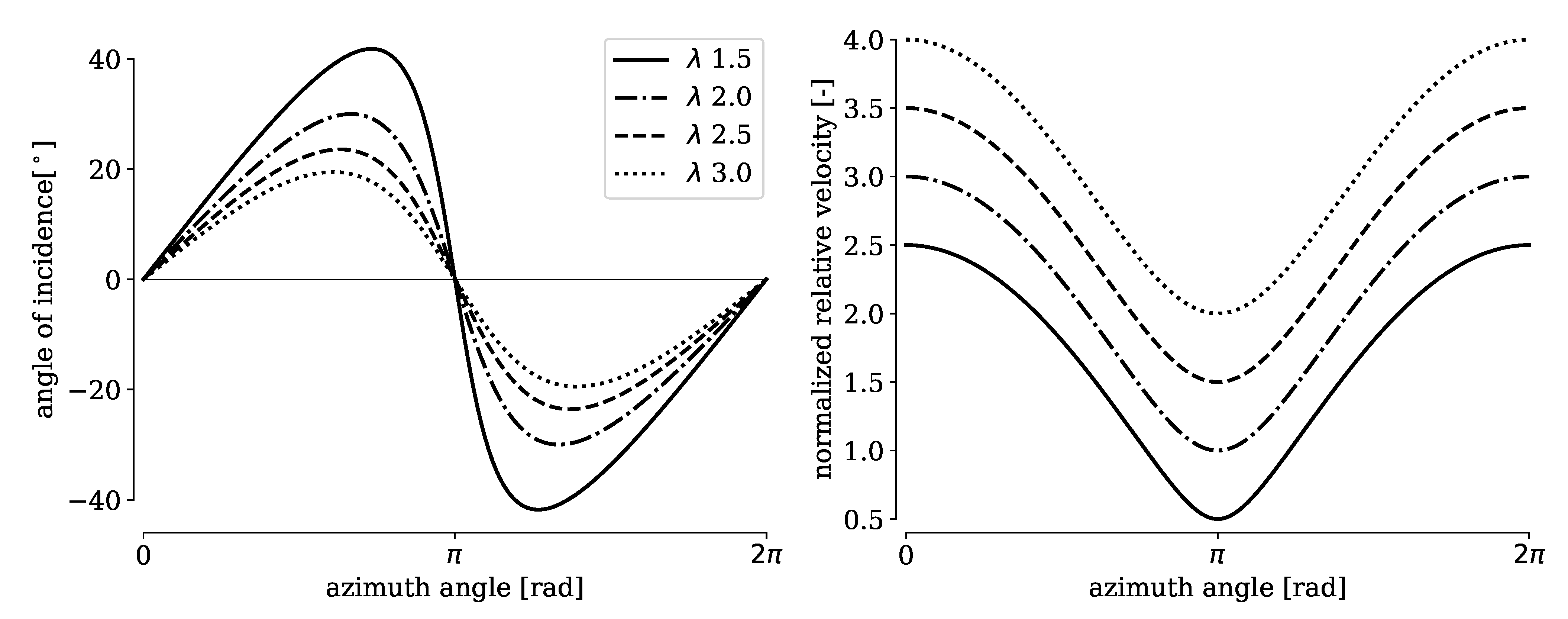
• a high solidity along with high tip-speed ratio will lead to strong blade-blade interaction. Blades then operate under unfavorable conditions, since the flow is not able to convect away the wake of the preceding blades;
• a low solidity along with low tip-speed ratio will lead to profile stall and poor efficiency, due to high angles of incidence and a low "harvesting" area of the rotor.

At the blade level, the flow can be characterized by two parameters linked to $\sigma$ and $\lambda$: The reduced frequency k and the trajectory of the angle of attack $\alpha$. While the latter expresses the operating point (see Equation (1)), k combines both $\sigma$ and $\lambda$ into one dimensionless parameter, as will be shown subsequently:

$$k=\frac{C·{\dot{\alpha }}_{\max }}{2v_{\infty }·{\alpha }_{\max }}=\frac{C·{\dot{\alpha }}_{\max }}{\omega ·2R·{\alpha }_{\max }}$$

(5)

Neglecting blade-blade interaction and downstream wake effects of the cross-flow turbine, the flow field of a CFTT at blade level can be investigated with a surrogate model consisting of an oscillating hydrofoil [26].

2. Experimental Model and Setup

In this case, the hydrodynamic profile will perform a pitch motion in accordance to the trajectory of $\alpha$ (see Equation (1)). An advantage of this setup is the simplification of the experimental setup and the focus on the blade itself. Since the experiment was conducted in a closed water tunnel at LEGI Labs Grenoble, the alternating relative flow velocity w was replaced by the constant inlet velocity $v_{\mathrm{ch}}$. This results in a constant Reynolds number, the effects of which on the results of this study are considered small. This comes along with a constant load and convection regime, which has to be considered for a transfer of the results to a real CFTT. The reduced frequency k for the given setup with constant $v_{\mathrm{ch}}$ and oscillation frequency $f_o$ can be found by combining Equation (5) (left) with the motion law for $\alpha$ (Equation (1)), its temporal derivative $d\alpha /dt$ and the definition of $\lambda$ (Equation (4)):

$$k=\frac{\pi ·f_o·C}{v_{\mathrm{ch}}·\left(\lambda -1\right)·arctan\left[{({\lambda }^2-1)}^{-\frac{1}{2}}\right]}$$

(6)

The most interesting feature of the deployed surrogate model is the ability to investigate a full set of turbine designs by variation of k and $\alpha$, according to Equation (6).

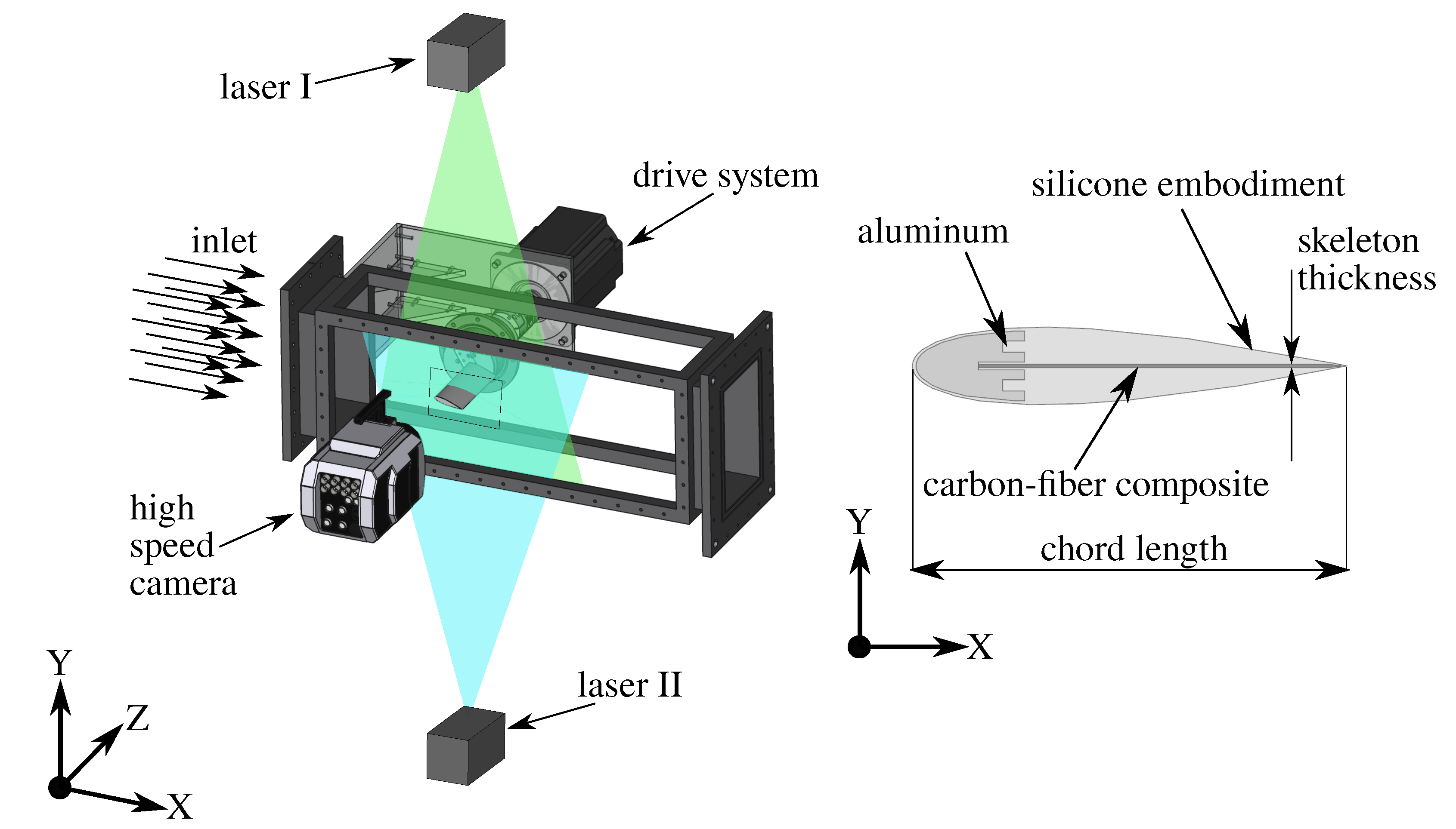
2.1. Experimental Facility

The water channel at LEGI Labs in Grenoble is operated in a closed loop with a maximum volume flow rate of 650 L/s at 20 m head. The facility is equipped with a test section of 1000 × 175 × 280 (L × W × H in [mm]), shown in Figure 3. The turbulence intensity in the core flow was measured to be 0.5% based on flow field measurements using laser Doppler anemometry (LDA). The minimum achievable inlet velocity is of 3 m/s due to instabilities in the volume rate and overheating of the pump drive for lower drive speed. Therefore, in the study at hand, the channel’s inflow velocity was set to 3.5 m/s.

2.2. Highly Flexible Hydrofoils

The adaptive blades were designed as a multi-material compound (see Figure 3). The first quarter of the profiles is milled from aluminum and considered to be rigid. The remaining parts comprise a composite skeleton built from a thin (0.3 mm) plate of carbon fiber embedded in an epoxy resin matrix and an embodiment of high flexible silicone. This design allowed for a variation of the profile stiffness by only changing the skeleton thickness. The chord length of 66 mm of the NACA0018-shaped hydrofoil led to a chord-based Reynolds number of about 250,000 for the inlet velocity $v_{\mathrm{ch}}$ = 3.5 m/s in the experimental setup.

A detailed description of the experimental facility, hydrodynamic load measurement, and flexible hydrofoils can be found in Hoerner et al., 2019 [24].

2.3. Pitch Motion Setup

A servo-drive system of 5 kW and 143 Nm peak torque is fed by a power inverter, allowing the realization of any arbitrary rotational motion. To this purpose, a drive communication software was customized (Abbaszadeh et al., 2019 [19]). During the experiments, the drive performs an oscillating pitch motion according to Figure 2, highlighting the case $\lambda$ = 2. This pitch motion leads, in addition to the main flow in the water channel, to a highly dynamic flow regime, comparable to the flow in the rotor of a single-bladed CFTT. The position feedback of the drive for one period, describing the evolution of $\alpha$, is shown along with the resulting flow field in Section 3.

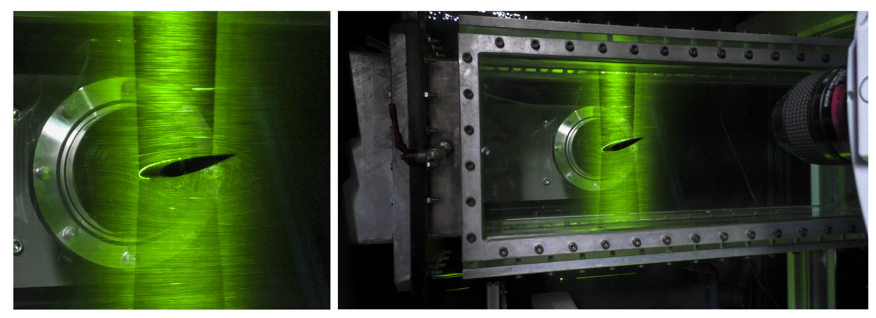
2.4. PIV Hardware Setup

The instantaneous flow field was captured with a time-resolved, two-dimensional, two-component (2D2C) PIV setup with 4 kHz temporal resolution (see Figure 3 and Figure 4). The light sheet of 2 mm thickness was built with two continuous lasers placed in parallel and pointing towards each other in the X-Y plane, in order to remove shadow effects from the hydrofoil. The plane was situated with a negative shift of 0.145 m in the Z-direction.

Both lasers were placed behind the test section: Laser I was equipped with an optical arm and a sheet generator which illuminated the measurement plane from the top, while Laser II generated the plane with a set of lenses from the bottom. The specifications of the lasers are given in

Table 1. Laser I and II specifications.

Spectra Physics Millenia
Wave length	[nm]	532
Type		continous NdYV04
Power	[W]	2 (pro 2 SJ)/5 (pro 5 SJ)

; both were set to 500 mW power. The high-speed camera, a Phantom V2511 (see

Table 2. High-speed camera specifications.

Phantom	V2511
Resolution	[px${}^2$]	1280 × 800	Pixel size	[$\mathsf{\mu }$m]	28
CMOS area	[mm${}^2$]	35.8 × 22.4	Color depth	[bit]	12
Focus	[mm]	105	Acquisition rate	[fps]	25,000

for specifications) covers an area of 120 × 74 mm${}^2$ with 1280 × 800 pixel at 12 bit gray-scale depth. The data was acquired with lens aperture of focus/4 and an exposure time of 50 $\mathsf{\mu }$s. Each recording consists of 16,500 frames, amounting to 4.125 s. The flow was seeded with silver-coated hollow glass spheres of 10 $\mathsf{\mu }$m diameter. The time synchronization of the position feedback and video recording is given by an external trigger signal from a pulse generator.

The PIV measurements were performed for a reduced frequency k = 0.24, represented by variations of the oscillation frequency $f_o$ = 2.25 Hz and a tip-speed ratio $\lambda$ = 2. This means that the flow field is dominated by a fully-dynamic stall regime. At first, measurements were performed for a rigid reference hydrofoil. Subsequently the experiment was repeated under exactly the same conditions for the flexible hydrofoil, which allows for a direct comparison of the influence of the passive stall control approach and consequences regarding the flow field.

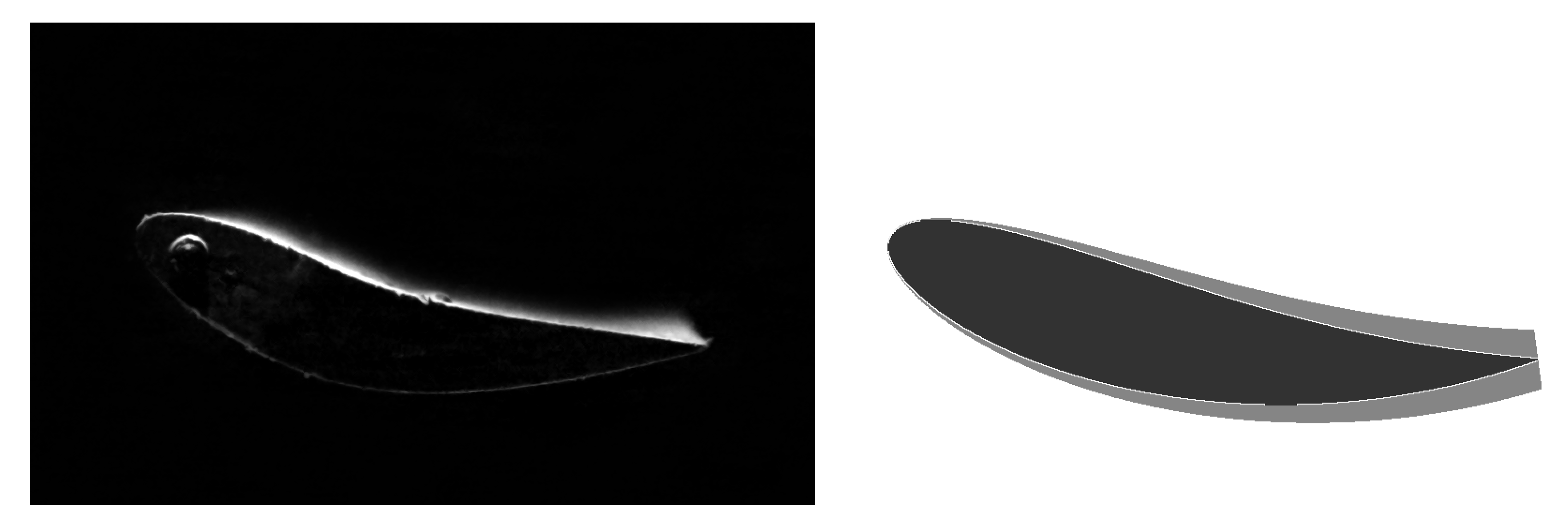
2.5. Preprocessing and Masking

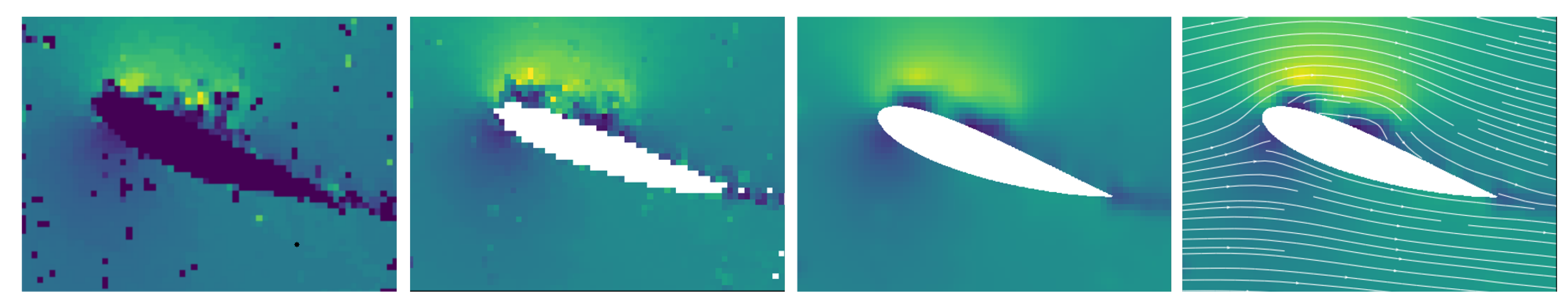
A particular challenge for the present study was the adhesion of particles to the silicone body, resulting in agglomerations on the surface. Reflections at the boundaries perturb the cross-correlation algorithm, so that the structure has to be masked. In the present case, the mask generation becomes a challenging task. The structure is in motion and simultaneously deforms, because the rigid body displacement is overlaid by an unknown and partly stochastic structural deformation. While the first can be easily predicted by the trajectory of the drive control or the position feedback, no reliable information is available for the deformation of the flexible body. To overcome this issue, a segmentation algorithm was developed to provide an adaptive mask for the PIV raw data. The algorithm and an additional technique used to measure cross-section deformation have been published as open-source code and are described in Hoerner 2020 [27].

The footage was taken by a camera perpendicular to the cross-section; therein, three-dimensional effects enlarge the projected area of the structure non-uniformly, as a result of non-uniform deformation of the hydrofoil itself across its span (in the Z-axis). This results in a sparser seeded (and hence darker) area, especially near the trailing edge. In consequence, a corrected mask (Figure 5), thicker than the NACA0018 geometry, was used during the PIV processing. This has a non-negligible effect on the measurements in the vicinity of the trailing edge and has to be considered in the evaluation of the results.

2.6. Processing

Fluidimage, a PIV processing framework introduced by Augier et al., 2019 [28] was utilized to perform the PIV processing of the raw data.

The process starts with image preprocessing and mask generation. The main processing (the cross-correlation) is performed in a multi-step setup, starting with an initial window size of 128 × 128 px${}^2$ and a final window size of 32 × 32 px${}^2$. In the current state only quadratic interrogation windows are supported by the software. The windows overlap of 50% leads to one vector for each 16 × 16 px${}^2$, or 1.5 × 1.5 mm${}^2$ respectively. A correlation peak value of 0.3 was chosen as a threshold during the multi-step process to ensure reliable results. All vectors obtained with lower correlation values were discarded and replaced by the output of a thin-plate-spline (TPS) interpolation algorithm. The continuous laser source and the high sample rate made for challenging conditions. Subsequent treatment methodology of the flow fields retrieved from the correlation was necessary and fully adapted to the data at hand.

2.7. Post-Processing

In a first step of data post-processing (see Figure 6), the (spatially) interpolated vectors (this is done by deploying thin-plate-spline radial basis functions during the processing in the Fluidimage software) for each time step with a correlation <0.3 were discarded and replaced by NaN (see Figure 6 (far left)). Resulting vector gaps were subsequently filled up, exploiting the high temporal resolution of the recordings to increase the reliability of the data. A time-based rolling average with a window of four frames replaced most of the removed vectors with reliable values from the neighboring time steps (see Figure 6 (center left)). To this effect, the average value of all available velocities in a given coordinate was calculated. NaN were sorted out before averaging over the remaining data points.

In the next step, a Gaussian filter was applied to the field. In order to work around remaining NaN in the velocity field, the filter was applied once for a field containing the NaN values, and once for a field with NaN replaced by zeros. The division of the second field by the first removes the influence from the zero velocities (see Figure 6 (right)). The resulting field does not contain the masked region, which is simply treated as a tracer-free region (set to ’0’) while processing the raw footage. A second, NACA0018 foil-shaped mask without thickened trailing edge, generated in parallel to the processing mask during the preprocessing, is superposed on the velocity fields for optical convenience. In the subsequent figures, except where explicitly mentioned, flow velocities v are shown as a dimensionless values after division by the average incoming flow speed ($v/\overline{v}$), and the color scale is constant, ranging from 0 $<v/\overline{v}<$ 2 for all subsequent velocity plots and videos.

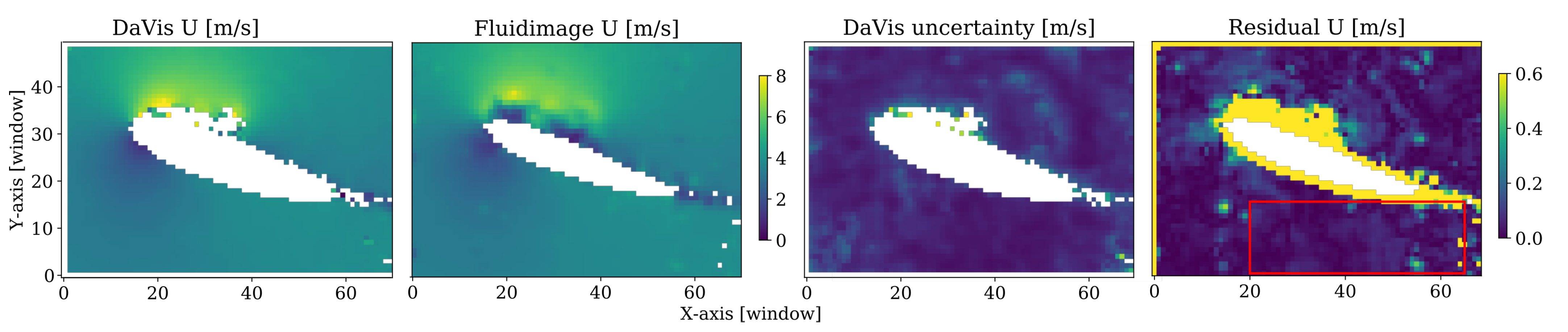
2.8. Uncertainty Estimation

An uncertainty estimation for PIV measurements is challenging, due to the high abstraction level of the method and the multitude of processing steps. In order to evaluate the reliability of results and in particular of Fluidimage, results were compared with those obtained from the commercial software solution DaVis, and by using its uncertainty estimation function. The same adaptive masks were used in both processes.

Table 3. DaVis and Fluidimage software settings used in the post-processing. Thin-plate-spline (TPS) stands for thin-plate spline interpolation.

	Davis		Fluidimage
Denoise	counts	1000	threshold	counts > 85%
	substraction
Vector calculation	time-series	multi-pass	time-series	multi-step
Window size/Steps	64 × 64	2	128 × 128	1
Overlap		0		50%
Smoothing	Gaussian weight	1:1	TPS
Correction	standard		correl < 0.3
Window size/Steps			64 × 64	1
Overlap				50%
Smoothing			TPS
Correction			correl < 0.3
Window size/Steps	32 × 32	2	32 × 32	1
Overlap		50%		50%
Smoothing	Gaussian weight	1:1	TPS
Correction	standard		correl < 0.3

shows the settings for the DaVis and Fluidimage software, which were chosen to be as similar as possible.

The results of the comparison are visualized in Figure 7 where all the fields are displayed in m/s. The left half shows the velocity fields retrieved from each of the two software solutions. The right half shows the uncertainty of the PIV measurement obtained from DaVis, which is mainly based on the correlation peaks of the cross-correlation. The rightmost image displays the difference between the two velocity fields. In Figure 7, it becomes visible that the two software packages have a different treatment of masks. Fluidimage sets the masked area to zero velocity. This results in a smearing of the boundaries and produces artificially low velocities at the boundaries of the hydrofoil. This effect is not visible for DaVis where the mask seems to be treated explicitly with more sophisticated methods. This increases the reliability of the velocity fields close to the mask boundaries. Such a specific boundary treatment is not implemented in Fluidimage at this stage.

The differences between both reconstructed velocity fields were evaluated on a smaller window (the red rectangle in Figure 7) in order to avoid unrepresentative differences resulting from the mask treatment. In this window, the maxima of the magnitude were found to be a +0.16 m/s and −4.04 m/s (an outlier). The average difference was about −0.02 m/s, which is less than 1% of the average flow speed.

A further error source is related to the drive system and the accuracy of the position control. The position feedback is retrieved from the power inverter with a set-point precision of 0.058° by 0.0439° resolver resolution. The zero angle was calibrated with 0.014° accuracy (0.25 mm per meter) with a precision leveling tool.

3. Results and Discussion

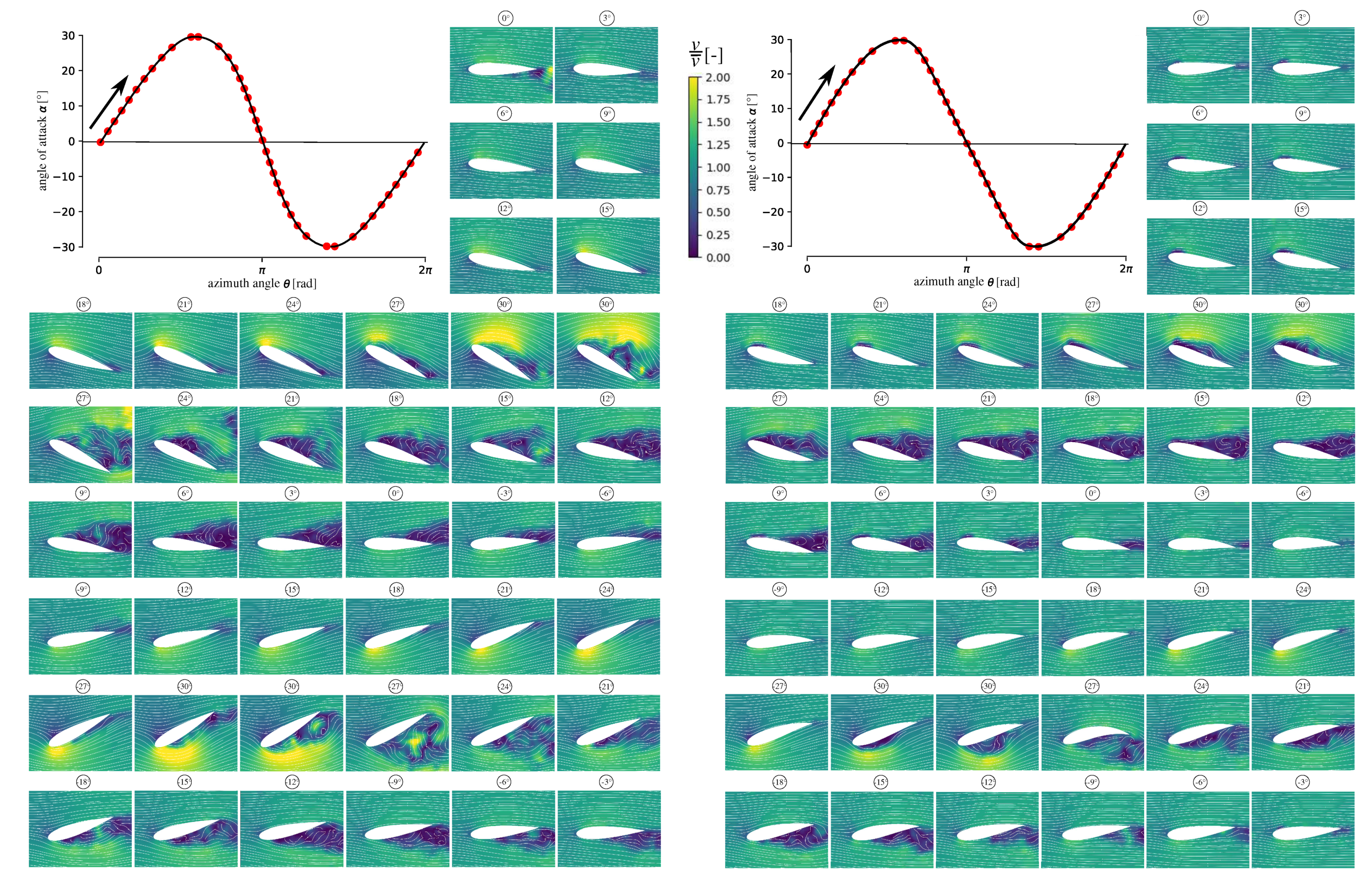
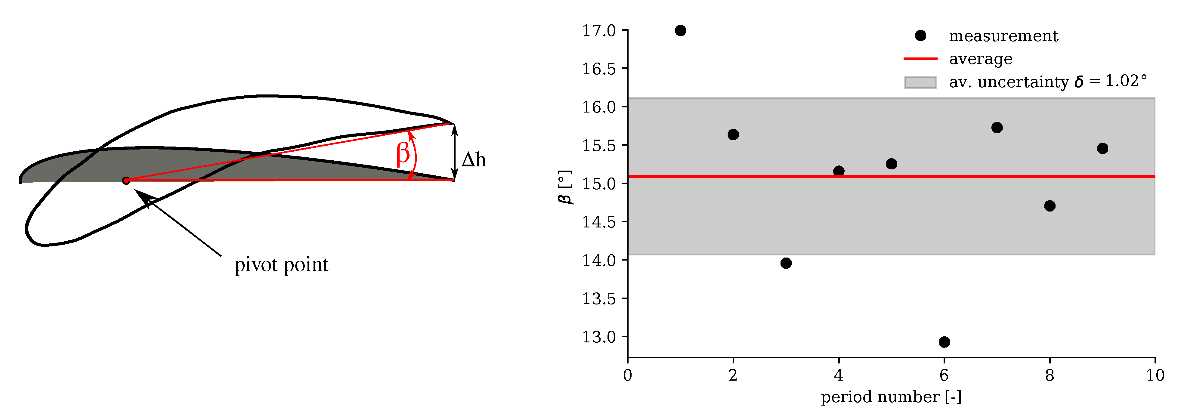
3.1. The Influence of the Flexibility on Profile Stall

A systematic description of the influence of the hydrofoil flexibility on the macroscopic flow field is obtained in this study. The high measurement uncertainty in the boundary layer (see Section 2.8) does not allow for investigations of the propagation of the boundary layer separation in detail, and so precise mechanisms of hydrofoil stall are not in the focus of the present investigations.

In Figure 8, a stepwise evolution of the flow field is shown in discrete steps of 3° for one period for rigid and flexible hydrofoil. Instantaneous velocity fields are presented. In the upper left diagram, the trajectory of the pitch motion (black line) is shown along with the angles (red circles) corresponding to the flow fields shown below. Starting with the rigid hydrofoil, the reference for a conventional CFTT, deep dynamic stall characteristics are found: the flow stays attached while passing through the static stall angle of $\alpha$ = 15° (NACA0018, Re = 230,000). The onset of flow separation can be observed on the trailing edge at $\alpha$ = 24°. The flow separation further grows and reaches its maximum, after passing ${\alpha }_{\max }$ = 30°, in the downward motion of the profile at $\alpha$ = 27°. Two counter-rotating vortices can be found in the wake structure. The size of the wake reduces as the angle of attack decreases. However, the flow remains detached until the hydrofoil gets in a clearly negative inclination ($\alpha$ = −6°), long after the static stall angle has been reached, the mark of a significant hysteresis. These effects are well described in literature as key characteristics of a dynamic stall regime (McCroskey 1976 [29]) and in former studies on pitching hydrofoils [30,31].

In the second half of the period, similar behavior can be reported (although some differences remain because the pitch velocity $\dot{\alpha }$ is higher in the downstroke). The largest profile wake zone appears again at $\alpha$ = −27°. The slower increase of the pitch angle allows for a faster reattachment of the flow ($\alpha$ = 3°). The hysteresis results in a regime where the flow only reattaches for very short parts of the oscillation period. This is in accordance to Gorle et al., 2016 [9] and their findings from PIV measurements on a four-bladed CFTT at $\lambda$ = 2 and k = 0.255.

The flow field of the flexible hydrofoil shows different characteristics. The structural adaptation to the flow leads to a significant decrease of the size of the wake, even though the flow separates again near $\alpha \approx$ 27°. The hysteresis effects reported for the rigid hydrofoil appear for the flexible hydrofoil as well. However, the detached flow phase remains shorter in the period. In the second half, the deformation increases, the hydrofoil tail flaps, while shedding a main vortex at $\alpha$ = −27° and the reattachment process is accelerated. This leads again to a shortened detached flow period. As shown in former studies, this structural adaptation and the resulting passive stall control leads to improved turbine efficiency [23,24]. The improvement is driven by drag reduction, which more than compensates for the reduction in lift resulting from the profile flexibility. The structural load also decreases because the structural deformation smoothens out the lift curves. This could translate into finer rotor geometries (reducing material usage) and longer lifetimes, due to decreased fatigue failure risks [24]. Beside this, a second, also remarkable point is the flow separation starting from the leading edge of the hydrofoil, which is a different behavior than observed for the rigid profile.

A chordwise flapping effect can be observed in the upwards motion from −12° to −6°, which is in accordance to the structural deformation measurements in a previous study [25,32]. This profile flapping is of stronger amplitude and can be linked to the shedding of the leading-edge vortex after convection of the profile, leading to significant deformations of the structure.

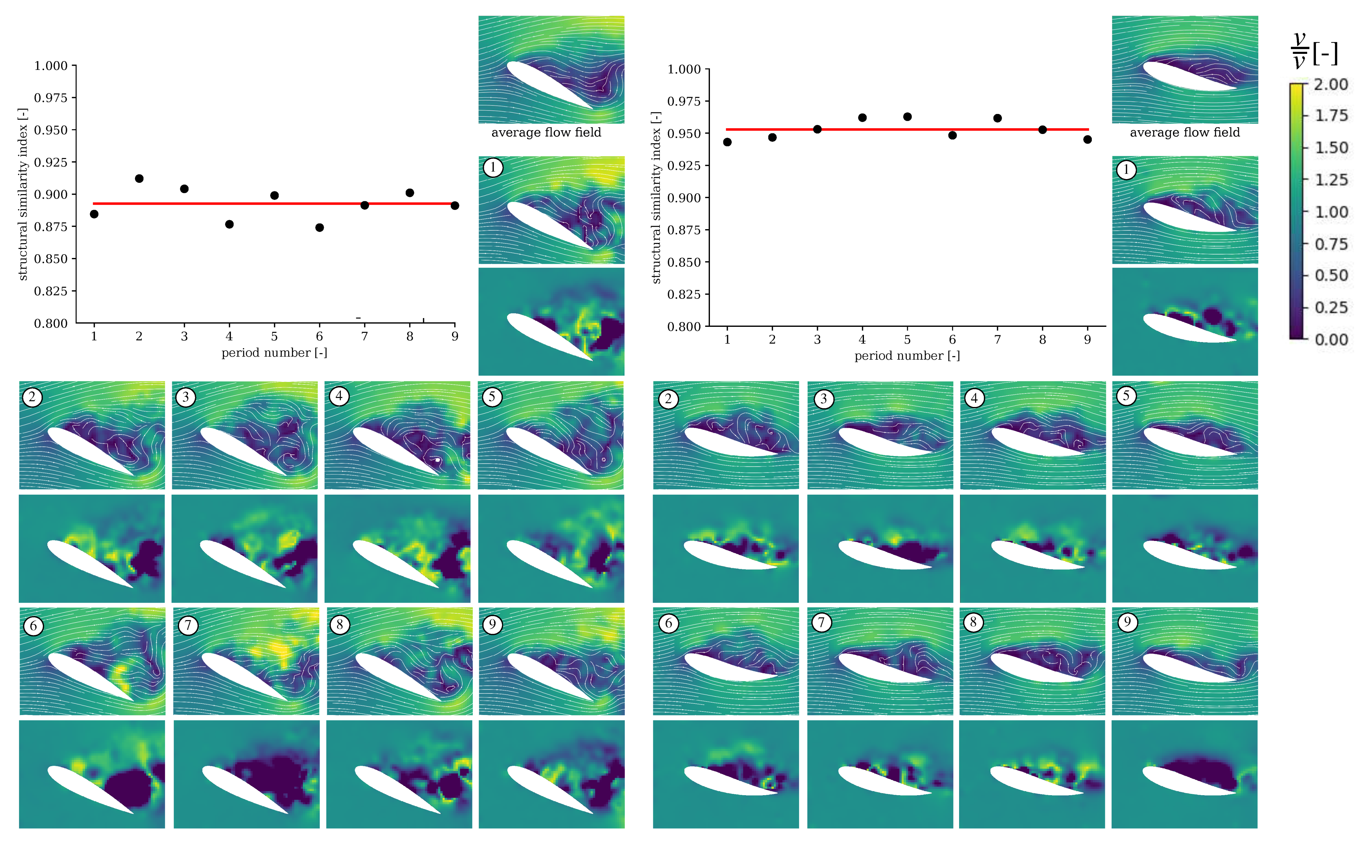
3.2. The Influence of the Profile Flexibility on the Periodicity of the Flow Field

The influence of the flexibility on the phase angle based periodicity, or reproducibility of the flow is also investigated. The chaotic component of the flow field is observed through a comparison of the instantaneous flow fields with the average field for any one foil position. A high similarity of the flow field between individual periods is a desirable property, and is, following a hypothesis of the authors, likely to correlate with higher efficiencies in farm configurations. In such installations, reducing turbulence in the wake of an individual turbine may improve conditions for downstream turbines, enabling an increase in the power of the complete array. In this case, it could be taken as a measure for the efficiency of the energy conversion process.

A meaningful comparison of any flow fields shall not focus on microscale differences, but instead observe similarities in the main flow structure. The structural similarity index (SSIM), as proposed by Wang et al., 2004 [33] is a suitable tool to express the similarity of two images by the evaluation of luminance, contrast and structural similarity. In the case at hand it allows for the comparison of the flow fields using a single, averaged index, based on macro-scale—structural—similarities of the fields. Therefore, this tool, originally developed to assess the quality of image compression tools, serves as a fast and robust method for an assessment of the periodicity of the flow and the information loss in a phase-averaged flow field.

Figure 9 shows this comparison of the flow fields in multiple stages once for the rigid (left) and once for the flexible profile (right). As an example, a fully-detached flow at $\alpha$ = 28° in the descending $\alpha$ motion is chosen using nine samples. The detached flow, a consequence of the dynamic stall regime induced by the periodic pitch motion, results in flow fields with significant stochastic properties. The number of periods for the set is limited to nine, due to the camera buffer size and the high sample frequency of the recording. However, this number of periods is sufficient to provide clear trends. The figure is divided in multiple sections. The averaged flow field is provided (top right) beside a diagram (top left) featuring the SSIM calculated between the instantaneous sample flow fields and the averaged one. Subsequently, pairs consisting of two images are shown: the instantaneous flow fields (numbered 1–9) and their difference relative to the averaged flow field (underneath). All velocity fields were initially uniformly scaled according to the averaged flow velocity $v_{\mathrm{ch}}$.

In the case of the rigid foil, on the left, the wake area accounts for a significant share of the region captured with PIV measurements. The averaging of the flow field obviously suppresses small-scale structures originating from the instantaneous flow fields. As expected, significant differences appear in the wake region of the flow field and feature high variations in magnitude, structure, and size. The SSIM varies with a range of 0.04 from 0.874 to 0.912 with an average value of 0.893, which shows the strong variations for this case.

The flow fields of the flexible hydrofoil are generally characterized by a smaller wake size and a less complex flow structure. This can be found by visual examination and is also expressed by the SSIM, which varies in a smaller range of 0.02 from 0.943 to 0.963, around the generally higher average of 0.953. This is a clear metric for a significantly higher periodicity of the flow. Exploiting the results of the segmentation algorithm deployed for the raw PIV footage masking, the deflection of the flexible hydrofoil is a second parameter in the assessment of the periodicity. Figure 10 shows the differences in-between the deflected inclination angles $\beta$ for the nine sample probes. The numbering of the periods is consistent with the numbering used in Figure 9. Variations of about 2° from the average can be reported. However, the bending characteristics are not correlated to the SSIM values. Further investigations of hydrodynamic loads and flow circulation around the profile could be appropriate in this case, but are out of the scope of this study.

4. Conclusions

A time-resolved 2D2C PIV study was performed on a hyperflexible pitching hydrofoil in a closed water tunnel.The open-source toolbox fluidimage and custom routines were deployed for post-processing the raw data after validation by comparison with a commercial reference code. This installation is deployed as a surrogate model for a CFTT. The flow field analysis allows for a clear description of the influence of the novel approach to deploy flexible turbine blades on CFTT. Furthermore, it provides a better understanding of the underlying mechanisms for these positive effects of passive flow control. The advantages of this model are the ability to closely investigate the CFTT rotor flow field at the blade level for multiple designs and operating points without hardware modifications. It could be shown that deployment of hyperflexible turbine blades attenuates the dynamic profile stall characteristics. This results in a smaller wake size during the fully stalled periods of a rotor revolution. Also, the periods of flow separation are shortened, which allows for a reduction of the drag and of the hydrodynamic loads. Chordwise flapping can be observed while the main vortex is shed after convection over the profile. In summary, it can be stated that the blade flexibility passively controls the flow by its adaptation. The hydrodynamic loads induce profile deformation, which reduces load peaks, ultimately leading to a damping of stall dynamics.

The flexibility of the blades is found to have significant effect on the structure of the wake. Beside a descriptive visual comparison of instantaneous and phase-averaged flow fields, the similarity between them was described quantitatively using the structural similarity index. The SSIM was found to be significantly higher (rising from 0.893 to 0.963) when using the flexible structure, showing fewer stochastic changes in wake features from period to period. This may be advantageous for farm installations.

In a parallel study using the same setup, surface tracking measurements were conducted; further work is intended to investigate the flow fields for multiple reduced frequencies and to link the results to the structural response and hydrodynamic loads. The effect of wake periodicity concerning energy harvesting will also be investigated in the future.

5. Materials

The data that supports the findings of the study are available from the corresponding author upon request.

References

1. Brownstein, I.; Kinzel, M.; Dabiri, J. Performance enhancement of downstream vertical-axis wind turbines. J. Renew. Sustain. Energy 2016, 8, 053306. [Google Scholar] [CrossRef]
2. Dabiri, J. Potential order-of-magnitude enhancement of wind farm power density via counter-rotating vertical-axis wind turbine arrays. J. Renew. Sustain. Energy 2011, 3. [Google Scholar] [CrossRef] [Green Version]
3. Whittlesey, R.; Liska, S.; Dabiri, J. Fish schooling as a basis for vertical axis wind turbine farm design. Bioinspir. Biomimetics 2010, 5, 035005. [Google Scholar] [CrossRef] [PubMed] [Green Version]
4. Jiang, C.; Shu, X.; Chen, J.; Bao, L.; Li, H. Research on Performance Evaluation of Tidal Energy Turbine under Variable Velocity. Energies 2020, 23, 6313. [Google Scholar] [CrossRef]
5. Shiono, M.; Suzuki, K.; Kiho, S. An experimental study of the characteristics of a Darrieus turbine for tidal power generation. Electr. Eng. Jpn. 2000, 132, 38–47. [Google Scholar] [CrossRef]
6. Paraschivoiu, I. Wind Turbine Design: With Emphasis on Darrieus Concept, 2nd ed.; Presses Internationales Polytechnique: Montréal, QC, Canada, 2002; ISBN 987-2-553-00931-0. [Google Scholar]
7. Laneville, A.; Vittecoq, P. Dynamic Stall: The Case of the Vertical Axis Wind Turbine. J. Sol. Energy Eng. Trans. ASME 1986, 108, 140–145. [Google Scholar] [CrossRef]
8. Ferreira, C.S.; van Kuik, G.; van Bussel, G.; Scarano, F. Visualization by PIV of dynamic stall on a vertical axis wind turbine. Exp. Fluids 2009, 46, 97–108. [Google Scholar] [CrossRef] [Green Version]
9. Gorle, J.; Chatellier, L.; Pons, F.; Ba, M. Flow and performance analysis of H-Darrieus hydroturbine in a confined flow: A computational and experimental study. J. Fluids Struct. 2016, 66, 382–402. [Google Scholar] [CrossRef]
10. Buchner, A.J.; Honnery, D.; Soria, J. Stability and three-dimensional evolution of a transitional dynamic stall vortex. J. Fluid Mech. 2017, 823, 166–197. [Google Scholar] [CrossRef]
11. Buchner, A.J.; Soria, J.; Honnery, D.; Smits, A. Dynamic stall in vertical axis wind turbines: Scaling and topological considerations. J. Fluid Mech. 2018, 841, 746–766. [Google Scholar] [CrossRef]
12. Miller, M.; Duvvuri, S.; Brownstein, I.; Lee, M.; Dabiri, J.; Hultmark, M. Vertical-axis wind turbine experiments at full dynamic similarity. J. Fluid Mech. 2018, 844, 707–720. [Google Scholar] [CrossRef] [Green Version]
13. Benton, S.; Visbal, M. The onset of dynamic stall at a high, transitional Reynolds number. J. Fluid Mech. 2019, 861, 860–885. [Google Scholar] [CrossRef]
14. Müller-Vahl, H.; Strangfeld, C.; Nayeri, C.; Paschereit, C.; Greenblatt, D. Control of thick airfoil, deep dynamic stall using steady blowing. AIAA J. 2014, 53, 277–295. [Google Scholar] [CrossRef]
15. Müller-Vahl, H.; Nayeri, C.; Paschereit, C.; Greenblatt, D. Dynamic stall control via adaptive blowing. Renew. Energy 2016, 97, 47–64. [Google Scholar] [CrossRef]
16. Lazauskas, L.; Kirke, B. Modelling passive variable pitch cross flow hydrokinetic turbines to maximize performance and smooth operation. Renew. Energy 2012, 45, 41–50. [Google Scholar] [CrossRef]
17. Khalid, S.; Liang, Z.; Sheng, Q.H.; Zhang, X.W. Difference between Fixed and Variable Pitch Vertical Axis Tidal Turbine—Using CFD Analysis in CFX. Res. J. Appl. Sci. Eng. Technol. 2013, 5, 319–325. [Google Scholar]
18. Mauri, M.; Bayati, I.; Belloli, M. Design and realisation of a high-performance active pitch-controlled H-Darrieus VAWT for urban installations. In Proceedings of the 3rd Renewable Power Generation Conference, Naples, Italy, 24–25 September 2014. [Google Scholar] [CrossRef]
19. Abbaszadeh, S.; Hoerner, S.; Maître, T.; Leidhold, R. Experimental investigation of an optimised pitch control for a vertical-axis turbine. IET Renew. Power Gener. 2019, 13, 3106–3112. [Google Scholar] [CrossRef]
20. Strom, B.; Brunton, S.; Polagye, B. Intracycle angular velocity control of cross-flow turbines. Nat. Energy 2016, 2, 1–9. [Google Scholar] [CrossRef]
21. Fish, F. Power output and propulsive efficiency of swiming bottlenose dolphins (tursiops truncatus). J. Exp. Biol. 1993, 183, 179–193. [Google Scholar]
22. Zeiner-Gundersen, D. A novel flexible foil vertical axis turbine for river, ocean and tidal applications. Appl. Energy 2015, 151, 60–66. [Google Scholar] [CrossRef]
23. MacPhee, D.; Beyene, A. Fluid–structure interaction analysis of a morphing vertical axis wind turbine. J. Fluids Struct. 2016, 60, 143–159. [Google Scholar] [CrossRef]
24. Hoerner, S.; Abbaszadeh, S.; Maître, T.; Cleynen, O.; Thévenin, D. Characteristics of the fluid—Structure interaction within Darrieus water turbines with highly flexible blades. J. Fluids Struct. 2019, 88C, 13–30. [Google Scholar] [CrossRef] [Green Version]
25. Hoerner, S.; Bonamy, C.; Cleynen, O.; Maître, T.; Thévenin, D. Darrieus vertical-axis water turbines: Deformation and force measurements on bioinspired highly flexible blade profiles. Exp. Fluids 2020, 61. [Google Scholar] [CrossRef]
26. Ly, K.; Chasteau, V. Experiments on an Oscillating Aerofoil and Applications to Wind-Energy Converters. J. Energy 1981, 5, 116–121. [Google Scholar] [CrossRef]
27. Hoerner, S. Characterization of the Fluid–Structure Interaction on a Vertical Axis Turbine with Deformable Blades. Ph.D. Thesis, University Otto-von-Guericke, Magdeburg, Germany, 2020. [Google Scholar] [CrossRef]
28. Augier, P.; Mohanan, V.; Bonamy, C. FluidDyn: A Python open-source framework for research and teaching in fluid dynamics by simulations, experiments and data processing. J. Open Res. Softw. 2019, 7. [Google Scholar] [CrossRef] [Green Version]
29. McCroskey, W.; Carr, L.; McAllister, K. Dynamic Stall Experiments on Oscillating Airfoils. AIAA J. 1976, 57–63. [Google Scholar] [CrossRef]
30. Ducoin, A.; Astolfi, J.A.; Sigrist, J.F. An experimental analysis of fluid structure interaction on a flexible hydrofoil in various flow regimes including cavitating flow. Eur. J. Mech. B/Fluids 2012, 36, 63–74. [Google Scholar] [CrossRef] [Green Version]
31. Ducoin, A.; Deniset, F.; Astolfi, J.A.; Sigrist, J.F. Computational and experimental investigation of flow over a transient pitching hydrofoil. Eur. J. Mech. 2009, 28, 728–743. [Google Scholar] [CrossRef] [Green Version]
32. Hoerner, S.; Bonamy, C. Structured-light-based surface measuring for application in fluid—Structure interaction. Exp. Fluids 2019, 60, 168. [Google Scholar] [CrossRef]
33. Wang, Z.; Bovik, A.C.; Sheikh, H.R.; Simoncelli, E.P. Image quality assessment: From error visibility to structural similarity. IEEE Trans. Image Process. 2004, 13, 600–612. [Google Scholar] [CrossRef] [Green Version]
Figure 1. Three-dimensional computer-aided design (CAD) model of a three-bladed H-Darrieus cross-flow tidal turbine (CFTT) and vorticity field from numerical investigations at tip-speed ratio λ = 2. CFTTs generate a complex flow field due to the cross-flow design and the lack of a guiding structure (Software package OpenFOAM/Paraview).
Energies 14 00797 g001
Figure 2. Alternating angle of incidence α (left) and relative velocity w (right) at blade level in dependence of azimuth angle θ and tip-speed ratio λ . The relative velocity w is normalized to the far-field velocity: w / v .
Energies 14 00797 g002
Figure 3. Experimental setup: (Left) The water tunnel test section is equipped with a servo-drive system allowing for a precise set-point control. A six-axis load cell captures the forces and moments acting on the profile. (Right) The stiffness of the flexible hydrofoils can be adjusted by the thickness of the carbon-fiber composite skeleton.
Energies 14 00797 g003
Figure 4. Setup of the two-dimensional, two-component (2D2C) particle image velocimetry (PIV) measurement with two synchronized lasers and high-speed camera at the LEGI labs closed-loop water tunnel. (Left) Detail of the inclined rigid hydrofoil, with flow separation. (right) The high-speed camera appears in the right of the image. Pathlines of particles are partly visible. Photos by Nicole Lambert, CNRS/LEGI 2017.
Energies 14 00797 g004
Figure 5. (Left) High-speed recording of the hydrofoil motion. The hyper-flexible hydrofoil encounters strong deformations for high angles of incidence. (Right) PIV mask generated from PIV raw data with thickened tail (grey) to cover three-dimensional deformation effects and recognized NACA0018 structure (black). The recordings belong to two different measurement campaigns.
Energies 14 00797 g005
Figure 6. Postprocessing corrections on the vector field: (far left) Raw flow field with magnitude of the pixel shift and empty spaces from low correlation (<0.3). (center left) Resulting field after application of the temporal rolling average with window size 4. (center right) final velocity field, after application of a Gaussian filter and calibration. (far right) Filtered vector field with streamlines: The velocity is displayed as non-dimensional velocity relative to the average flow speed v / v ¯ .
Energies 14 00797 g006
Figure 7. (Far left) Velocity field in m/s obtained by DaVis; (center left) Resulting field from Fluidimage with temporal rolling average with window size 4 and a Gaussian smoothing; (center right) Uncertainty of the PIV measurement in m/s from DaVis; (far right) difference between the magnitudes of the velocities from DaVis and Fluidimage, in m/s.
Energies 14 00797 g007
Figure 8. Flow fields for selected angles of incidence of one period of the oscillating pitch motion. The top-left diagram shows the pitch trajectory. The red points in the diagrams show the phase angle of the flow fields. (Left) Deep dynamic stall on a rigid NACA0018 hydrofoil at k = 0.24 for λ = 2 and σ = 1.5. Three-dimensional, chaotic structures with multiple, partly counter-rotating vortices are found in the separated zone. (Right) Flexible hydrofoil at k = 0.24 for λ = 2 and σ = 1.5.
Energies 14 00797 g008
Figure 9. Averaged flow field (top plot), instantaneous flow fields (numbered 1–9) and relative velocity difference to the average (underneath) around the rigid (left) and the flexible (right) hydrofoil for an identical angle of incidence in multiple periods ( α = 28°, k = 0.24). The diagrams show the structural similarity of the flow fields for each period.
Energies 14 00797 g009
Figure 10. Definition of β . The profile tip was not considered to suppress errors from tip recognition uncertainty in the cross-section detection algorithm. Flexible profile deformation for multiple periods, expressed with the deformed angle of incidence β ( α = 28°, k = 0.24).
Energies 14 00797 g010