Abstract
Assessing the efficiency of a tidal turbine array is necessary for adequate device positioning and the reliable evaluation of annual energy production. Array efficiency depends on hydrodynamic characteristics, operating conditions, and blockage effects, and is commonly evaluated by relying on analytical models or more complex numerical simulations. By applying the conservations of mass, momentum, and energy in an idealized flow field, analytical models derive formulations of turbines’ thrust and power as a function of the induction factor (change in the current velocity induced by turbines). This simplified approach also gives a preliminary characterization of the influence of blockage on array efficiency. Numerical models with turbines represented as actuator disks also enable the assessment of the efficiency of a tidal array. We compare here these two approaches, considering the numerical model as a reference as it includes more physics than the analytical models. The actuator disk approach is applied to the three-dimensional model Telemac3D in realistic flow conditions and for different operating scenarios. Reference results are compared to those obtained from three analytical models that permit the investigation of the flow within tidal farm integrating or excluding processes such as the deformation of the free surface or the effects of global blockage. The comparison is applied to the deployment of a fence of turbines in the Alderney Race (macro-tidal conditions of the English Channel, northwest European shelf). Efficiency estimates are found to vary significantly from one model to another. The main result is that analytical models predict lower efficiency as they fail to approach realistically the flow structure in the vicinity of turbines, especially because they neglect the three-dimensional effects and turbulent mixing. This finding implies that the tidal energy yield potential could be larger than previously estimated (with analytical models).
1. Introduction
The development and exploitation of low-carbon energies is essential to limit the impact of climate change. In Europe, ocean energy has attracted increasing interest, especially in the tidal energy sector, mainly as this resource is, among the different forms of marine energies, highly predictable [1]. A number of potential sites, with high resources, have been identified in northwest European shelf seas including the Alderney Race in the English Channel [2], the Pentland Firth in North Scotland (UK) [3], or the Fromveur Strait in western Brittany (France) [4]. Nowadays, several technologies have been tested on-site (e.g., HydroQuest, Simec Atlantis turbines, Sabella, etc.) and the tidal energy sector is currently planning the deployment of arrays able to produce dozens of MW.
Maximizing the potential output of tidal turbines requires, however, an optimal positioning of devices. The design of array has therefore attracted the interest of numerous research studies relying either on lab-scale experiments or analytical and/or numerical models. Those investigations integrate, most of the time, methodologies and concepts initially developed for wind turbines. Beyond changes in fluid density, a great difference between the exploitation of wind and tidal current is that tidal currents are constrained vertically by the free surface. This constriction of the tidal flow significantly influences the turbine performances and is referred to as blockage effect.
A series of analytical models were developed to investigate the blockage effect on turbines’ performance. These effects were studied by Garrett and Cummins [5] who applied the theory of Lancaster–Betz to a constrained flow with a blockage ratio ε (i.e., the surface swept by the blades over the cross-sectional area of the flow). They demonstrated that, in comparison to a turbine operating in an unconstrained stream (which is the case in the Lancaster–Betz theory), the maximum power extractable by a turbine (known as the Lancaster–Betz limit) varies as a function of (1 − ε)−2, thus exhibiting the increase of this maximum power with the blockage ratio. Whelan et al. [6] then modified this model by integrating the change in water depth caused by the turbine operation. In addition, Nishino and Willden [7] used the analytical model of Garrett and Cummins [5] to investigate the flow through and around a fence of devices arrayed across part of a wide channel cross section.
However, whereas analytical models permit the estimation of turbines’ performance, they rely on simplified configurations (idealized geometry), schematic turbine representation (e.g., swirl neglected), and simplified physics (e.g., quasi-inviscid flows). Numerical models are therefore useful to estimate array efficiency under more realistic flow conditions. This can be achieved with sophisticated blade-resolved models [8], blade element momentum theory [9], or vortex models [10], but also with more simplified turbine representation based on the actuator disk (AD) concept. This modelling approach consists of representing individual turbines as disks that apply the thrust experienced by turbines on the fluid. It is achieved by integrating in the momentum equation a sink term applied over the disks’ area. The AD method was validated with different lab-scale experiments, thus confirming its ability in simulating far turbine wakes [11]. It was therefore integrated in regional hydrodynamics models to perform wake-field studies under realistic sea conditions. Hence, Michelet et al. [12] applied the AD method in the regional ocean modelling system (ROMS [13]) to analyze the influence of the tidal asymmetry on the power output of an array of eight turbines deployed in the Fromveur Strait (western Brittany, France). By applying such an approach, Nguyen et al. [14] highlighted the effect of the flow rectilinearity on the power output of an array deployed in the Alderney Race (English Channel); and Thiébot et al. [15] demonstrated the influence of the wake-added turbulence on the power production of an array containing up to thirty devices.
In the present contribution, we investigate the efficiency of a fence of turbines deployed in the Alderney Race (in the English Channel between Alderney Island and the Cap de la Hague, France) by comparing predictions from (i) a series of analytical models and (ii) a reference regional simulation in which tidal turbines are represented by ADs. In addition to obtaining refined estimates of array efficiency, the objective is to provide further insights about these different approaches for advanced resource assessments in potential tidal stream energy sites. Indeed, analytical models constitute fast and simple approaches of tidal array efficiency, particularly useful in the preliminary stages of a tidal farm project, thus sparing time-consuming computational resources. However, these simplified approaches integrate increased uncertainties with respect to more realistic numerical simulations liable to encompass the complex coastline geometry, bathymetric features, hydrodynamic forcings, and associated spatio-temporal variability, as well as the potential interaction of turbine wakes within the array. It appears therefore fundamental to assess the discrepancy between analytical models and an advanced numerical simulation.
2. Materials and Methods
2.1. Site Description—Scenarios of Tidal Stream Energy Extraction
The site retained for this study is the Alderney Race, which is a progressive wave system. The high tidal current magnitudes of the site result from the combination of extreme tidal ranges in the southern part of the English Channel (exceeding 14 m near Mont Saint Michel) and a constriction (bottleneck effect) of the flow between the Cap de la Hague (France) and the island of Alderney. With current magnitude exceeding 5 m/s and depth suitable to deploy tidal turbines, this 15 km wide strait is one the most promising sites for tidal stream energy exploitation in the world [2]. Numerous investigations have therefore been performed to assess the potential annual energy production of the site, with the most optimistic estimates exceeding 10 TWh/year [16,17,18].
This study is an extension of previous investigations conducted on the same area of the Alderney Race with Telemac3D [19]. Thus, we rely on the model configuration implemented by Thiébot et al. [15] and focus on the same period (corresponding to a mean spring tide). However, we consider another way to analyze the array efficiency (described in Section 2.3) and we consider a different scenario of turbine deployment (different number of turbines and arrangement). Figure 1a shows the location of the study zone. Time-series of current magnitude and direction and free surface elevation (Figure 2) have been extracted in the center of the study zone at the point of coordinates (49°42.300′ N; 2°6.180′ W). Times of peak ebb and flood retained to assess the array efficiency are extracted from the time series of current magnitude at the center of the fence of turbines. The corresponding current velocity directions are represented in Figure 1b,c.
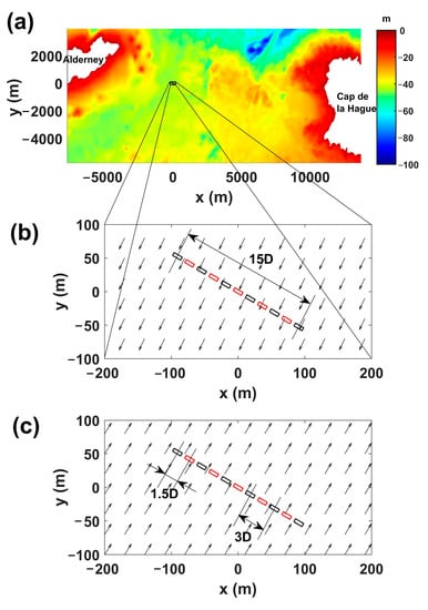
Figure 1.
(a) Bathymetry of the study site with location of the fence of turbines. Depth-averaged current direction during peak (b) ebb and (c) flood of a mean spring tide. The lateral spacing (center to center) are indicated in number of turbine diameters D. For a lateral spacing of 1.5D, 11 turbines are active. For a lateral spacing of 3D, only the 6 turbines represented in black are active. The origin of the coordinates system (in meters) corresponds to the center of the fence of turbines (49°42.300′ N; 2°6.180′ W).
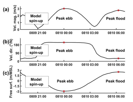
Figure 2.
Time-series of (a) depth-averaged velocity magnitude, (b) depth-averaged velocity direction, and (c) free surface elevation extracted from the Telemac3D model (simulation without turbine) in the center of the fence (49°42.300′ N; 2°6.180′ W). The red circles show times of peak ebb and flood retained to assess the array efficiency.
With regards to the scenarios of tidal stream energy extraction, we have considered a single fence of 14 m diameter turbines oriented perpendicularly to the predominant flow (Figure 1b,c). The turbine diameter is consistent with the value retained in [15]. It is worth noting that larger rotors could be used at this site, given that the depth exceeds 40 m. The hub height is 15 m. The length of the fence is 15D (distance between the axis of the turbines placed on the sides of the fence with D the turbine diameter, Figure 1b). Two lateral spacings between turbines, noted Δ, have been tested: 1.5D and 3D (Figure 1b,c), which leads to two different blockage ratios. The number of turbines when Δ = 1.5D and 3D, is 11 and 6, respectively (Figure 1b,c). Characteristics of the flow in peak ebb and flood are synthesized in Table 1. It is noteworthy that the Froude number, which is an input parameter of the analytical model of Whelan et al. [6], differs between peak ebb and flood as both water depth and current magnitude vary between the two tidal periods (Figure 2 and Table 1).

Table 1.
Characteristics of the flow during peak ebb and flood in the center of the fence (49°42.300 ′N; 2°6.180′ W) without the effects of turbines. Δ corresponds to the lateral spacing between devices (1.5D or 3D). The blockage ratio is equal to the surface area swept by the blades ( ) divided by the cross-section of the flow, that is to say the water depth multiplied by the distance between two consecutive turbines (1.5D or 3D).
2.2. Analytical Models
Analytical models intend to predict, for different values of velocity reduction (caused by the turbines), the efficiency of arrays. The efficiency is expressed in terms of thrust and power . For a single turbine, the thrust and power are given by Equations (1) and (2). The velocity reduction caused by the disk is expressed with an induction factor , Equation (3).
where (which is assumed to be constant and equal to 1025 kg/m3 for the present purpose) is the fluid density, and are the thrust and power coefficients, is the area swept by the turbines’ blades, is the velocity in the unperturbed flow (in a region of the flow that is not affected by the turbine), and is the velocity in the disk.
Analytical models rely on the linear momentum actuator disk theory (LMADT). In this theory, the effect of the turbine on the flow is represented by a change of pressure equal to . The LMADT consists of using the conservation of mass, momentum, and energy along the longitudinal axis of the turbine to derive relationships between the induction factor and the thrust and power coefficients. The LMADT leads to the famous Lancaster–Betz limit, which indicates that the maximum power coefficient value is 16/27 ≈ 0.59. The Lancaster–Betz model relies on equations that are valid in unbounded flows. However, for tidal turbine applications, the flows are bounded laterally and vertically. Hence, Garrett and Cummins [5] adapted the LMADT to model the horizontal flow through and around a tidal turbine deployed in a channel of finite dimensions (Figure 3(a1)). To this end, they applied the LMADT along the turbine’s axis and in the bypass flow (the accelerated flow around the turbine). They considered a quasi-inviscid flow with simplified velocity distribution: the velocity is thus supposed to be uniform in the bypass flow and in the stream tube passing through the turbine. Their model, noted G&C2007 in the following, permitted them to show that the Lancaster–Betz limit could be exceeded by a factor of (1 − ε)−2. Whelan et al. [6] rewrote the system of equations of G&C2007 and applied them to model the flow within a vertical plane passing through the turbine (Figure 3b). In doing so, they integrated the effect of the change in depth caused by the turbine (the rise of the free surface upstream of the turbine and drop of the free surface downstream of the turbine). Beyond confirming the effect of the blockage ratio, this new model, hereinafter denominated W2009, exhibited an increase in the extracted power with the Froude number. G&C2007 and W2009 were initially designed to analyze the performance of a single turbine in a channel. Nevertheless, those models are also applicable to multiple turbines spanned uniformly over the entire cross-section of a channel (as represented in Figure 3(a2) for G&C2007). However, in real-life applications, turbines are unlikely to be deployed over the entire channel cross-section because of either environmental and/or regulation constraints. Hence, Nishino and Willden [7] developed an analytical model, denoted N&W2012, to analyze the performance of a fence of turbines blocking partially a channel (Figure 3c). N&W2012 applied the G&C2007 model at two spatial scales: (i) at the “array scale” to analyze the flow through and around the fence of turbines, and (ii) at the “turbine scale” to analyze the flow through and around each turbine. For the present purpose, these three analytical models (G&C2007, W2009, and N&W2012) have been coded in Matlab in order to obtain, under the flow conditions synthetized in Table 1, the relationships between the power coefficient , the thrust coefficient , and the induction factor . The results are presented and discussed in Section 3.
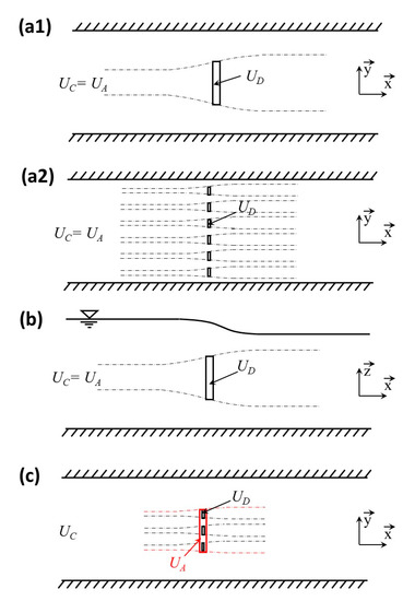
Figure 3.
Schematic representation of the analytical models. (a1) G&C2007 applied to a single turbine, (a2) G&C2007 applied to a fence of turbines arrayed uniformly across the channel, (b) W2009, and (c) N&W2012. (c) The dashed red curves represent the stream tube passing through the fence of turbines (surrounded by a red rectangle), and represent the flow at the “array scale”. The dashed black curves represent the stream tube passing through each turbine, and represent the flow at the “turbine scale”. is the velocity in the disk, is the velocity at the fence, and is the channel cross-sectional average of the streamwise velocity.
2.3. Numerical Model
The numerical model retained for analyzing the performance of the fence of turbines relies on the Telemac3D configuration of Thiébot et al. [15,20]. The mesh contains 16.8 million nodes. The horizontal cell size varies from 10 km (near the boundaries of the computational domain covering the English Channel) to 1 m in the zone occupied by the turbines. Vertically, the domain is discretized using 40 equally spaced horizontal planes (sigma-transformation), leading to a 1 m resolution in the zone occupied by the turbines. The turbulence is modelled with a k-ε closure scheme assuming an isotropic turbulence hypothesis. The model is forced by 11 tidal constituents. The regional model performance (simulations without turbine) has been validated with five acoustic doppler current profilers (ADCP) deployed in the waters of Alderney and demonstrated excellent model performance, with root mean square errors on the depth-averaged current velocities smaller than 0.2 m/s for four of the five ADCPs. The seabed morphology in the zone surrounding the turbines is featureless and flat with negligible variations of current velocities along the fence of turbines. The standard deviation of the velocity magnitude at the locations of the 11 turbines (case with Δ = 1.5D) is smaller than 0.01 m/s. The hydrodynamic conditions retained for the numerical model are thus similar to those retained in the analytical models (where the currents are uniform across the fence of turbines).
The turbine representation relies on an actuator disk (AD) formulation, which consists in applying, in the zone occupied by the turbines, a momentum sink term calculated from the thrust of the turbines. In our model, instead of computing the thrust from an upstream velocity (as in Equation (1)), it is evaluated from the velocity in the disk and a resistance coefficient (4) [21]. A first way to apply such AD formulation consists of setting the value of so that it corresponds to a given thrust coefficient value. For instance, in [15], the value of , which corresponded to , and was computed without blockage correction with Equations (5) and (6). For the present purpose, we apply the AD formulation in another way. Rather than setting a priori the value of (or ), we analyse the array efficiency under varying operating conditions (varying induction factors). To this end, we adopt the methodology of Nishino and Willden [22] which consists of performing a series of simulations with increasing values of momentum loss factor (=1, 2, …, 5) and then establishing, for different values of , the relationships between the thrust and the power coefficients and the induction factor with Equations (7)–(9).
where indicates the spatial average over the disk and is the current velocity in the unperturbed flow (determined from a simulation without turbine).
3. Results and Discussion
3.1. Results Overview
Figure 4 shows estimates of thrust and power coefficients with respect to the induction factor for the two array configurations (lateral spacings of 1.5D and 3D), the three analytical models (G&C2007, W2009, and N&W2012), and the reference Telemac3D simulations with AD. These results are represented at peak ebb and flood of the mean spring tide shown in Figure 2.
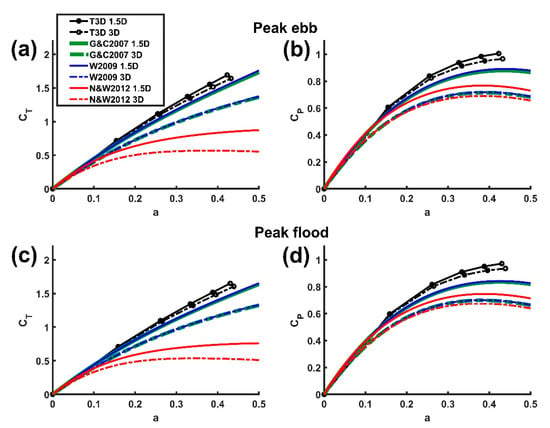
Figure 4.
Thrust (a,c) and power (b,d) coefficients as a function of the induction factor. Estimations are shown at peak (top) ebb and (bottom) flood of the mean spring tide represented in Figure 2.
3.2. Inter-Comparison of Analytical Models
Firstly, whatever the model retained, peak ebb flow conditions lead to greater thrust and power coefficients than peak flood conditions. The thrust and the power coefficients are 4.3% and 1.1% greater during peak ebb than peak flood (those values are given for = 1/3 and are averages of all model results). This appears related to a greater blockage ratio (Table 1). Indeed, in the Alderney Race, the peak ebb corresponds approximately to low tide (Figure 2) and the blockage ratio is thus greater (as the cross-section reduces). Secondly, for the same reason (difference in blockage ratio), it is also observable that a lateral spacing of 1.5D (continuous lines) gives greater thrust and power than a lateral spacing of 3D (dashed lines). Thirdly, with regards to the inter-comparison of analytical models, we can see that the predictions of G&C2007 and W2009 are nearly similar, with slightly greater values predicted by W2009. The difference in efficiency is very small because, in the tested conditions, the Froude numbers are small (in comparison with the value of 0.22 retained in [6]). Fourth, N&W2012 predicts lower performance than the two other analytical models (−6.8% for the power coefficient at = 1/3; this value is an average of the peak ebb and peak flood conditions). This may be because it considers the flow at both the array and the turbine scales, while G&C2007 and W2009 only consider the turbine scale. To explain in more detail the difference between the three analytical models, we rely on the notations of [7] with the velocity in the channel, the velocity in the array, and the velocity in the disks (Figure 3). In G&C2007 and W2009, only the turbine scale is accounted for and the array-scale effect is neglected (i.e., the global effect of the turbines does not modify the flow passing through the fence). Thus, it is hypothesized that the velocity at the channel inlet is similar to the velocity upstream of the array (i.e., ) and the results of G&C2007 and W2009 are given in terms of local induction factor and local power and thrust coefficients and . In N&W2012, the thrust and the power result from (i) the local reduction of the velocity at the turbine scale (characterized by an array induction factor ), but it also integrates (ii) the reduction of the velocity upstream of the array due to the array-scale effect (characterized by an array induction factor ). The relationships between the local coefficients (used in G&C2007 and W2009) and the global coefficients (used in N&W2012) are therefore presented in Equations (10) and (11) [7].
As is smaller than 1, the efficiency estimates given by N&W2012 are smaller than those given by G&C2007 and W2009, which explains the differences between the three analytical model results shown in Figure 4.
3.3. Comparison between Analytical and Numerical Models
The numerical model predicts a higher efficiency than the analytical models (+22.1% for the power coefficient for = 1/3; this value is an average of the peak ebb and peak flood conditions). It is an important (and encouraging) finding. Indeed, it suggests that historic energy yield estimates based on analytical models are under-estimated and that the yield potential could be greater than previously estimated. Furthermore, the effect of the lateral spacing on the thrust and power differs between analytical and numerical models. Whereas Telemac3D predicts a slight gain in power coefficient when densely packing turbines (+3.4% when = 1/3), the analytical models predicts a much higher gain (+18.3%, +18.9%, and +10.5% for G&C2007, W2009, and N&W2012, respectively). These results exhibit that analytical and numerical models give significantly different efficiency estimates; and that they are characterized by different sensitivities to the blockage ratio. We suggest that mixing effects may play a role in such differences. Indeed, whereas analytical models assume that the viscous and turbulent mixing takes place only downstream of the location where the pressure equilibrates, the numerical model with AD simulates more realistically the mixing effects [22]. In the area surrounding the turbines, the wake-added turbulence (taken into account in the numerical model with AD) is expected to accelerate the flow in the wake of the turbines and reduce the flow in the bypass (horizontally and vertically). The effect of the mixing can be seen in Figure 5 and Figure 6 that show that rather than observing distinct regions with homogeneous velocity distributions (decelerated flow behind the turbine and accelerated flow around the turbines), the flow structure is much more complex. Indeed, in the wakes of the turbines, the velocity distribution is non-uniform with a maximal velocity reduction along the turbine axis; and a velocity deficit that enlarges progressively (while reducing in magnitude) and extends over a large section of the flow. These figures show furthermore that the flow behavior clearly differs under and above the device, which indicates that the flow is three-dimensional. Indeed, there are reduced velocity magnitudes near the seabed (and a high level of turbulence, which is not shown here) and a higher current speed near the free surface (and a lower level of turbulence). The figures suggest therefore that the idealized flow configuration retained by analytical models (Figure 3), where the velocities are supposed as uniform (in the wake and the bypass), may not apply in the present flow configurations and array arrangement.
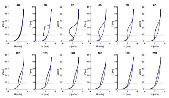
Figure 5.
Vertical distribution of the velocity magnitude at different positions along the wake of the turbine located in the middle of the fence (sixth turbine from the left for Δ = 1.5D and third turbine from the left for Δ = 3D, Figure 1b,c). Blue lines represent the simulations without turbines. Black lines represent the simulations with turbines. Continuous and dashed lines correspond to a lateral spacing of 1.5D and 3D, respectively. The horizontal lines indicate the top and the bottom of the turbines. The velocities have been extracted, at peak flood tide, from the simulation with AD and = 3 ( = 0.33 and 0.34 for Δ = 1.5D and Δ = 3D, respectively).
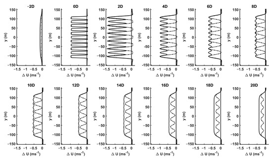
Figure 6.
Horizontal distribution of the velocity deficit (velocity magnitude with turbines minus velocity magnitude without turbines) at the hub height (15 m above the flat seabed) at different streamwise positions from the fence of devices. Continuous and dashed lines correspond to a lateral spacing of 1.5D and 3D, respectively. The velocities have been extracted, at peak flood tide, from the simulation with AD with = 3 ( = 0.33 and 0.34 for Δ = 1.5D and Δ = 3D, respectively). The orientation of the axis differs from that retained in Figure 1.
The discrepancies between the analytical and numerical models (Figure 4) is smaller for a lateral distance of 1.5D (continuous curves) than for a lateral spacing of 3D (dashed curves), which suggests that analytical models are more reliable when blockage ratios are large. To understand why, we now compare the flow field around the turbines for both a lateral spacing of 1.5D and 3D. Firstly, with regards to wake-added turbulence, the comparison of dashed and continuous lines in Figure 7 highlights a greater level of turbulent kinetic energy behind the fence when the lateral spacing is 1.5D (because there are more turbines producing turbulence along the fence). There is therefore more mixing when the lateral spacing is 1.5D. As analytical models neglect turbulence, their performance should be worse for Δ = 1.5D than for Δ = 3D. As the contrary is found, the wake-added turbulence may not be responsible for the difference of performance between Δ = 1.5D and Δ = 3D. Secondly, we compare the vertical distribution of the current magnitude, which shows limited differences between the two cases as shown in Figure 5 (by comparing dashed and continuous lines). Thirdly, we investigate the difference in the spatial distribution of horizontal velocity deficit (Figure 6), which shows a contrasted flow structure for the two cases (Δ = 1.5D and Δ = 3D). Indeed, for the lateral spacing of 3D, the turbines behave nearly independently with wakes surrounded by slight flow acceleration (negative velocity deficit between the turbines). Whereas for the lateral spacing of 1.5D, the turbines are so close to each other that they behave as a whole, with nearly no flow acceleration between the turbines and a noticeable flow deceleration upstream of the turbines (Figure 6, position = −2D). This flow field should be more in line with the idealized flow predicted by analytical models. We thus think that analytical models perform better for great blockage ratios because they approach more realistically the horizontal distribution of the current velocities under such conditions. Nevertheless, although this comparison (1.5D vs. 3D) suggests that analytical models are more reliable for great blockage ratios, additional investigations on a wider range of scenarios is required to generalize this result and to find the flow conditions under which analytical models may be applicable.
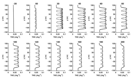
Figure 7.
Horizontal distribution of the turbulent kinetic energy (TKE) at the hub height (15 m above the flat seabed) at different streamwise positions from the fence of devices. Continuous and dashed lines correspond to a lateral spacing of 1.5D and 3D, respectively. The values have been extracted, at peak flood tide, from the simulation with AD with = 3 ( = 0.33 and 0.34 for Δ = 1.5D and Δ = 3D, respectively). The orientation of the axis differs from that retained in Figure 1.
4. Conclusions
In order to maximize the production of a tidal array, it is necessary to (i) select a site with high tidal resources and (ii) assess the efficiency of the array under different flow and operating conditions. Considering an application in the Alderney Race, we have compared the efficiency estimates given by three different analytical models and a numerical model in which turbines have been represented by actuator disks.
The inter-comparison of the analytical models showed that in addition to the turbine-scale effect, which controls the modification of the flow velocity near the turbines, the array-scale effect, which controls the modification of the flow through and around the array, has a strong detrimental effect on the array efficiency. Indeed, the model developed by Nishino and Willden [7] predicts much lower efficiency estimates than models that focus solely on the turbine-scale effect (the models of Garrett and Cummins [5] and Whelan et al. [6]). The model of Nishino and Willden [7] contains more physics than the two other models (that neglect the array scale). Thereby, it should give more reliable efficiency estimates. However, the agreement with the results of the reference (numerical) model is poorer. Thus, we expect that the better agreement by the models that neglect the array scale is an artefact. Indeed, neglecting the array scale tends to overestimate the farm efficiency, which may fortuitously reduce the gap between the analytical model and the reference model.
The efficiency estimates obtained from analytical models have been compared to those obtained from a three-dimensional Telemac3D model including actuator disks. Although actuator disks do not contain all the physics to be fully representative of real turbines, they should give a more representative description of the flow within the array than analytical models as they consider the three-dimensional characteristics of the flow and include the mixing caused by the wake-added and ambient turbulence. The comparison between analytical and numerical models suggests that, in the tested flow conditions and scenario of tidal stream energy extraction, analytical models highly underestimate the array efficiency, especially when the blockage ratio is low. It implies that historic tidal energy yield estimates relying on analytical models may be under-estimated. Finally, beyond the comparison between analytical and actuator-based models, it is important to remember that very few tidal turbines have been tested on-site and that no turbines have been tested in the Alderney Race, yet. Therefore, there is no reliable references to validate the efficiency estimates given by actuator disks. Additional investigations are thus requested to estimate the uncertainties in energy yield estimates and to determine whether (or not) a higher complexity of models is needed to obtain reliable efficiency estimates.
Author Contributions
Conceptualization, J.T.; methodology, J.T., N.D.D., S.G. and N.G.; software, J.T. and N.D.D.; writing—original draft preparation, J.T.; writing—review and editing, J.T., S.G. and N.G.; funding acquisition, S.G. and J.T. All authors have read and agreed to the published version of the manuscript.
Funding
J.T. and S.G. acknowledge the Interreg VA France (Channel) England Programme, which funds the TIGER project. The PhD thesis of N.D.D. is funded by Région Normandie. The contribution of N.G. was performed as part of the research program DIADEME (“Design et InterActions des Dispositifs d’extraction d’Energie Marine avec l’Environnement”) of the Laboratory of Coastal Engineering and Environment (Cerema, http://www.cerema.fr).
Acknowledgments
The authors are grateful to Nishino Takafumi who shared the MATLAB code of his analytical model.
Conflicts of Interest
The authors declare no conflict of interest. The funders had no role in the design of the study; in the collection, analyses, or interpretation of data; in the writing of the manuscript, or in the decision to publish the results.
References
- Magagna, D.; Uihlein, A. Ocean energy development in Europe: Current status and future perspectives. Int. J. Mar. Energy 2015, 11, 84–104. [Google Scholar] [CrossRef]
- Sentchev, A.; Thiébot, J.; Bennis, A.-C.; Piggott, M. New insights on tidal dynamics and tidal energy harvesting in the Alderney Race. Phil. Trans. R. Soc. A 2020, 378, 20190490. [Google Scholar] [CrossRef]
- De Dominicis, M.; O’Hara Murray, R.; Wolf, J. Multi-scale ocean response to a large tidal stream turbine array. Renew. Energy 2017, 114 B, 1160–1179. [Google Scholar] [CrossRef]
- Guillou, N.; Neill, S.P.; Thiébot, J. Spatio-temporal variability of tidal-stream energy in north-western Europe. Phil. Trans. R. Soc. A 2020, 378, 20190493. [Google Scholar] [CrossRef]
- Garrett, C.; Cummins, P. The efficiency of a turbine in a tidal channel. J. Fluid Mech. 2007, 588, 243–251. [Google Scholar] [CrossRef]
- Whelan, J.I.; Graham, J.M.R.; Peiro, J. A free-surface and blockage correction for tidal turbines. J. Fluid Mech. 2009, 624, 281–291. [Google Scholar] [CrossRef]
- Nishino, T.; Willden, R.H.J. The efficiency of an array of tidal turbines partially blocking a wide channel. J. Fluid Mech. 2012, 708, 596–606. [Google Scholar] [CrossRef]
- Grondeau, M.; Poirier, J.-C.; Guillou, S.; Méar, Y.; Mercier, P.; Poizot, E. Modelling the wake of a tidal turbine with upstream turbulence: LBM-LES versus Navier-Stokes LES. Int. Mar. Energy J. 2020, 3, 83–89. [Google Scholar] [CrossRef]
- Grondeau, M.; Guillou, S.S.; Mercier, P.; Poizot, E. Wake of a ducted vertical axis tidal turbine in turbulent flows, LBM actuator-line approach. Energies 2019, 12, 4273. [Google Scholar] [CrossRef]
- Pinon, G.; Mycek, P.; Germain, G.; Rivoalen, E. Numerical simulation of the wake of marine current turbines with a particle method. Renew. Energy 2012, 46, 111–126. [Google Scholar] [CrossRef]
- Batten, W.M.J.; Harrison, M.E.; Bahaj, A.S. Accuracy of the actuator disc-RANS approach for predicting the performance and wake of tidal turbines. Phil. Trans. R. Soc. A. 2013, 371, 20120293. [Google Scholar] [CrossRef]
- Michelet, N.; Guillou, N.; Chapalain, G.; Thiébot, J.; Guillou, S.; Goward Brown, A.J.; Neill, S.P. Three-dimensional modelling of turbine wake interactions at a tidal stream energy site. Appl. Ocean Res. 2020, 95, 102009. [Google Scholar]
- Shschepetkin, A.F.; Mc Williams, J.C. The regional oceanic modelling system (ROMS): A split-explicit, free-surface, topography-following-coordinate oceanic model. Ocean Model. 2005, 9, 347–404. [Google Scholar] [CrossRef]
- Nguyen, V.T.; Santa Cruz, A.; Guillou, S.S.; Shiekh Elsouk, M.N.; Thiébot, J. Effects of the Current Direction on the Energy Production of a Tidal Farm: The Case of Raz Blanchard (France). Energies 2019, 12, 2478. [Google Scholar] [CrossRef]
- Thiébot, J.; Guillou, N.; Guillou, S.; Good, A.; Lewis, M. Wake field study of tidal turbines under realistic flow conditions. Renew. Energy 2020, 151, 1196–1208. [Google Scholar] [CrossRef]
- Coles, D.S.; Blunden, L.S.; Bahaj, A.S. Assessment of the energy extraction potential at tidal sites around the Channel Islands. Energy 2017, 124, 171–186. [Google Scholar] [CrossRef]
- Campbell, R.; Martinez, A.; Letetrel, C.; Rio, A. Methodology for estimating the French tidal current energy resource. Int. J. Mar. Energy 2017, 19, 256–271. [Google Scholar] [CrossRef]
- Thiébot, J.; Coles, D.S.; Bennis, A.-C.; Guillou, N.; Neill, S.P.; Guillou, S.; Piggott, M. Numerical modelling of hydrodynamics and tidal energy extraction in the Alderney Race: A review. Phil. Trans. R. Soc. A 2020, 378, 20190498. [Google Scholar]
- Hervouet, J.-M. Hydrodynamics of Free Surface Flows, Modelling with the Finite Element Method; Wiley: New York, NY, USA, 2007. [Google Scholar]
- Thiébot, J.; Guillou, S.; Nguyen, V.T. Modelling the effect of large arrays of tidal turbines with depth-averaged Actuator Disks. Ocean Eng. 2016, 126, 265–275. [Google Scholar] [CrossRef]
- Nguyen, V.T.; Guillou, S.S.; Thiébot, J.; Santa Cruz, A. Modelling turbulence with an Actuator Disk representing a tidal turbine. Renew. Energy 2016, 97, 625–635. [Google Scholar] [CrossRef]
- Nishino, T.; Willden, R.H.J. Effects of 3-D channel blockage and turbulent wake mixing on the limit extrcation by tidal turbines. Int. J. Heat Fluid Flow 2012, 37, 123–135. [Google Scholar] [CrossRef]


Publisher’s Note: MDPI stays neutral with regard to jurisdictional claims in published maps and institutional affiliations. |
© 2021 by the authors. Licensee MDPI, Basel, Switzerland. This article is an open access article distributed under the terms and conditions of the Creative Commons Attribution (CC BY) license (http://creativecommons.org/licenses/by/4.0/).