Estimation of the Maximum Efficiency and the Load Power in the Periodic WPT Systems Using Numerical and Circuit Models

Abstract

The article presents an analysis of the maximum efficiency and maximum load power, which are available to obtain in periodic wireless power transfer (WPT) systems. The numerical computations of the proposed WPT structures are performed using the finite element method and branch current method. Two theoretical models are discussed, i.e., a numerical model with simplified structure and boundary conditions as well as an equivalent circuit model is proposed to solve WPT systems with many magnetically coupled planar coils. A multivariate analysis is performed, which takes into account the variability of the number of turns, distance between a transmitting and receiving coil, and the frequency of an energy source. The outputs, such as overall efficiency, power of the source and power transferred to a load are discussed. The formulas for the load impedance required to maximize the efficiency or load power, which are taking into account the electrical parameters of the system resulting from its geometry, are presented. The results obtained from proposed models are consistent, which confirm the correctness of the adopted circuit model, which is less complex and faster to compute than numerical one. It is also possible to perform a quick assessment of electrical parameters of the analyzed WPT structure, using presented analytical formulas and numerical model or experimental data. The results allow for a detailed discussion of the dependence of the efficiency and power of the WPT system with respect to geometry of spiral coils.

1. Introduction

In recent years, there has been an increase in energy demand in wireless and mobile devices. Their computing power and the number of supported sensors (e.g., fingerprint sensors, iris scanners) is growing rapidly. These factors contribute to the rising demand for batteries with increased capacity, extending the charging time and determining the mobility of devices. One of the solutions to supply mobile devices is charging using wireless power transfer (WPT) [1,2,3,4]. WPT is widely used in the automotive industry, where solutions for hybrid and electric cars are needed [4,5,6]. For example, in order to charge the batteries while driving, distributed coils along the path of the car were proposed.

Present trends in wireless charging of modern electronics have led to the development of inductive power transfer (IPT) [1,7,8]. IPT system is an alternative method of charging wireless devices, where a pair of coils [9,10,11] accompanied with additional intermediate coils [12,13] or an array of coils [14,15,16,17,18,19,20] are used. WPT systems are also considered in the systems of beacons [21], medical implants in the human body [22,23] as well as smart buildings with sensors inside the walls [24,25,26]. Despite the wide range of applications, IPT is still analyzed in terms of various solutions and configurations of this type of the system. Each solution requires a multi-variant analysis and verification of the results. In order to avoid early prototyping and performing a number of experimental analyzes, it is possible to apply numerical methods at the design stage and estimate the potential power transfer as well as the efficiency of the system.

In the literature, solutions improving the efficiency of the WPT system by, for example, introducing additional coils were presented [2]. Such a multi-coil structure leads to an increase of the efficiency of the system by 30%. A different approach was used to decrease the power loss by reducing the equivalent resistance of the resonators [3], which was possible due the usage of a resonant coupling system with coreless coils. However, high density of the resonators and receivers in the area will result in multiple magnetic couplings between them, which may negatively affect the power transfer.

In this article a WPT system consisting of periodically distributed planar coils was discussed. This topology allows one to replace a typical set of several coils participating in energy transfer to a single load, by many adjacent segments containing a pair of coils (transmitter and receiver). Proposed solutions can be used to power either one or multiple independent loads and, in some cases, replace conventional IPT systems. The developed periodic WPT system allows for the simultaneous supply/charging of many low-power receivers, such as mobile devices or sensors repeatedly distributed over hard-to-reach areas (e.g., ceilings, interior walls, housings of other devices).

The operation of periodic WPT structures was analyzed theoretically and performed using numerical models and methods. The considerations were supplemented with analytical formulas that help to identify lumped parameters based on simulation results or measured data. In the article the first option has been chosen. The main purpose, especially at early design stage, is to quickly determine the crucial parameters of the system (e.g., currents, load power, efficiency), without the need to make large and complex numerical models. Hence, an analytical model, based on well-known equivalent circuit of the coupled resonators, was developed to solve the periodic system. Furthermore, the simplified numerical model (intended for the analysis of the magnetic phenomena in the frequency domain) of the proposed WPT system was presented, taking into account the periodic distribution of coils and their diversified structure. Exemplary calculations were performed to determine some electrical parameters of WPT systems, i.e., equivalent properties, source power and current, receiver power and current as well as overall efficiency. The analysis was multi-variant, since the geometry of coils, their parameters and a distance between them were changed.

By appropriate selection of the load resistance, it was possible to either determine the maximum efficiency of the WPT system or the maximum power of the receiver. Therefore, the system was considered at two optimum modes of operation: with the maximum possible efficiency and with the highest power transmitted to a load. Calculations of exemplary periodic WPT systems were performed over a frequency range from 0.1 MHz to 1 MHz. The analysis has taken into consideration the influence of geometric parameters of a coil (number of turns and distance between coils) on the efficiency and the power transmitted to the receiver. The results from both circuit and numerical models were compared and discussed. The values obtained from the numerical model were consistent the values obtained by solving proposed equivalent circuit, which confirmed its accuracy. These methods may constitute as an alternative to the experimental prototypes and simplified analytical-empirical models, currently used to analyze the electrical and magnetic properties of the WPT systems.

2. Analyzed Wireless Power Transfer System

2.1. The Structure of the Periodic WPT System

The considered system is composed of periodically arranged pairs of transmitting and receiving coils, constituting the WPT cell with outer dimensions d × d (Figure 1a). Both planar coils are identical possessing a radius (r), a dielectric carcass and an additional compensating capacitor (C). A distribution of periodic WPT cells leads to transmitting and receiving surfaces, where the energy is wirelessly transferred. Transmitting surface consists of transmitting coils and sinusoidal voltage source (U), while coils in receiving surface are connected to loads (Z). The proposed WPT system increases the power density in an area between the receiving and transmitting surfaces, and enables the selection of power conditions in each cell depending on the imposed requirements.

It is also possible to supply multiple receivers simultaneously. An example of application of periodic WPT structure is the extra-low voltage lighting. According to IEC 60364 standard, part 7, separated extra-low voltage (SELV) lightning installation requires a transformer to minimize a risk of electrical shock in highly dangerous areas, e.g., bathrooms and industrial spaces [27]. While light emitting diodes (LED) matrices have mostly rectangular shape and consist of many chipsets, such light sources can be supplied using IPT which provides both a required galvanic isolation and an ability to control each light source independently. Periodically arranged transmitting coils can transfer the energy to several LED chipsets through a dielectric bulkhead (e.g., wall or ceiling), providing the highest level of insulation between a source and a luminaire (Figure 1b).

The periodic WPT structure consists of two main surfaces: transmitting and receiving. An exemplary surface is presented in Figure 2. Each plane includes a set of planar coils with the same winding direction. Considered cell A_x+i,y+j is an element of an array with identical inductors, where i is a number of column and j is a number of row in a grid (i, j∈Z and Z is the set of integers). Adjacent coils (e.g., A_x+1,y or A_x+1,y+1) of element A_x,y are separated by the distance d, where d ≈ 2r.

The discussed WPT system was analyzed using two models: 3D numerical model and equivalent circuit. The simpler circuit model makes it possible to resign from numerical analysis and determine power flow at the design stage and preliminary analysis of the electrical properties.

2.2. Numerical Model

Utilizing numerical programs it is possible to create a complex model and determine the distribution of the magnetic field. In this case, it is necessary to prepare a 3D model of a coil (Figure 3) and set boundary conditions where, in general case, the efficiency and accuracy of the solution depends on the size of the model (number of degrees of freedom, NDOF). Increasing NDOF will result in a greater accuracy, but also longer computation time.

The numerical analysis of the energy transfer in a system composed of many WPT cells requires taking into account several factors: a coil geometry, number of WPT cells and elements of the electrical circuit connected to each coil (Figure 1 and Figure 2). Spiral coils consist of many turns (n), made of ultra-thin wires with diameter (w) and insulated from each other by an electrical insulator of a thickness (s), as shown in Figure 3a. An inner radius of coil was r_i = r − n(w + s). A compensating capacitor (C) can be modeled as a lumped element attached to each coil (Figure 3b). A voltage source (U) with specified frequency (f) is connected with transmitting coil, while a load (Z) is connected with receiving coil.

To project infinite array of WPT the periodic boundary conditions (PBC) were applied. In this case the wireless system will be simplified to a single cell A_x,y filled with an air and containing a pair of transmitting and receiving coil (Figure 3b). Perfectly matched layer (PML) is put in top and bottom of the model to imitate infinite background.

The magnetic field distribution in a frequency domain can be found using the Helmholtz equation:

$$\nabla \times \left({\mu }_0^{-1}\nabla \times A\right)+\left(\mathrm{j}\omega \sigma -{\omega }^2{\epsilon }_0\right)A=J_{ext},$$

(1)

where: A—magnetic vector potential [Wb/m], ω—angular frequency [rad/s], μ₀—permeability of an air [H/m], ε₀—permittivity of an air [F/m], σ—electrical conductivity [S/m], j—imaginary unit, J_ext—external current density [A/m²]. Since no ferromagnetic elements are present and a background is assumed to imitate air, the permeability and permittivity is isotropic and uniform in the entire model. The electrical conductivity of background and insulation between turns is σ₀ ≈ 0, while conductivity of a wire is σ_c.

The model is complemented by periodic boundary conditions on external surfaces:

$$n_s\times A=0$$

(2)

where n_s is a surface normal vector. The external current density J_ext results from the value of a voltage supply (U) connected to the transmitting coil. Equation (1), along with Equation (2) and PML domains were solved using finite element method, to find a spatial distribution of the magnetic vector potential A = A(x, y, z).

2.3. Equivalent Circuit

Despite the availability of computational units it is more difficult task to make a numerical model than an equivalent circuit, where there is no need to select boundary values. Therefore, a simpler model is desirable, if it is still providing a similar scope of analysis, but less complex and much faster modeling and calculation processes. Based on the proposed structure of WPT system, transmitting and receiving surfaces with infinite number of identical resonators have to be considered. In electrical circuit the analysis of the infinite periodic grid has to be reduced to finite number (Figure 4). Here we show that it is possible to reduce this task to the case of a single cell.

From a point of view of the WPT cell A_{x, y} a transmitting/receiving coil is surrounded by at least 8 adjacent resonators and coupled with at least 9 resonators in the opposite surface (Figure 4a). Hence, many mutual inductances between adjacent coils (M_{x+i, y+j}) and between transmitters and receivers (M_{tr, x+i, y+j}) have to be taken into account.

In infinite periodic grid, where each coil has identical electrical parameters and magnetic couplings with its neighbors, it is possible to reduce an analysis to the single WPT cell (Figure 4b). Mutual inductances between coil in the cell A_{x, y} and coils in cells A_{x+i, y+j} appear and affect inductance of coil in A_{x, y}, which can be expressed as:

$$L_c=L_{self}-{\displaystyle \sum _i{\displaystyle \sum _j\left(M_{x+i,y+j}\right)}}$$

(3)

where: L_c—effective self-inductance in [H], M_{x+i, y+j}—mutual inductance between coils adjacent in horizontal plane, for i ≠ 0 and j ≠ 0, in [H], L_self—self-inductance of spiral coil in [H] expressed by Equation (4) [28]:

$$L_{self}=\frac{{\mu }_0{c}_1{d}_m{n}^2}{2}\left[\ln \left(\frac{c_2}{v}\right)+c_{3}v+c_4{v}^2\right]$$

(4)

where d_m is a mean diameter:

$$d_m=2r-n\left(w+s\right)$$

(5)

and v is a fill factor:

$$v=\frac{n\left(w+s\right)}{2r-n\left(w+s\right)}$$

(6)

while coefficients c₁, c₂, c₃, c₄ in Equation (4) depend on the shape of the coil [28].

Mutual inductance between spiral planar coils can be calculated using Equation (7) [29]:

$$M_{x+i,y+j}=\left|\frac{{\mu }_0\cdot g^2}{4\pi }{\displaystyle \underset{{\Phi }_{\mathrm{i}}}{\overset{{\Phi }_{\mathrm{o}}}{\int }}{\displaystyle \underset{{\Phi }_{\mathrm{i}}}{\overset{{\Phi }_{\mathrm{o}}}{\int }}\frac{\left[\left(1+{\phi }_1\cdot {\phi }_2\right)\cdot \cos \left({\phi }_2-{\phi }_1\right)-\left({\phi }_2-{\phi }_1\right)\cdot \sin \left({\phi }_2-{\phi }_1\right)\right]\mathrm{d}{\phi }_1\mathrm{d}{\phi }_2}{\sqrt{{\left(d\cdot j+g\cdot {\phi }_2\cdot \cos {\phi }_2-g\cdot {\phi }_1\cdot \cos {\phi }_1\right)}^2+{\left(d\cdot i+g\cdot {\phi }_2\cdot \sin {\phi }_2-g\cdot {\phi }_1\cdot \sin {\phi }_1\right)}^2}}}}\right|,$$

(7)

where: g—screw pitch divided by 2π, g = (w + s)/(2π) in [m], Φ_i—inner radii of coil divided by g, Φ_i = [r − (w + s)n]/g in [rad], Φ_o—outer radii of coil divided by g, Φ_o = r/g in [rad], φ₁ and φ₂—angles of rotation along the edge of the transmitting/receiving coils in [rad]. However, there is no closed-form solution of the Equation (7) and many calculations for the different i and j would have to be performed to estimate L_c. Identical problem appears when mutual inductances between transmitters and receivers (M_{tr, x+i, y+j}) are considered.

Instead solving Equation (7), Equation (3) can be expressed as:

$$L_c=L_{self}-M_{pe}$$

(8)

where M_pe is a sum of mutual inductances in a periodic grid in [H] and since they reduce the inductance of coil, the mutual inductance M_pe is written with a minus. For the case when loads Z = ∞ and there is no capacitor in series with transmitter coils (based on, e.g., the solution of 3D numerical model) at arbitrary frequency f one may find M_pe as:

$$M_{pe}=\frac{U/{\underset{\_}{I}}_{t,\infty }-R_c}{\mathrm{j}2\pi f}-L_{self}$$

(9)

where: R_c—coil resistance in [Ω], I_{t, ∞} = |I_{t, ∞}|e ^jψ—source current in [A], |I_{t, ∞}|—RMS value of the source current in [A], ψ—phase angle between the source voltage and current in [rad]. According to an equivalent circuit shown in Figure 4b, instead of calculating inductances M_{tr, x+i, y+j}, an effective mutual inductance (M_tr) can be found using the formula:

$$M_{tr}=\frac{{\underset{\_}{U}}_{r,\infty }/{\underset{\_}{I}}_{t,\infty }}{\mathrm{j}2\pi f}$$

(10)

where: U_{r, ∞} = |U_{r, ∞}|e ^jθ—voltage induced in a receiving coil in [V], |U_{r, ∞}|—RMS value of the induced voltage in [V], θ—phase angle between the source voltage and induced voltage in [rad]. Equations (9) and (10) can be used for both numerical and experimental estimation of M_pe and M_tr. Finally, after calculations of self-inductance (L_self) and mutual inductance (M_pe) it is possible to find series resonant capacity (C) as:

$$C=\frac{1}{4{\pi }^2{f}^2{L}_c}=\frac{1}{4{\pi }^2{f}^2\left(L_{self}-M_{pe}\right)}$$

(11)

Resistance of coil (R_c) can be determined using well-known formula of the straight wire resistance. For a wire with width w + s, used for wounding planar spiral coil, a total length of a resulting spiral may be expressed as:

$$l_{sum}=2\pi n\left[r-\frac{\left(n-1\right)\left(w+s\right)}{2}\right]$$

(12)

Taking into account Equation (12) the formula for the resistance of coil is:

$$R_c=\frac{l_{sum}}{{\sigma }_c{a}_w}=\frac{2\pi n\left[r-\frac{\left(n-1\right)\left(w+s\right)}{2}\right]}{{\sigma }_c{a}_w}$$

(13)

where: σ_c—electrical conductivity of a wire in [S/m], a_w—effective cross-section of wire in [m²]. Due to the flow of a current through the “skin” of a conductor at high frequencies of magnetic field, an effective cross-section of wire (a_w) is taken into account in Equation (13). The formula for approximate calculations of a_w is [30]:

$$a_w=\pi \left(w{\delta }_e-{\delta }_e^2\right)$$

(14)

where δ_e is an effective skin depth in [m] expressed as [30]:

$${\delta }_e=\delta \left(1-\exp \left(\frac{-w}{2\delta }\right)\right)$$

(15)

and δ is a skin depth, $\delta =\sqrt{1/\left(\pi f{\sigma }_c{\mu }_0\right)}$ in [m].

Having Equations (4)–(6) and Equations (8)–(15) one may find all lumped parameters of the equivalent circuit of the WPT cell in infinite grid (Figure 4b) and the analysis of current flow and resulting powers can be performed for the arbitrary cell. However, this approach is permissible only when the number of coils (K) in transmitting/receiving surface is so large, that the infinite grid representation is valid.

For the finite grids a magnetically coupled network of resonators (Figure 4a) has to be solved. For a pair of transmitting and receiving coils voltage equations are:

$${\underset{\_}{I}}_{t,k}{\underset{\_}{Z}}_c+{\underset{\_}{I}}_{t,k}{\left(\mathrm{j}\omega C_k\right)}^{-1}-{\displaystyle \sum _{l=1}^K{\underset{\_}{I}}_{t,l}\mathrm{j}\omega M_{k,l}}+{\displaystyle \sum _{m=1}^K{\underset{\_}{I}}_{r,m}\mathrm{j}\omega M_{tr,k,m}}=U_k$$

(16)

$${\underset{\_}{I}}_{r,k}{\underset{\_}{Z}}_c+{\underset{\_}{I}}_{r,k}Z+{\underset{\_}{I}}_{r,k}{\left(\mathrm{j}\omega C_k\right)}^{-1}-{\displaystyle \sum _{l=1}^K{\underset{\_}{I}}_{r,l}\mathrm{j}\omega M_{k,l}}+{\displaystyle \sum _{m=1}^K{\underset{\_}{I}}_{t,m}\mathrm{j}\omega M_{tr,k,m}}=0$$

(17)

for l ≠ k, where: Z_c—self-impedance of coil, Z_c = R_c + jωL_self in [Ω], k—number of coil in a transmitting/receiving surface, K—number of all coils in transmitting/receiving surface, I_t—current of transmitting coil in [A], I_r—current of receiving coil in [A], M_k,l—mutual inductance between k-th and l-th coil in transmitting/receiving surface in [H], M_tr, _{k, m}—mutual inductance between k-th coil in transmitting/receiving surface and l-th coil in an opposite surface in [H]. Based on Equations (16) and (17) the electrical circuit (Figure 4a) is finally characterized by a matrix equation:

$$\left[\begin{array}{cccccccc}{\underset{\_}{Z}}_c+{\left(\mathrm{j}\omega C_1\right)}^{-1}& -\mathrm{j}\omega M_{1,2}& \cdots & -\mathrm{j}\omega M_{1,K}& \mathrm{j}\omega M_{tr,1,1}& \mathrm{j}\omega M_{tr,1,2}& \cdots & \mathrm{j}\omega M_{tr,1,K}\\ ⋮& ⋮& \ddots & ⋮& ⋮& ⋮& \ddots & ⋮\\ -\mathrm{j}\omega M_{K,1}& -\mathrm{j}\omega M_{K,2}& \cdots & {\underset{\_}{Z}}_c+{\left(\mathrm{j}\omega C_K\right)}^{-1}& \mathrm{j}\omega M_{tr,K,1}& \mathrm{j}\omega M_{tr,K,2}& \cdots & \mathrm{j}\omega M_{tr,K,K}\\ \mathrm{j}\omega M_{tr,1,1}& \mathrm{j}\omega M_{tr,1,2}& \cdots & \mathrm{j}\omega M_{tr,1,K}& {\underset{\_}{Z}}_c+{\left(\mathrm{j}\omega C_1\right)}^{-1}+Z& -\mathrm{j}\omega M_{1,2}& \cdots & -\mathrm{j}\omega M_{1,K}\\ ⋮& ⋮& \ddots & ⋮& ⋮& ⋮& \ddots & ⋮\\ \mathrm{j}\omega M_{tr,K,1}& \mathrm{j}\omega M_{tr,K,2}& \cdots & \mathrm{j}\omega M_{tr,K,K}& -\mathrm{j}\omega M_{K,1}& -\mathrm{j}\omega M_{K,2}& \cdots & {\underset{\_}{Z}}_c+{\left(\mathrm{j}\omega C_K\right)}^{-1}+Z\end{array}\right]\cdot \left[\begin{array}{c}{\underset{\_}{I}}_{t,1}\\ ⋮\\ {\underset{\_}{I}}_{t,K}\\ {\underset{\_}{I}}_{r,1}\\ ⋮\\ {\underset{\_}{I}}_{r,K}\end{array}\right]=\left[\begin{array}{c}{U}_1\\ ⋮\\ U_K\\ 0\\ ⋮\\ 0\end{array}\right]$$

(18)

In general case each coil in finite grid has a different set of mutual inductances (M_k,l), therefore different compensating capacitors (C_k) are needed. In order to identified them the mutual inductances (M_k,l) have to be calculated first (e.g., using formulas developed in [29]) and then capacitances will found by putting Equation (3) into Equation (11).

3. Results and Discussion

3.1. Model Parameters

The aim of the study was to estimate the maximum efficiency of the periodic WPT system and the highest possible load power. The analysis was performed for exemplary resonators with different number of turns (n) and the distance (h) between transmitting/receiving surfaces. In order to assess the correctness of the adopted assumptions, i.e., the usefulness of an equivalent circuit model, the results obtained with the proposed circuit model of the WPT cell in infinite grid (Figure 4b) were compared with the one determined using numerical model of the WPT cell (Figure 3b) with PBC. In both models the skin and proximity effect were taken into account. On the basis of obtained results for several periodic WPT systems, we have verified the validity of the proposed circuit model by comparing active power of the passive load Z (receiver power):

$$P=Z{\left|{\underset{\_}{I}}_r\right|}^2$$

(19)

and power of the voltage source (transmitter power):

$$P_s=U\left|{\underset{\_}{I}}_t\right|$$

(20)

Since the system was operating at resonant state, I_t = I_t. Using Equations (19) and (20) the power transfer efficiency was found:

$$\eta =\frac{P}{P_s}100\%$$

(21)

To compare the performance of WPT systems with different coils the determination of a source (P_s) and a load (P) power as well as efficiency (η) was needed. The analysis was divided into two separate cases:

(1)

operation with maximum efficiency, where the optimum load was [31]:

$$Z_e=\sqrt{R_c{}^2+{\left(2\pi f{M}_{tr}\right)}^2}$$

(22)

(2)

operation with maximum transferred power, where the optimum load was [24]:

$$Z_p=\frac{{\left(2\pi f{M}_{tr}\right)}^2}{R_c}+R_c$$

(23)

We adopted the following parameters in models: coil outer radii r = 10 mm, horizontal distance d = 2.25 r, wire thickness w = 200 µm, insulation thickness s = 5 µm, conductivity of wire σ_c = 5.6 · 10⁷ S/m, coil shape coefficients c₁ = 1, c₂ = 2.5, c₃ = 0, c₄ = 0.2 and source voltage U = 1 V with the frequency ranging from f_min = 0.1 MHz to f_max = 1 MHz. In numerical model permeability and permittivity were set to μ = μ₀ and ε = ε₀.

Calculated optimum load impedances at f_max and numerically estimated mutual inductances were presented in

Table 1. Calculated parameters.

n	Ze (Ω) at fmax		Zp (Ω) at fmax		Mtr (μH)		Mpe (μH)
	h = 0.5 r	h = r	h = 0.5 r	h = r	h = 0.5 r	h = r
10	2.43	0.68	14	1.1	0.38	0.09	0.76
15	5.29	1.33	47	2.98	0.84	0.19	1.29
20	8.74	2.14	102	6.11	1.39	0.32	1.69
25	12.25	2.96	172	10	1.94	0.45	2.10
30	15.28	3.67	239	13.74	2.43	0.56	2.34
35	17.47	4.17	289	16.46	2.78	0.64	2.49
40	18.71	4.45	314	17.79	2.97	0.69	2.56
45	19.13	4.55	319	18.06	3.04	0.70	2.57

. Resistance, self-inductance and compensating capacities at different frequencies were found using equations presented in Section 2.3.

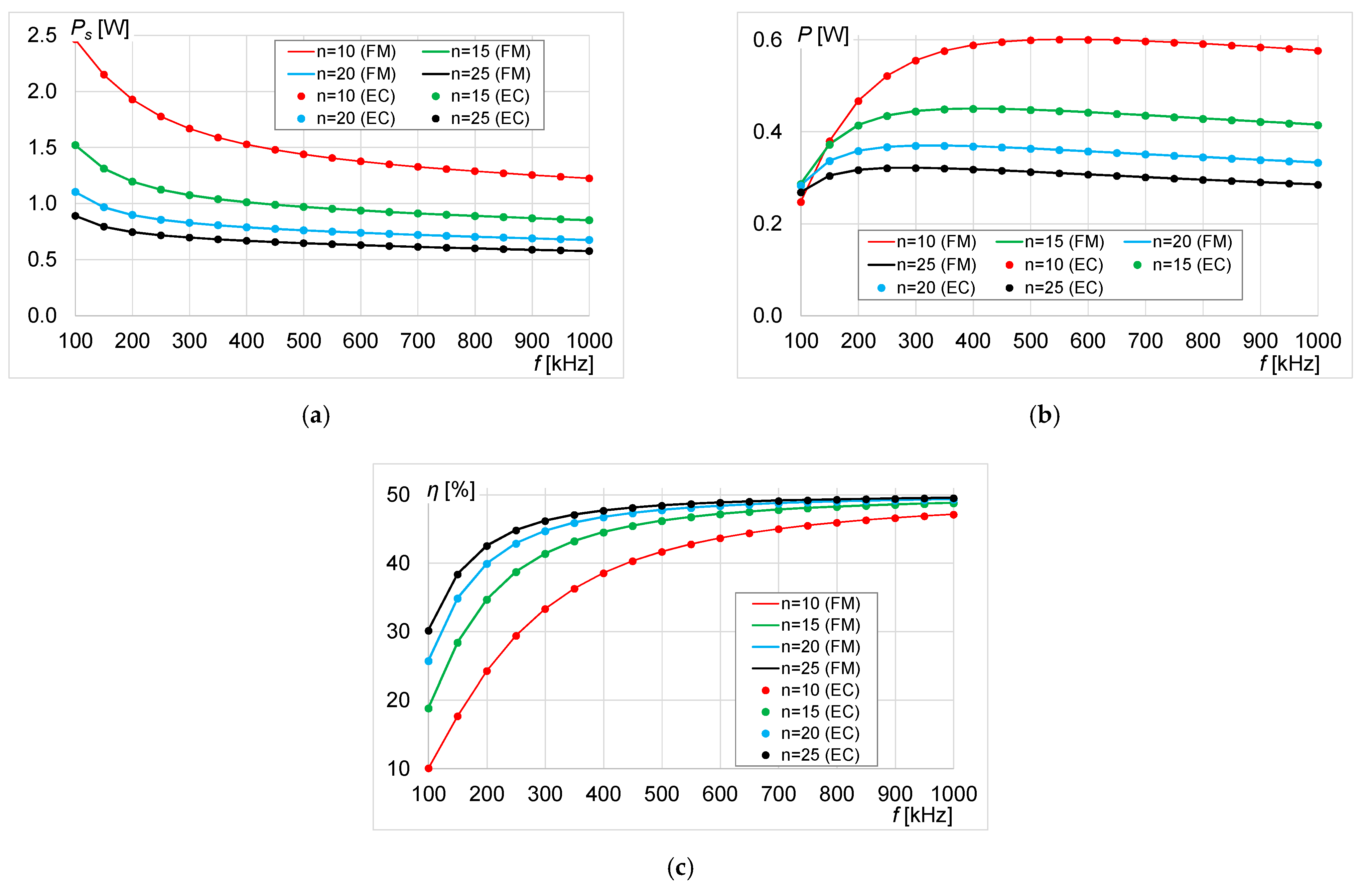
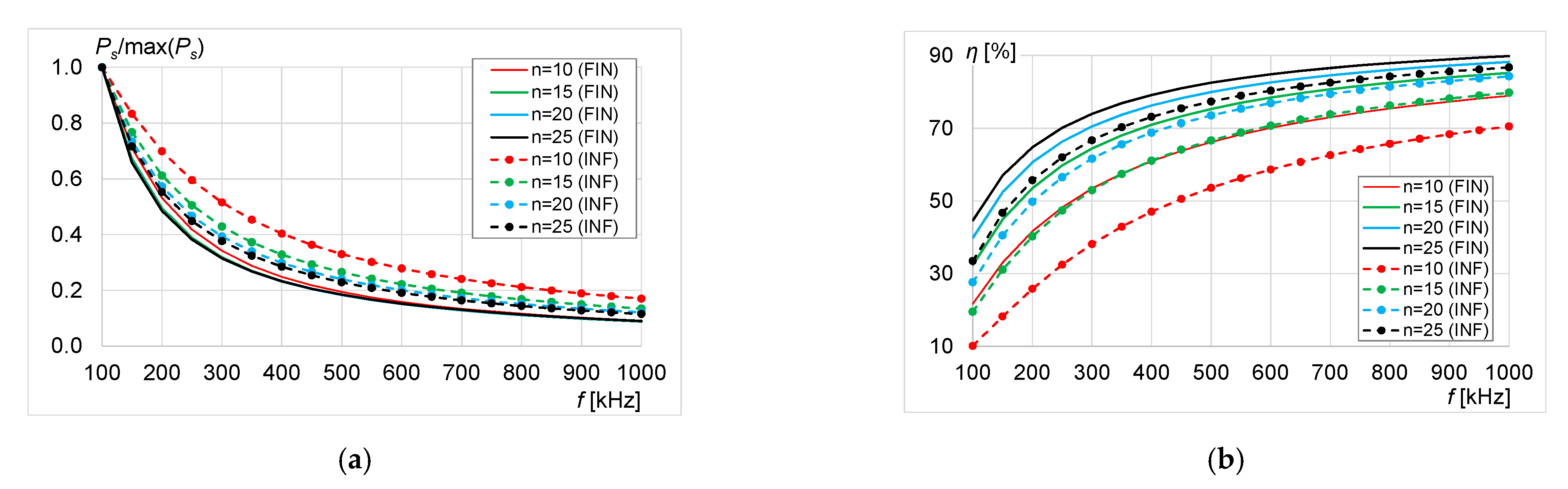
3.2. Analysis of the Infinite Grid

The following results were labeled on characteristics as FM for 3D numerical model (marked with a line) and EC for electrical circuit (marked with a dot). To determine the maximum efficiency, the impedances were calculated for different number of turns, distance between the coils, mutual inductance M_tr and presented in Figure 5. By doubling the distance h the impedance Z_e decreased four times. Still, regardless of the distance between coils, the shape of characteristics remained identical.

Figure 6 and Figure 7 show the characteristics of the source power, load power and efficiency of the system at the distance h = 5 mm between the coils. On all characteristics it can be noted that when the efficiency reaches approximately 50%, the receiver power reaches its maximum value. Then, the receiver power decreases as efficiency exceeded 50%. Despite the nonlinear frequency dependency of powers and efficiency, also the number of turns has a significant impact. By increasing the number of turns the efficiency will rise. Still, only for n = 25 the efficiency of the system had reached the value of nearly 90% at 1 MHz.

In case of larger number of turns (30 ÷ 45) the maximum load power appeared at approximately 100 kHz and then was dropping with rising efficiency (Figure 7). In these cases (h = 5 mm, n = 30 ÷ 45) the number of turns had minor impact on power and efficiency, which reached ≈89% at 1 MHz (Figure 7c). From Figure 7b,c an optimum case for n = 30 can be found, where the highest receiver power was obtained and η was almost as high as for n = 35 ÷ 45. Moreover, comparing the values from numerical model (FM) and equivalent circuit (EC) one may find, that almost perfect agreement have appeared. While FM was a 3D representation of physical system with additional boundary conditions, the EC resulted to be an accurate simplification of the field phenomena.

Figure 8 and Figure 9 show the characteristics for a distance h = 10 mm. Similarly to the case with shorter distance relations between power/efficiency and frequency/number of turns remained almost the same. It was observed that the maximum receiver power values were shifted from 100 kHz to 450 ÷ 750 kHz. Despite the larger distance (h = 10 mm) maximum possible load power was nearly the same as for h = 5 mm and reached approx. 0.2 W. For n = 30 the efficiency was only 3% lower than for n = 35 ÷ 45. In case of a larger number of turns (Figure 9), the efficiency had comparable values at different frequencies, especially for the number of turns n = 35 ÷ 45. Regardless of the number of turns, doubling the distance between the coils caused the efficiency to decrease by ≈30%.

The second operating mode was related with the maximum load power. In order to determine the maximum power transferred to a receiver, the values of load impedance were calculated taking into account the number of turns and distance between coils (Figure 10). An increase in the number of turns causes nonlinear increase of the impedance. While doubling the distance h causes a seventeen times decrease of the impedance but the shape of characteristics was identical.

Figure 11, Figure 12, Figure 13 and Figure 14 show the characteristics of: power (transmitter and receiver) and efficiency at the distance h = 5 mm and h = 10 mm between coils. At considered operation mode (maximum load power) the efficiency of the system tended to max. 50%. For n = 30 ÷ 45 the maximum power is twice as low as for n = 10 ÷ 25. At h = 10 mm the efficiency reaches 50% at above 600 kHz. The exception was the smallest number of turns (n = 10), where maximum efficiency was reached above 1 MHz (Figure 11c).

For h = 5 mm the characteristics of power and efficiency began to stabilize after exceeding a certain frequency. Hence, it was shown the possibility to preserve constant, maximum load power within some frequency range. However, the separation between transmitter and receiver had a crucial impact on this property. At distance h = 10 mm it was noticed that the maximum receiver power, for n = 10 ÷ 25, began to stabilize at frequency at least equal to 1 MHz (Figure 13). Due to the fact that characteristics of power were “stabilizing” along with the efficiency tending to 50%, by increasing n it was possible to compensate this effect and broaden the frequency range of maximum load power (Figure 14). On the other hand, the values of receiver power were smaller than the case n = 10 ÷ 25.

In Figure 15 values of mutual inductance M_tr (between transmitter and receiver) for distances h = 5 mm and h = 10 mm and different number of turns were presented. From n = 10 to n = 35 nearly linear dependency for both distances was observed, where with an increase of the number of turns the mutual inductance increases, too. Nevertheless, doubling the distance between the coils caused a four-fold decrease of mutual inductance.

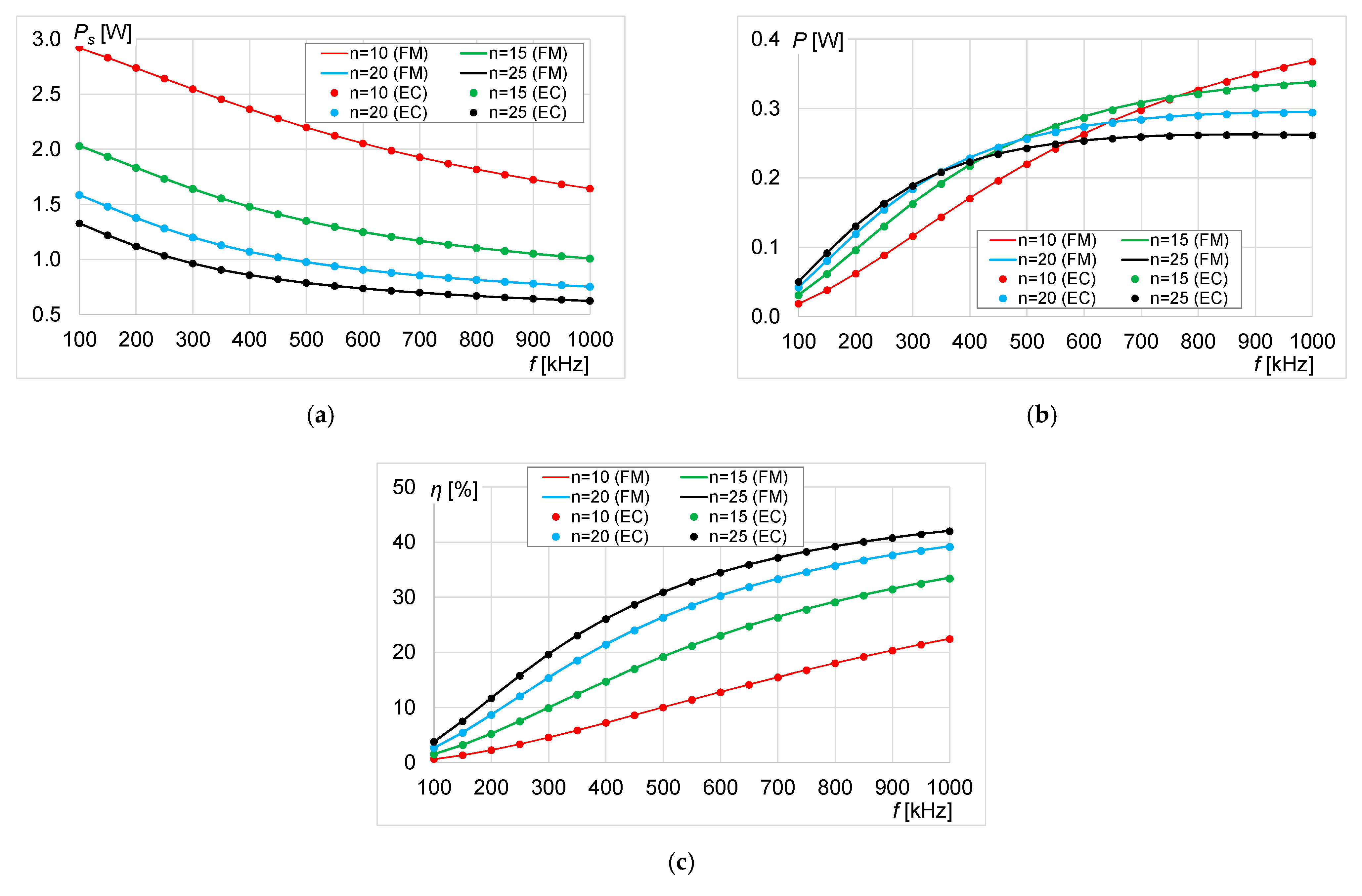
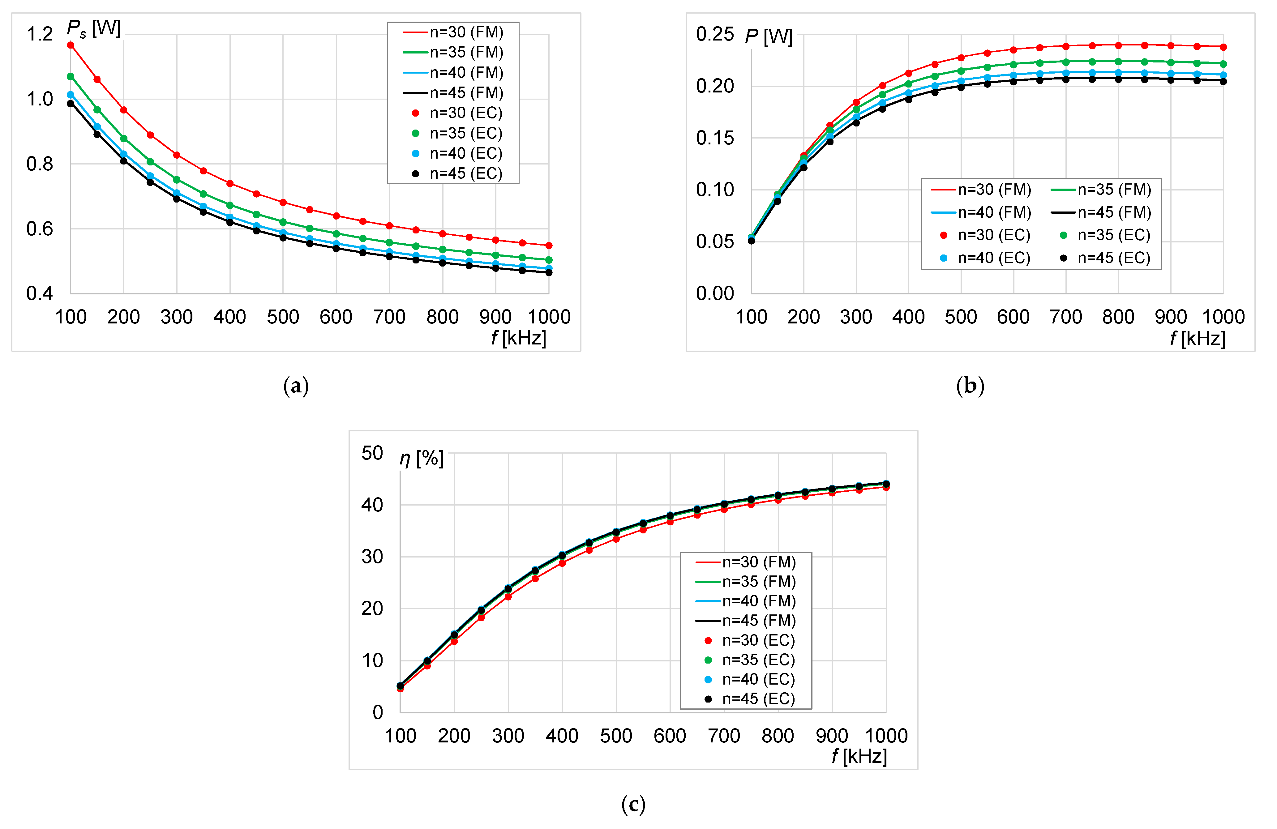
3.3. Analysis of the Finite Grid

An exemplary finite grid of coils was compared with infinite one. Since in grids with small number of resonators the coils on edges and vertices will play dominant role, the approximation with infinite grid is not valid. The most contrasting example is grid of 9 coils with eight coils located at edges (Figure 16). Each coil in grid has mutual inductances:

• with the edge adjacent coils M_edge and with vertex adjacent coils M_vertex;
• with the coil directly above M_tr,vertical, with coils on a side M_tr,side and with coils located diagonally M_tr,diag.

The mutual inductances were gathered in

Table 2. Mutual inductances in a considered grid of nine coils.

n	Mtr,vertical (μH)		Mtr,side (μH)		Mtr,diag (μH)		Medge (μH)	Mvertex (μH)
	h = 0.5 r	h = r	h = 0.5 r	h = r	h = 0.5 r	h = r
10	0.888	0.375	0.053	0.011	0.052	0.011	0.094	0.093
15	1.750	0.721	0.095	0.022	0.093	0.022	0.161	0.159
20	2.662	1.080	0.133	0.034	0.131	0.033	0.218	0.215
25	3.500	1.400	0.164	0.044	0.161	0.043	0.262	0.258
30	4.200	1.647	0.186	0.052	0.183	0.051	0.293	0.289
35	4.680	1.810	0.199	0.057	0.195	0.056	0.311	0.306
40	4.930	1.890	0.205	0.059	0.202	0.058	0.319	0.315
45	5.020	1.930	0.207	0.060	0.204	0.059	0.322	0.318

. For the coil located at the:

• center—there are 4 M_edge with edge adjacent coils and 4 M_vertex couplings with vertex adjacent as well as 1 M_tr,vertical, 4 M_tr,side and 4 M_tr,diag couplings;
• edge—there are 3 M_edge with edge adjacent coils and 2 M_vertex couplings with vertex adjacent as well as 1 M_tr,vertical, 3 M_tr,side and 2 M_tr,diag couplings;
• vertex—there are 2 M_edge with edge adjacent coils and 1 M_vertex coupling with vertex adjacent as well as 1 M_tr,vertical, 2 M_tr,side and 1 M_tr,diag coupling.

The geometrical parameters of coils, and resulting self-impedance, are identical as in Section 3.1. Each transmitting coil was connected with a voltage source (U = 1 V). Moreover, the impedances Z_e were the same as in infinite grid, to preserve identical loads in both compared models. Nonetheless, based on the identified mutual inductances the new values of capacitances were calculated using Equation (11). Then, by solving Equation (18) the currents were found, and then a total load (P) and total source powers (P_s) and the power transfer efficiency (η), using Equation (21), were calculated:

$$P={\displaystyle \sum _{k=1}^{9}Z{\left|{\underset{\_}{I}}_{r,k}\right|}^2}$$

(24)

$$P_s={\displaystyle \sum _{k=1}^{9}U\left|{\underset{\_}{I}}_{t,k}\right|}$$

(25)

The results presented in Figure 17, Figure 18, Figure 19 and Figure 20 were labeled as FIN for the finite grid and INF for infinite grid. The shape of characteristics remained similar for both types of WPT systems, but values of the relative source power and power transfer efficiency were different. The total source power was always lower in finite grid, while the efficiency was higher. This can be easily explained, since in finite grid occurred the lesser amount of mutual inductances, which were negatively affecting mutual inductance between transmitter and receiver (higher L_c due to lower M_period).

At the distance h = r/2 = 5 mm these differences were mostly noticeable for n = 10 (Figure 17b). For example, the efficiency was about 12% lower in the infinite grid. With higher number of turns the differences were smaller, e.g., for n = 25 the efficiency was only 6% lower. For considered number of turns n = 30 ÷ 45, both shapes and values of the characteristics were similar (Figure 18). The divergences between relative source power in finite and infinite grid were within acceptable range. However, efficiency was higher in the finite grid (average difference between FIN and INF equal to 4.58%).

At the distance h = r = 10 mm the source power calculated in the infinite grid was several times higher than in finite network of resonators, which was observed for each number of turns (Figure 19a and Figure 20a). The power transfer efficiency was directly related with source and load powers, hence visible differences had also occurred. For example, at f = 1 MHz and n = 10 the efficiency of power transfer in finite grid was 53.2% while in infinite 23.6%. Once more for n = 30 ÷ 45 these divergences were smaller, but still significant (at f = 1 MHz and n = 45 the efficiency in finite grid was 75.2% and in infinite 59.7%).

4. Conclusions

The maximum efficiency and load power in periodic WPT systems were estimated based on exemplary structures with many magnetic couplings between constituent inductors. The models used for an analysis of considered structures, arranged of many spiral planar coils, were developed. In the article, two types of simulated models were used: a 3D numerical representation of the system solved by finite element method and the equivalent circuits with lumped parameters. The purpose was to quickly determine the output parameters (e.g., power, efficiency) both with 3D numerical model and by using its equivalent circuit. The utilization of electrical circuit, representing a single cell of the WPT system, eliminated the need to make very complex numerical models. Nevertheless, the article presented the structure of the 3D model and conditions that help to reduce its complexity. The next step of further investigation will be focused on conducting experimental verification of the theoretical results to assess a suitability of the proposed models.

The given solutions, adopted in the numerical and electrical models, allow studying the influence of the coil geometry and a distance between transmitter and receiver on the power transmission. Calculations were performed over a wide frequency range. The analysis concerned the influence of geometrical parameters of coils in the WPT cell (e.g., number of turns) on the efficiency of system and the power of transmitter and receiver. By simply adjusting the number of turns and increasing frequency of a current, it was possible to obtain high efficiency of power transmission (≈90%) for the loads supplied using proposed system, without the use of intermediate coils or iron cores/bars. Even at distances equal to a radius of coil the system was still able to reach near 60% efficiency.

Additionally, the results of obtaining maximum load power were presented. By appropriate selection of load impedance it was possible to determine the power transferred to receiver and a corresponding efficiency. Similarly to the previous case, the results from proposed equivalent circuit were consistent with results from the 3D numerical model. The negligible differences in results confirmed a correctness of the adopted assumptions and shown, that the analysis of an extensive grid of periodic resonators can be simplified to a single WPT cell, modeled as two-port circuit with lumped parameters.

Finally, the finite WPT grid of resonators was compared with the infinite network of resonators. While the source power and efficiency had almost identical frequency dependence, the values were noticeably different. This was due to the fact that finite grid of only several magnetically coupled resonators was characterized by the lesser amount of mutual inductances, which negatively affected wireless power transfer between transmitter and receiver coil. Considered examples had shown that infinite approximation of periodic WPT system was valid only for very large grids with many resonators. For small grids edge effects, related with coils located at edges and vertexes of a surface, had to be taken into account to accurately calculate the power of source, load and the efficiency.

References

1. Barman, S.D.; Reza, A.W.N.; Kumar, N.; Karim, M.E.; Munir, A.B. Wireless powering by magnetic resonant coupling: Recent trends in wireless power transfer system and its applications. Renew. Sustain. Energy Rev. 2015, 51, 1525–1552. [Google Scholar] [CrossRef]
2. Kuo, R.-C.; Riehl, P.; Satyamoorthy, A.; Plumb, W.; Tustin, P.; Lin, J. A 3D resonant wireless charger for a wearable device and a mobile phone. In Proceedings of the 2015 IEEE Wireless Power Transfer Conference (WPTC), Boulder, CO, USA, 13–15 May 2015. [Google Scholar]
3. Zable, M.A.H.; Khan, Z.I.; Zakaria, N.A.; Abd Rashid, N.E.; Shariff, K.K.M.; Enche Ab Rahim, S.A. Performance Evaluation of WPT Circuit suitable for Wireless Charging. In Proceedings of the 2020 IEEE Symposium on Industrial Electronics & Applications (ISIEA), TBD, Malaysia, 17–18 July 2020. [Google Scholar]
4. Sun, L.; Ma, D.; Tang, H. A review of recent trends in wireless power transfer technology and its applications in electric vehicle wireless charging. Renew. Sustain. Energy Rev. 2018, 91, 490–503. [Google Scholar] [CrossRef]
5. Luo, Z.; Wei, X. Analysis of Square and Circular Planar Spiral Coils in Wireless Power Transfer System for Electric Vehicles. IEEE Trans. Ind. Electron. 2018, 65, 331–341. [Google Scholar] [CrossRef]
6. Batra, T.; Schaltz, E.; Ahn, S. Effect of ferrite addition above the base ferrite on the coupling factor of wireless power transfer for vehicle applications. J. Appl. Phys. 2015, 117, 17D517. [Google Scholar] [CrossRef]
7. Eteng, A.A.; Rahim, S.K.A.; Leow, C.Y.; Chew, B.W.; Vandenbosch, G.A.E. Two-Stage Design Method for Enhanced Inductive Energy Transmission with Q-Constrained Planar Square Loops. PLoS ONE 2016, 11, e0148808. [Google Scholar] [CrossRef] [Green Version]
8. Kim, T.-H.; Yun, G.-H.; Lee, W.Y. Asymmetric Coil Structures for Highly Efficient Wireless Power Transfer Systems. IEEE Trans. Microw. Theory Tech. 2018, 66, 3443–3451. [Google Scholar] [CrossRef]
9. Rim, C.T.; Mi, C. Wireless Power Transfer for Electric Vehicles and Mobile Devices; John Wiley & Sons, Ltd.: Hoboken, NJ, USA, 2017; pp. 473–490. [Google Scholar]
10. Fujimoto, K.; Itoh, K. Antennas for Small Mobile Terminals, 2nd ed.; Artech House: Norwood, MA, USA, 2018; pp. 30–70. [Google Scholar]
11. Zhang, Z.; Pang, H.; Georgiadis, A.; Cecati, C. Wireless Power Transfer—An Overview. IEEE Trans. Ind. Electron. 2019, 66, 1044–1058. [Google Scholar] [CrossRef]
12. Rozman, M.; Fernando, M.; Adebisi, B.; Rabie, K.M.; Collins, T.; Kharel, R.; Ikpehai, A. A New Technique for Reducing Size of a WPT System Using Two-Loop Strongly-Resonant Inductors. Energies 2017, 10, 1614. [Google Scholar] [CrossRef] [Green Version]
13. Liu, X.; Wang, G. A Novel Wireless Power Transfer System with Double Intermediate Resonant Coils. IEEE Trans. Ind. Electron. 2016, 63, 2174–2180. [Google Scholar] [CrossRef]
14. El Rayes, M.M.; Nagib, G.; Abdelaal, W.G.A. A Review on Wireless Power Transfer. IJETT 2016, 40, 272–280. [Google Scholar] [CrossRef]
15. Re, P.D.H.; Podilchak, S.K.; Rotenberg, S.; Goussetis, G.; Lee, J. Circularly Polarized Retrodirective Antenna Array for Wireless Power Transmission. In Proceedings of the 2017 11th European Conference on Antennas and Propagation (EUCAP), Paris, France, 19–24 March 2017; pp. 891–895. [Google Scholar]
16. Nikoletseas, S.; Yang, Y.; Georgiadis, A. Wireless Power Transfer Algorithms, Technologies and Applications in Ad Hoc Communication Networks; Springer: Cham, Switzerland, 2016; pp. 31–51. [Google Scholar]
17. Stevens, C.J. Magnetoinductive waves and wireless power transfer. IEEE Trans. Power Electron. 2015, 30, 6182–6190. [Google Scholar] [CrossRef]
18. Zhong, W.; Lee, C.K.; Hui, S.Y.R. General analysis on the use of Tesla’s resonators in domino forms for wireless power transfer. IEEE Trans. Ind. Electron. 2013, 60, 261–270. [Google Scholar] [CrossRef] [Green Version]
19. Alberto, J.; Reggiani, U.; Sandrolini, L.; Albuquerque, H. Accurate calculation of the power transfer and efficiency in resonator arrays for inductive power transfer. PIER 2019, 83, 61–76. [Google Scholar] [CrossRef] [Green Version]
20. Alberto, J.; Reggiani, U.; Sandrolini, L.; Albuquerque, H. Fast calculation and analysis of the equivalent impedance of a wireless power transfer system using an array of magnetically coupled resonators. Prog. Electromagn. Res. 2018, 80, 101–112. [Google Scholar] [CrossRef] [Green Version]
21. Martin, P.; Ho, B.J.; Grupen, N.; Muñoz, S.; Srivastasa, M. An iBeacon Primer for Indoor Localization. In Proceedings of the 1st ACM Conference on Embedded Systems for Energy-Efficient Buildings (BuildSys’14), Memphis, TN, USA, 3–6 November 2014; pp. 190–191. [Google Scholar]
22. Li, X.; Zhang, H.; Peng, F.; Li, Y.; Yang, T.; Wang, B.; Fang, D. A wireless magnetic resonance energy transfer system for micro implantable medical sensors. Sensors 2012, 12, 10292–10308. [Google Scholar] [CrossRef] [PubMed]
23. Fitzpatrick, D.C. Implantable Electronic Medical Devices; Academic Press: San Diego, CA, USA, 2014; pp. 7–35. [Google Scholar]
24. Kim, D.; Abu-Siada, A.; Sutinjo, A. State-of-the-art literature review of WPT: Current limitations and solutions on IPT. Electric Power Syst. Res. 2018, 154, 493–502. [Google Scholar] [CrossRef]
25. Kesler, M. Highly Resonant Wireless Power Transfer: Safe, Efficient and Over Distance; WiTricity Corporation: Watertown, MA, USA, 2013. [Google Scholar]
26. Tal, N.; Morag, Y.; Levron, Y. Magnetic Induction Antenna Arrays for MIMO and Multiple-Frequency Communication Systems. Prog. Electromagn. Res. 2017, 75, 155–167. [Google Scholar] [CrossRef] [Green Version]
27. IEC 60364-7. Requirements for Special Installations or Locations; IEC: Geneva, Switzerland, 2017. [Google Scholar]
28. Mohan, S.S.; del Mar Hershenson, M.; Boyd, S.P.; Lee, T.H. Simple Accurate Expressions for Planar Spiral Inductances. IEEE J. Solid-State Circuits 1999, 34, 1419–1424. [Google Scholar] [CrossRef] [Green Version]
29. Liu, S.; Su, J.; Lai, J. Accurate Expressions of Mutual Inductance and Their Calculation of Archimedean Spiral Coils. Energies 2019, 12, 2017. [Google Scholar] [CrossRef] [Green Version]
30. Knight, D.W. Practical continuous functions for the internal impedance of solid cylindrical conductors. G3YNH 2016. [Google Scholar] [CrossRef]
31. Li, Y.; Song, K.; Li, Z.; Jiang, J.; Zhu, C. Optimal Efficiency Tracking Control Scheme Based on Power Stabilization for a Wireless Power Transfer System with Multiple Receivers. Energies 2018, 11, 1232. [Google Scholar] [CrossRef] [Green Version]
Figure 1. Configurations of periodic wireless power transfer systems: (a) the geometry of a proposed periodic WPT structure and (b) an application of WPT cells as a separated extra-low voltage energy supply system for LED lightning in dangerous areas.
Energies 14 01151 g001
Figure 2. A fragment of the transmitting/receiving surface of the periodic WPT system.
Energies 14 01151 g002
Figure 3. (a) The spiral coil made of several turns (n) of a wire with a diameter (w) and an insulation thickness (s) and (b) the three-dimensional model of a single WPT cell.
Energies 14 01151 g003
Figure 4. Circuit models of periodic WPT system: (a) topology and magnetic couplings in a resonator grid from the point of view of an arbitrary coil Ax, y and (b) simplified equivalent circuit model of a WPT cell Ax, y in an infinite grid.
Energies 14 01151 g004
Figure 5. Optimum load impedance at fmax to obtain the maximum efficiency at distances: (a) h = 5 mm and (b) h = 10 mm.
Energies 14 01151 g005
Figure 6. Results at the distance h = 5 mm and number of turns n = 10 ÷ 25: (a) transmitter power, (b) receiver power and (c) power transfer efficiency.
Energies 14 01151 g006
Figure 7. Results at the distance h = 5 mm and number of turns n = 30 ÷ 45: (a) transmitter power, (b) receiver power and (c) power transfer efficiency.
Energies 14 01151 g007
Figure 8. Results at the distance h = 10 mm and number of turns n = 10 ÷ 25: (a) transmitter power, (b) receiver power and (c) power transfer efficiency.
Energies 14 01151 g008
Figure 9. Results at the distance h = 10 mm and number of turns n = 30 ÷ 45: (a) transmitter power, (b) receiver power and (c) power transfer efficiency.
Energies 14 01151 g009
Figure 10. Optimum load impedance at fmax to obtain the maximum load power at distances: (a) h = 5 mm and (b) h = 10 mm.
Energies 14 01151 g010
Figure 11. Results at the distance h = 5 mm and number of turns n = 10 ÷ 25: (a) transmitter power, (b) receiver power and (c) power transfer efficiency.
Energies 14 01151 g011
Figure 12. Results at the distance h = 5 mm and number of turns n = 30 ÷ 45: (a) transmitter power, (b) receiver power and (c) power transfer efficiency.
Energies 14 01151 g012
Figure 13. Results at the distance h = 10 mm and number of turns n = 10 ÷ 25: (a) transmitter power, (b) receiver power and (c) power transfer efficiency.
Energies 14 01151 g013
Figure 14. Results at the distance h = 10 mm and number of turns n = 30 ÷ 45: (a) transmitter power, (b) receiver power and (c) power transfer efficiency.
Energies 14 01151 g014
Figure 15. Mutual inductance Mtr between transmitter and receiver at distances: (a) h = 5 mm and (b) h = 10 mm.
Energies 14 01151 g015
Figure 16. An arrangement of coils in a finite periodic grid of WPT cells with mutual inductances in horizontal and vertical planes.
Energies 14 01151 g016
Figure 17. Results at the distance h = 5 mm and number of turns n = 10 ÷ 25: (a) total source power and (b) efficiency.
Energies 14 01151 g017
Figure 18. Results at the distance h = 5 mm and number of turns n = 30 ÷ 45: (a) total source power and (b) efficiency.
Energies 14 01151 g018
Figure 19. Results at the distance h = 10 mm and number of turns n = 10 ÷ 25: (a) total source power and (b) efficiency.
Energies 14 01151 g019
Figure 20. Results at the distance h = 10 mm and number of turns n = 30 ÷ 45: (a) total source power and (b) efficiency.
Energies 14 01151 g020