
Simulation-Based Optimization of Microbial Enhanced Oil Recovery with a Model Integrating Temperature, Pressure, and Salinity Effects


Abstract
1. Introduction
2. Methods
2.1. Fluid Flow in Permeable Media
2.2. Stoichiometric Equations
2.3. Microbial Reaction Rate
2.4. Environmental Factor Effects on Reaction Rate
2.4.1. Temperature
2.4.2. Pressure
2.4.3. Salinity
2.5. Permeability Reduction Model
2.6. History Matching Error
2.7. Proxy Model for Sensitivity Analysis and Optimization
3. Results
3.1. Batch and Sandpack Model Simulation
3.2. Verification of Models Reflecting Environmental Factors
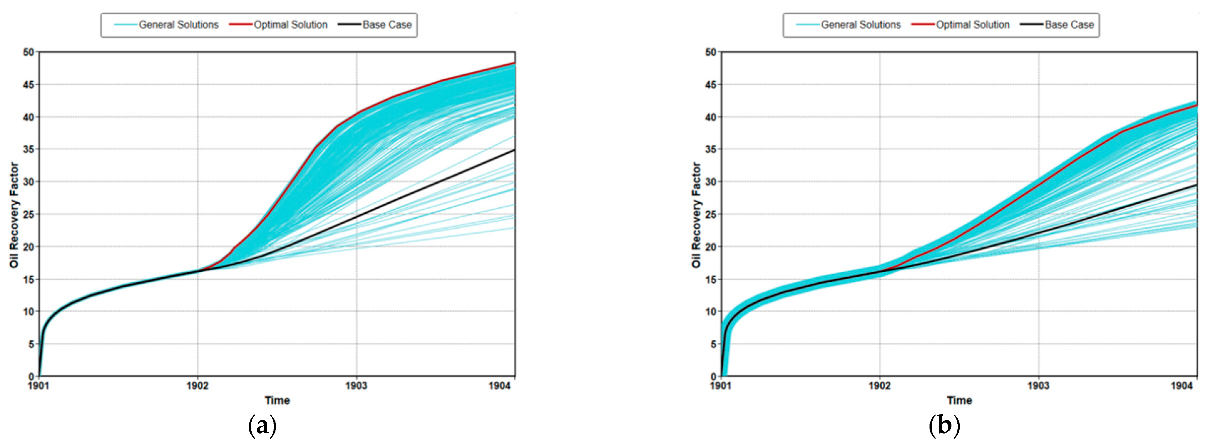
3.3. Optimization of MEOR
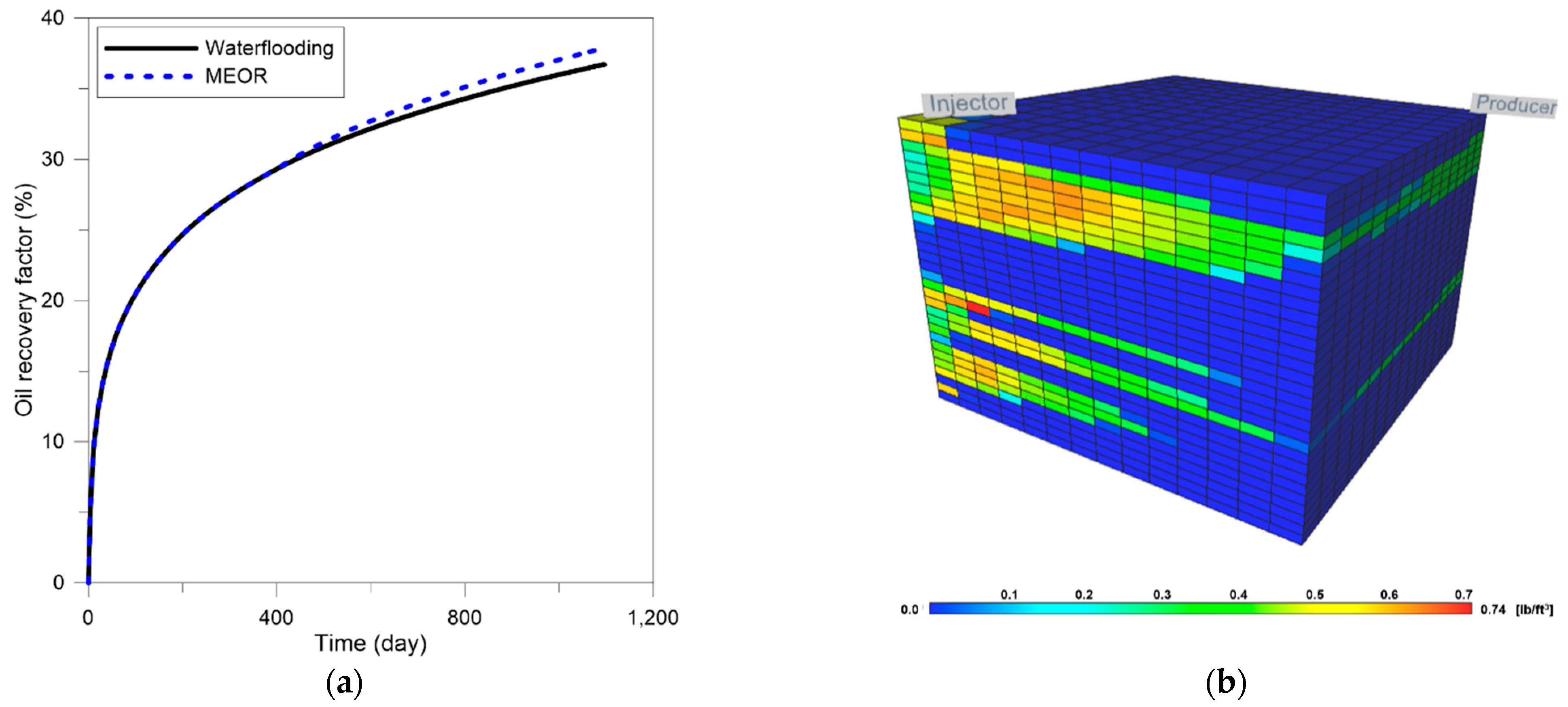
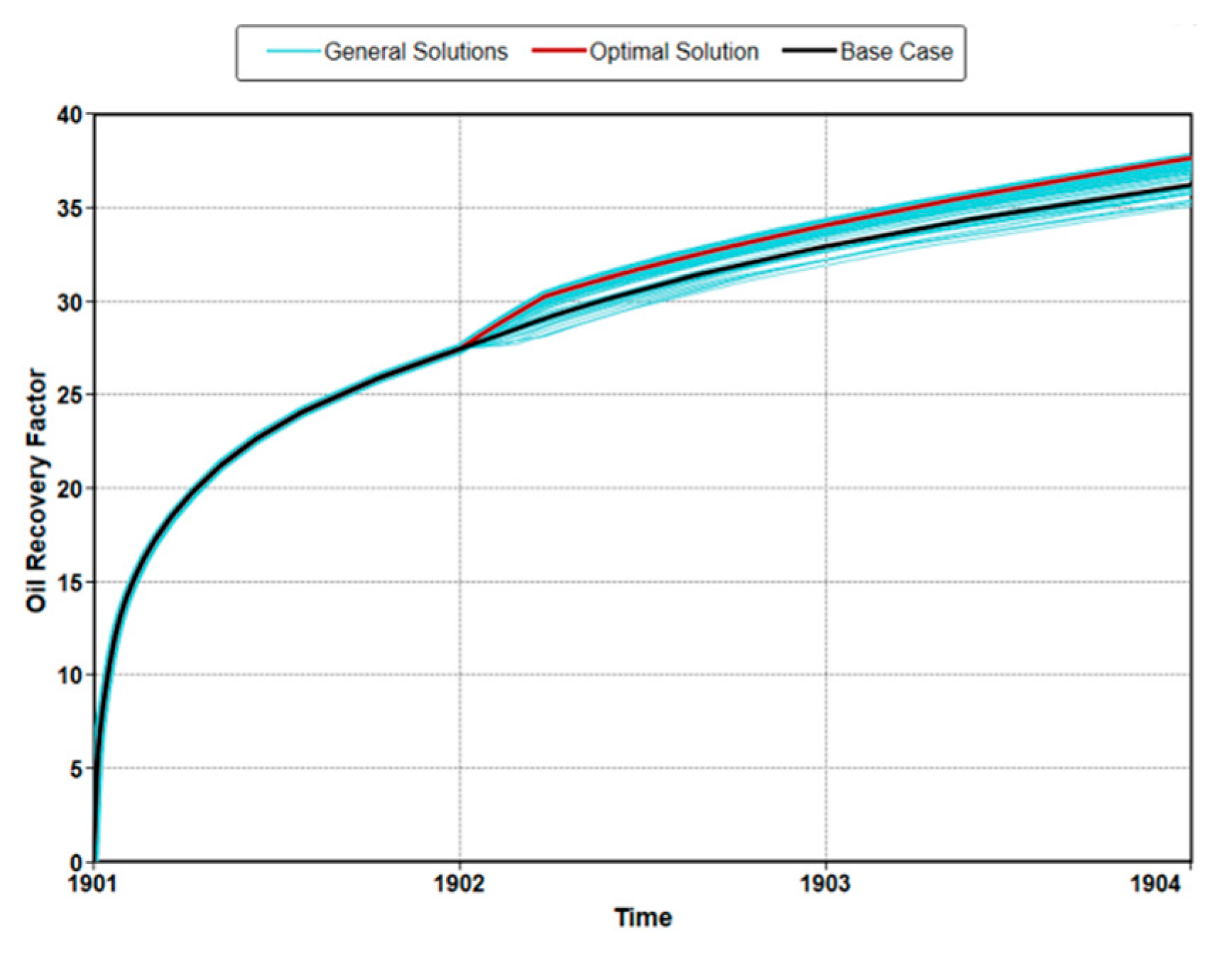
3.4. Field Application
4. Conclusions
Author Contributions
Funding
Institutional Review Board Statement
Informed Consent Statement
Conflicts of Interest
Nomenclature
| A | constant | a0 | intercept |
| aij | coefficients of interaction terms | Aj | constant of the j-th step |
| aj | coefficients of linear terms | ajj | coefficients of quadratic terms |
| B | constant | ci | concentration of component i |
| cNaCl | NaCl concentration | upper limit of NaCl concentration for microbial growth | |
| optimum NaCl concentration for microbial growth | cs | concentration of the solid phase | |
| csucrose | sucrose concentration | D | decimal reduction time |
| Dj | decimal time of the j-th step | Dji | component dispersibility (j = w, o, g) |
| E | history matching error | Ea | activation energy |
| Ea,j | activation energy of the j-th step | Fdiv | division factor |
| FFreq | frequency factor | FFreq,p | frequency factor for each pressure step |
| K | transmissibility | dispersion tensor | |
| k | changed permeability | k50 | mean permeability at 50% probability |
| k81.4 | permeability at 84.1% probability | kmul | multiplier factor |
| ko | initial permeability | N | number of surviving microbes |
| n | constant | NC | number of components (or ) |
| nf | number of neighboring regions or grid block faces | No | initial number of microbes |
| NP | number of phases | Merr | measurement error |
| mi | mass fraction of component i | pj | pressure of the j-th step |
| qik | phase rates in layer k (j = w, o, g) | R | gas constant |
| r | kinetic reaction rate | rdecay | reaction rate for bacterial decay |
| rdecay, p | reaction rate as affected by pressure | rNaCl | reaction rate as a function of NaCl |
| rNaCl,backward | backward reaction rate by NaCl | ropt | optimum reaction rate |
| rtemp | reaction rate as a function of temperature | S | saturation |
| s | normalization scale | T | temperature |
| t | time | telap | elapsed time |
| tp | pressure-hold time | Tj | temperature of the j-th step |
| Tmax | upper limit for growth temperature | Tmin | lower limit for growth temperature |
| Topt | optimum temperature for microbial growth | superficial velocity | |
| VDP | Dykstra–Parsons coefficient | Vf | volume of fluid phase |
| wi | mole fraction of component i in aqueous phase | xi | mole fraction of component i in oil phase |
| xixj | interaction effects of parameters | xj | linear effect of parameters |
| quadratic effects of the parameters | y | objective function | |
| yi | mole fraction of component i in gas phase | ΔΥm | measured maximum change |
| measured result | simulated result | ||
| zp | negative reciprocal slope of log D vs. p | ||
| Subscript | |||
| g | gas phase | k | layer k |
| o | oil phase | s | solid phase |
| w | water phase | ||
| Greek | |||
| α | rate constant | ρ | density |
| Φ | potential | ɸ | porosity |
| ɸo | initial porosity | ||
Appendix A

 | Growth Media Composition (Mole Fraction) | |
| Sucrose | 0.000789 | |
| NH4+ | 0.000133 | |
| HCO3− | 0.000219 | |
| H2O | 0.99883 | |
| Microbes | 2.92 × 10⁻⁵ | |
 | Model Conditions | |
| Size (mm3) | 62.1 × 62.1 × 160 | |
| Initial Porosity | 0.38 | |
| Initial Permeability (md) | 4150 | |
| Injector Location | 1, 1, 20 (bottom block) | |
| Producer Location | 1, 1, 1 (top block) | |
| Pressure Measurement | (1, 1, 8) and (1, 1, 13) | |
| Permeability Distribution | ||
|---|---|---|
 | ||
| Initial Conditions | ||
| Size (ft3) | 200 × 10 × 100 | |
| Grid | 20 × 1 × 10 | |
| Temperature (°F) | 100 | |
| Pressure (psi) | 4000 | |
| NaCl concentration (%) | 10 | |
| Permeability (md) | High-k zone | 1000 |
| Low-k zone | 50 | |
| Porosity | 0.25 | |
| Saturation | Oil | 0.8 |
| Water | 0.2 | |
| Relative Permeability: Brooks–Corey Model | ||
| Connate water saturation | 0.3 | |
| Irreducible oil saturation | 0.2 | |
| krw at irreducible oil | 0.5 | |
| kro at connate water | 0.8 | |
| Exponent for krw | 2 | |
| Exponent for kro | 2 | |
Appendix B
References
- Davarpanah, A. A feasible visual investigation for associative foam>/ polymer injectivity performances in the oil recovery enhancement. Eur. Polym. J. 2018, 105, 405–411. [Google Scholar] [CrossRef]
- Davarpanah, A.; Mirshekari, B. Experimental investigation and mathematical modeling of gas diffusivity by carbon dioxide and methane kinetic adsorption. Ind. Eng. Chem. Res. 2019, 58, 12392–12400. [Google Scholar] [CrossRef]
- Davarpanah, A.; Mirshekari, B. Numerical simulation and laboratory evaluation of alkali-surfactant-polymer and foam flooding. Int. J. Environ. Sci. Technol. 2019, 17, 1123–1136. [Google Scholar] [CrossRef]
- Davarpanah, A. Parametric study of polymer-nanoparticles-assisted injectivity performance for axisymmetric two-phase flow in EOR processes. Nanomaterials 2020, 10, 1818. [Google Scholar] [CrossRef] [PubMed]
- Hu, X.; Xie, J.; Cai, W.; Wang, R.; Davarpanah, A. Thermodynamic effects of cycling carbon dioxide injectivity in shale reservoirs. J. Pet. Sci. Eng. 2020, 195, 107717. [Google Scholar] [CrossRef]
- Pan, F.; Xhang, Z.; Zhang, X.; Davarpanah, A. Impact of anionic and cationic surfactants interfacial tension on the oil recovery enhancement. Powder Technol. 2020, 373, 93–98. [Google Scholar] [CrossRef]
- Hu, Y.; Cheng, Q.; Yang, J.; Zhang, L.; Davarpanah, A. A laboratory approach on the hybrid-enhanced oil recovery techniques with different saline brines in sandstone reservoirs. Processes 2020, 8, 1051. [Google Scholar] [CrossRef]
- Belyaev, S.S.; Borzenkov, I.A.; Nazina, T.N.; Rozanova, E.P.; Glumov, I.F.; Ibatullin, R.R.; Ivanov, M.V. Use of microorganisms in the biotechnology for the enhancement of oil recovery. Microbiology 2004, 73, 590–598. [Google Scholar] [CrossRef]
- Lazar, I.; Petrisor, I.G.; Yen, T.F. Microbial enhanced oil recovery (MEOR). Pet. Sci. Technol. 2007, 25, 1353–1366. [Google Scholar] [CrossRef]
- Guo, H.; Li, Y.; Yiran, Z.; Wang, F.; Wang, Y.; Yu, Z.; Haicheng, S.; Yuanyuan, G.; Chuyi, J.; Xian, G. Progress of Microbial Enhanced Oil Recovery in China. In Proceedings of the SPE Asia Pacific Enhanced Oil Recovery Conference, Kuala Lumpur, Malaysia, 11–13 August 2015. [Google Scholar]
- Jenneman, G.E.; Moffitt, P.D.; Young, G.R. Application of a microbial selective-plugging process at the North Burbank Unit: Prepilot tests. SPE Prod. Facil. 1996, 11, 11–17. [Google Scholar] [CrossRef]
- Brown, L.R.; Vadie, A.A.; Stephens, J.O. Slowing production decline and extending the economic life of an oil field: New MEOR technology. SPE Reserv. Eval. Eng. 2002, 5, 33–41. [Google Scholar] [CrossRef]
- Cusack, F.M.; Singh, S.; Novosad, J.; Chmilar, M.; Blenknsopp, S.A.; Costerton, J.W. The Use of Ultramicrobacteria for Selective Plugging in Oil Recovery by Waterflooding. In Proceedings of the International Meeting on Petroleum Engineering, Beijing, China, 24–27 March 1992. [Google Scholar]
- Jack, T.R.; Stehmeier, L.G.; Islam, M.R.; Ferris, F.G. Microbial selective plugging to control water channeling. In Microbial Enhancement of Oil Recovery–Recent Advances; Donaldson, E.C., Ed.; Elsevier: Amsterdam, The Netherland, 1991; pp. 433–440. [Google Scholar]
- Hitzman, D.O. Review of Microbial Enhanced Oil Recovery Field Tests. In Proceedings of the Symposium on Applications of Microorganisms to Petroleum Technology, Bartlesville, OK, USA, 12–13 August 1987. [Google Scholar]
- Patel, J.; Borgohain, S.; Kumar, M.; Rangarajan, V.; Somasundaran, P.; Sen, R. Recent developments in microbial enhanced oil recovery. Renew. Sustain. Energy Rev. 2015, 52, 1539–1558. [Google Scholar] [CrossRef]
- Safdel, M.; Anbaz, M.A.; Daryasafar, A.; Jamialahmadi, M. Microbial enhanced oil recovery, a critical review on worldwide implemented field trials in different countries. Renew. Sustain. Energy Rev. 2017, 74, 159–172. [Google Scholar] [CrossRef]
- Wang, J.; Xu, H.; Guo, S. Isolation and characteristics of a microbial consortium for effectively degrading phenanthrene. Pet. Sci. 2007, 4, 68–75. [Google Scholar] [CrossRef]
- Sen, R. Biotechnology in petroleum recovery: The microbial EOR. Prog. Energy Combust. Sci. 2008, 34, 714–724. [Google Scholar] [CrossRef]
- Darvishi, P.; Ayatollahi, S.; Mowla, D.; Niazi, A. Biosurfactant production under extreme environmental conditions by efficient microbial consortium, ERCPPI-2. Colloids Surf. B Biointerfaces 2011, 84, 292–300. [Google Scholar] [CrossRef]
- Stanier, R.Y.; Doudoroff, M.; Adelberg, E.A. The Microbial World, 3rd ed.; Prentice-Hall: Englewood Cliffs, NJ, USA, 1970. [Google Scholar]
- Brock, T.D.; Brock, K.M.; Belly, R.T.; Weiss, R.L. Sulfolobus: A new genus of sulfur-oxidizing bacteria living at low pH and high temperature. Arch. Microbiol. 1972, 84, 54–68. [Google Scholar] [CrossRef] [PubMed]
- Brock, T.D. Thermophilic Microorganisms and Life at High Temperatures; Springer: New York, NY, USA, 1978. [Google Scholar]
- Corliss, J.B.; Dymond, J.; Gordon, L.I.; Edmond, J.M.; von Herzen, R.P.; Ballard, R.D.; Green, K.; Williams, D.; Bainbridge, A.; Crane, K.; et al. Submarine thermal springs on the Galápagos Rift. Science 1979, 203, 1073–1083. [Google Scholar] [CrossRef]
- Karl, D.M.; Wirsen, C.O.; Jannasch, H.W. Deep-sea primary production at the Galápagos hydrothermal vents. Science 1980, 207, 1345–1347. [Google Scholar] [CrossRef]
- Jannash, H.W.; Wirsen, C.O. Morphological survey of microbial mats near deep-sea thermal vents. Appl. Environ. Microbiol. 1981, 41, 528–538. [Google Scholar] [CrossRef]
- Baross, J.A.; Liley, M.D.; Gordon, L.I. Is the CH4, H2 and CO venting from submarine hydrothermal systems produced by thermophilic bacteria? Nature 1982, 298, 366–368. [Google Scholar] [CrossRef]
- Yayanos, A.A.; Dietz, A.S. Thermal inactivation of a deep-sea barophilic bacterium, isolate CNPT-3. Appl. Environ. Microbiol. 1982, 43, 1481–1489. [Google Scholar] [CrossRef]
- Leigh, J.A.; Jones, J.W. A New Extremely Thermophilic Methanogen from a Submarine Hydrothermal Vent. In Proceedings of the 83rd Annual Meeting of the American Society for Microbiology, New Orleans, LA, USA, 6–11 March 1983. [Google Scholar]
- Villadsen, J.; Nielsen, J.; Lidén, G. Bioreaction Engineering Principles; Springer Science and Business Media: Berlin, Germany, 2011. [Google Scholar]
- Zobell, C.E. Pressure effects on morphology and life processes of bacteria. In High Pressure Effects on Cellular Processes; Zimmerman, A.M., Ed.; Academic Press: New York, NY, USA, 1970; pp. 85–130. [Google Scholar]
- Morita, R.Y. Pressure: Bacteria, fungi and blue-green algae. In Marine Ecology; Kinne, Ed.; Wiley: New York, NY, USA, 1972; pp. 1361–1388. [Google Scholar]
- Marquis, R.E.; Matsumura, P. Microbial life under pressure. In Microbial Life in Extreme Environments; Kushner, D.J., Ed.; Academic Press: London, UK, 1978; pp. 105–158. [Google Scholar]
- Marquis, R.E. Barobiology of Deep Oil Formations. In Proceedings of the International Conference on Microbial Enhancement of Oil Recovery, Afton, OK, USA, 16 May 1983. [Google Scholar]
- Basak, S.; Ramaswamy, H.S.; Piette, J.P.G. High pressure destruction kinetics of Leuconostoc mesenteroides and Saccharomyces cerevisiae in single strength and concentrated orange juice. Innov. Food Sci. Emerg. Technol. 2002, 3, 223–231. [Google Scholar] [CrossRef]
- Stanley, S.O.; Morita, R.Y. Salinity effect on the maximal growth temperature of some bacteria isolated from marine environments. J. Bacteriol. 1968, 95, 169–173. [Google Scholar] [CrossRef]
- Bilsky, A.Z.; Armstrong, J.B. Osmotic reversal of temperature sensitivity in Escherichia coli. J. Bacteriol. 1973, 113, 76–81. [Google Scholar] [CrossRef]
- Boyer, E.W.; Ingle, M.B.; Mercer, G.D. Bacillus alcalophilus subsp. halodurans subsp. nov.: An alkaline-amylase-producing, alkalophilic organism. Int. J. Syst. Bacteriol. 1973, 23, 238–242. [Google Scholar]
- Novitsky, T.J.; Kushner, D.J. Influences of temperature and salt concentration on the growth of a facultative halophilic “Micrococcus” sp. Can. J. Microbiol. 1975, 21, 107–110. [Google Scholar] [CrossRef]
- Kushner, D.J. Life in high salt and solute concentrations: Halophilic bacteria. In Microbial Life in Extreme Environments; Kushner, D.J., Ed.; Academic Press: London, UK, 1978; pp. 317–368. [Google Scholar]
- Belyaev, S.S.; Wolkin, R.; Kenealy, W.R.; DeNiro, M.J.; Epstein, S.; Zeikus, J.G. Methanogenic bacteria from the Bondyuzhskoe oil field: General characterization and analysis of stable-carbon isotopic fractionation. Appl. Environ. Microbiol. 1983, 45, 691–697. [Google Scholar] [CrossRef] [PubMed]
- Paterek, J.R.; Smith, P.H. Isolation of a Halophilic Methanogenic Bacterium from the Sediments of Great Salt Lake and a San Francisco Bay Saltern. In Proceedings of the 83rd Annual Meeting of the American Society for Microbiology, New Orleans, LA, USA, 6–11 March 1983. [Google Scholar]
- Yu, I.K.; Hungate, R.E. Isolation and Characterization of an Obligately Halophilic Methanogenic Bacterium. In Proceedings of the 83rd Annual Meeting of the American Society for Microbiology, New Orleans, LA, USA, 6–11 March 1983. [Google Scholar]
- Park, C.; Raines, R.T. Quantitative analysis of the effect of salt concentration on enzymatic catalysis. J. Am. Chem. Soc. 2001, 123, 11472–11479. [Google Scholar] [CrossRef]
- Gran, K.; Bjørlykke, K.; Aagaard, P. Fluid salinity and dynamics in the North Sea and Haltenbanken Basins derived from well log data. In Geological Applications of Wireline Logs II; Hurst, A., Griffiths, C.M., Worthington, P.F., Eds.; Geological Society: London, UK, 1992; pp. 327–338. [Google Scholar]
- Maudgalya, S.; Knapp, R.M.; McInerney, M. Microbially Enhanced Oil Recovery Technologies: A Review of the Past, Present and Future. In Proceedings of the Production and Operations Symposium, Oklahoma City, OK, USA, 31 March–3 April 2007. [Google Scholar]
- Islam, M.R. Mathematical Modeling of Microbial Enhanced Oil Recovery. In Proceedings of the SPE Annual Technical Conference and Exhibition, New Orleans, LA, USA, 23–26 September 1990. [Google Scholar]
- Chang, M.M.; Chung, F.T.H.; Bryant, R.S.; Gao, H.W.; Burchfield, T.E. Modeling and Laboratory Investigation of Microbial Transport Phenomena in Porous Media. In Proceedings of the SPE Annual Technical Conference and Exhibition, Dallas, TX, USA, 6–9 October 1991. [Google Scholar]
- Zhang, X.; Knapp, R.M.; McInerney, M.J. A Mathematical Model for Microbially Enhanced Oil Recovery Process. In Proceedings of the SPE/DOE Enhanced Oil Recovery Symposium, Tulsa, OK, USA, 22–24 April 1992. [Google Scholar]
- Delshad, M.; Asakawa, K.; Pope, G.A.; Sepehrnoori, K. Simulations of Chemical and Microbial Enhanced Oil Recovery Methods. In Proceedings of the SPE/DOE Improved Oil Recovery Symposium, Tulsa, OK, USA, 13–17 April 2002. [Google Scholar]
- Stewart, T.L.; Kim, D. Modeling of biomass-plug development and propagation in porous media. Biochem. Eng. J. 2004, 17, 107–119. [Google Scholar] [CrossRef]
- Vilcáez, J.; Li, L.; Wu, D.; Hubbard, S.S. Reactive transport modeling of induced selective plugging by Leuconostoc mesenteroides in carbonate formations. Geomicrobiol. J. 2013, 30, 813–828. [Google Scholar] [CrossRef]
- Surasani, V.K.; Li, L.; Ajo-Franklin, J.B.; Hubbard, C.; Hubbard, S.S.; Wu, Y. Bioclogging and permeability alteration by L. mesenteroides in a sandstone reservoir: A reactive transport modeling study. Energy Fuels 2013, 27, 6538–6551. [Google Scholar] [CrossRef]
- Jeong, M.S.; Noh, D.; Hong, E.; Lee, K.S.; Kwon, T. Systematic modeling approach to selective plugging using in situ bacterial biopolymer production and its potential for microbial-enhanced oil recovery. Geomicrobiol. J. 2019, 36, 468–481. [Google Scholar] [CrossRef]
- Hong, E.; Jeong, M.S.; Lee, K.S. Optimization of nonisothermal selective plugging with a thermally active biopolymer. J. Pet. Sci. Eng. 2019, 173, 434–446. [Google Scholar] [CrossRef]
- Lake, L.W. Enhanced Oil Recovery; Prentice-Hall: Englewood Cliffs, NJ, USA, 1989. [Google Scholar]
- Kwon, T.; Ajo-Franklin, J.B. High-frequency seismic response during permeability reduction due to biopolymer clogging in unconsolidated porous media. Geophysics 2013, 78, 117–127. [Google Scholar] [CrossRef]
- Noh, D.; Ajo-Franklin, J.B.; Kwon, T.; Muhunthan, B. P and S wave responses of bacterial biopolymer formation in unconsolidated porous media. J. Geophys. Res. Biogeosciences 2016, 121, 1–20. [Google Scholar] [CrossRef]
- Santos, M.; Texeira, J.; Rodrigues, A. Production of dextransucrase, dextran and fructose from sucrose using Leuconostoc mesenteroides NRRL B512(f). Biochem. Eng. J. 2000, 4, 177–188. [Google Scholar] [CrossRef]
- Bültemeier, H.; Alkan, H.; Amro, M. A New Modeling Approach to MEOR Calibrated by Bacterial Growth and Metabolite Curves. In Proceedings of the SPE EOR Conference at Oil and Gas West Asia, Muscat, Oman, 31 March–2 April 2014. [Google Scholar]
- Rosso, L.; Lobry, J.R.; Bajard, S.; Flandrois, J.P. Convenient model to describe the combined effects of temperatures and pH on microbial growth. Appl. Environ. Microbiol. 1995, 61, 610–616. [Google Scholar] [CrossRef]
- CMG (Computer Modelling Group). CMOST User Guide: Version 2017; CMG (Computer Modelling Group): Calgary, AB, Canada, 2017. [Google Scholar]
- Leroi, F.; Fall, P.A.; Pilet, M.F.; Chevalier, F.; Baron, R. Influence of temperature, pH and NaCl concentration on the maximal growth rate of Brochothrix thermosphacta and a bioprotective bacteria Lactococcus piscium CNCM I-4031. Food Microbiol. 2012, 31, 222–228. [Google Scholar] [CrossRef] [PubMed]
- Antunes, A.; Rainey, F.A.; Nobre, F.; Schumann, P.; Margarida Ferreira, A.; Ramos, A.; Santos, H.; da Costa, M.S. Leuconostoc ficulneum sp. nov., a novel lactic acid bacterium isolated from a ripe fig, and reclassification of Lactobacillus fructosus as Leuconostoc fructosum comb. nov. Int. J. Syst. Evol. Microbiol. 2002, 52, 647–655. [Google Scholar] [CrossRef]
- Drosinos, E.H.; Mataragas, M.; Nasis, P.; Galiotou, M.; Metaxopoulos, J. Growth and bacteriocin production kinetics of Leuconostoc mesenteroides E131. J. Appl. Microbiol. 2005, 99, 1314–1323. [Google Scholar] [CrossRef]
- Cardamone, L.; Quiberoni, A.; Mercanti, D.J.; Fornasari, M.E.; Reinheimer, J.A.; Guglielmotti, D.M. Adventitious dairy Leuconostoc strains with interesting technological and biological properties useful for adjunct starters. Dairy Sci. Technol. 2011, 91, 457–470. [Google Scholar] [CrossRef]
- Cioppa, T.M. Efficient Nearly Orthogonal and Space-Filling Experimental Designs for High-Dimensional Complex Models. Ph.D. Thesis, Naval Postgraduate School, Monterey, CA, USA, September 2002. [Google Scholar]
- Peters, E.J. Advanced Petrophysics: Volume 1: Geology, Porosity, Absolute Permeability, Heterogeneity, and Geostatistics; Live Oak Book Company: Austin, TX, USA, 2012. [Google Scholar]


| Microbial Growth | Glucose Generation | Dextran Production | Bacterial Decay | |
|---|---|---|---|---|
| FFreq | 235 | 124,538 | 17,030 | 4.635 |
| A | 64,958 | 34,538 | 11,657 | - |
| B | 1.4 | 0.6 | 1.1 | - |
| Ideal Case | Real Case | |||
|---|---|---|---|---|
| Parameter Range | Optimum Value | Parameter Range | Optimum Value | |
| Sucrose concentration (mole fraction) | 0.001–0.01 | 0.005 | 0.001–0.01 | 0.003 |
| Treatment period (weeks) | 4–12 | 12 | 4–12 | 12 |
| Injection rate (bbl/day) | 10–100 | 100 | 10–100 | 100 |
| Injection temperature (°F) | - | - | 50–100 | 83 |
| Injection salinity (%) | - | - | 0–3 | 0 |
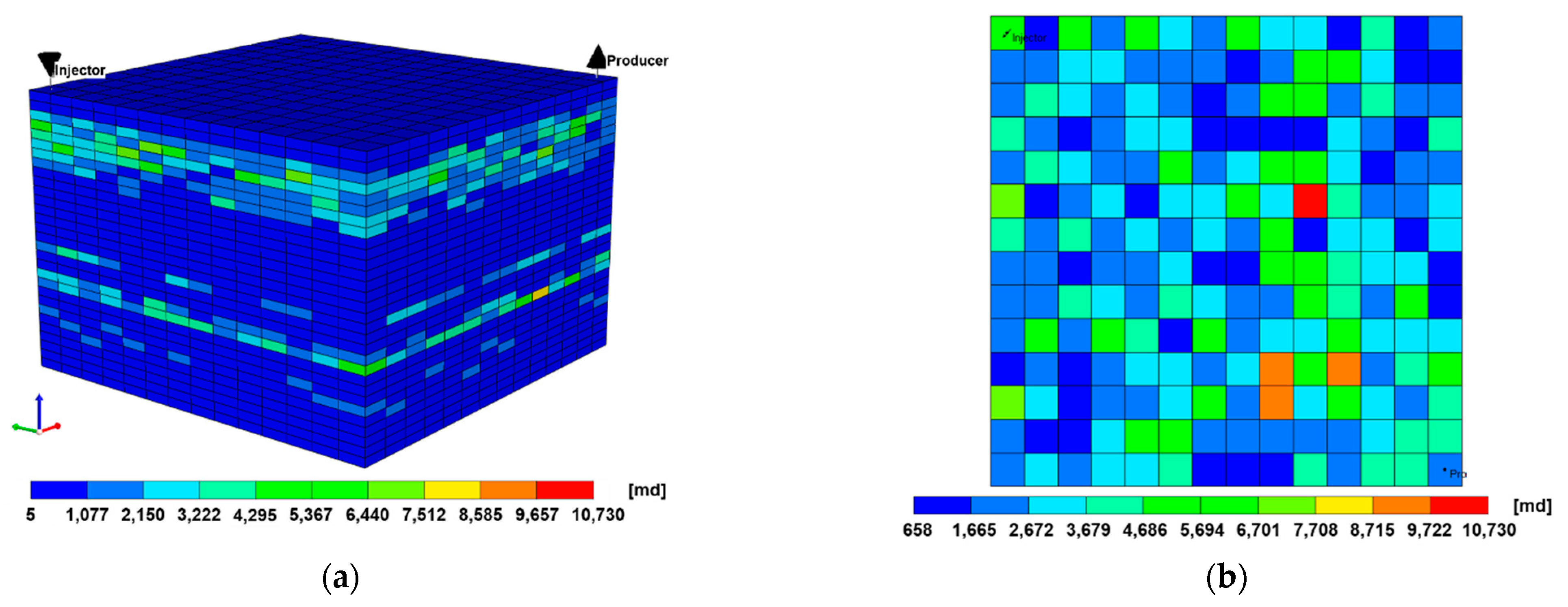
| Permeability Distribution | |
|---|---|
 | |
| Initial Conditions | |
| Size (ft3) | 200 × 10 × 96 |
| Grid | 20 × 1 × 30 |
| Average porosity | 0.148 |
| Average permeability (md) | 1535 |
| Depth (ft) | 5000 |
| Pressure (psi) | 2500 |
| Temperature (°F) | 100 |
| Parameter Range | Optimum Value | |
|---|---|---|
| Sucrose concentration (mole fraction) | 0.001–0.01 | 0.00235 |
| Treatment period (weeks) | 4–12 | 12 |
| Injection rate (bbl/day) | 10–100 | 100 |
| Injection temperature (°F) | 50–100 | 82 |
| Injection salinity (%) | 0–3 | 0 |
Publisher’s Note: MDPI stays neutral with regard to jurisdictional claims in published maps and institutional affiliations. |
© 2021 by the authors. Licensee MDPI, Basel, Switzerland. This article is an open access article distributed under the terms and conditions of the Creative Commons Attribution (CC BY) license (http://creativecommons.org/licenses/by/4.0/).
Share and Cite
Jeong, M.S.; Lee, Y.W.; Lee, H.S.; Lee, K.S. Simulation-Based Optimization of Microbial Enhanced Oil Recovery with a Model Integrating Temperature, Pressure, and Salinity Effects. Energies 2021, 14, 1131. https://doi.org/10.3390/en14041131
Jeong MS, Lee YW, Lee HS, Lee KS. Simulation-Based Optimization of Microbial Enhanced Oil Recovery with a Model Integrating Temperature, Pressure, and Salinity Effects. Energies. 2021; 14(4):1131. https://doi.org/10.3390/en14041131
Chicago/Turabian StyleJeong, Moon Sik, Young Woo Lee, Hye Seung Lee, and Kun Sang Lee. 2021. "Simulation-Based Optimization of Microbial Enhanced Oil Recovery with a Model Integrating Temperature, Pressure, and Salinity Effects" Energies 14, no. 4: 1131. https://doi.org/10.3390/en14041131
APA StyleJeong, M. S., Lee, Y. W., Lee, H. S., & Lee, K. S. (2021). Simulation-Based Optimization of Microbial Enhanced Oil Recovery with a Model Integrating Temperature, Pressure, and Salinity Effects. Energies, 14(4), 1131. https://doi.org/10.3390/en14041131