Article

Multivariate SCADA Data Analysis Methods for Real-World Wind Turbine Power Curve Monitoring

1
Department of Engineering, University of Perugia, 06125 Perugia, Italy
2
ENGIE Italia, Via Chiese, 20126 Milano, Italy
*
Author to whom correspondence should be addressed.
Energies 2021, 14(4), 1105; https://doi.org/10.3390/en14041105
Submission received: 10 February 2021 / Revised: 15 February 2021 / Accepted: 16 February 2021 / Published: 19 February 2021
(This article belongs to the Special Issue Wind Turbine Monitoring through Operation Data Analysis)

Abstract

:
Due to the stochastic nature of the source, wind turbines operate under non-stationary conditions and the extracted power depends non-trivially on ambient conditions and working parameters. It is therefore difficult to establish a normal behavior model for monitoring the performance of a wind turbine and the most employed approach is to be driven by data. The power curve of a wind turbine is the relation between the wind intensity and the extracted power and is widely employed for monitoring wind turbine performance. On the grounds of the above considerations, a recent trend regarding wind turbine power curve analysis consists of the incorporation of the main working parameters (as, for example, the rotor speed or the blade pitch) as input variables of a multivariate regression whose target is the power. In this study, a method for multivariate wind turbine power curve analysis is proposed: it is based on sequential features selection, which employs Support Vector Regression with Gaussian Kernel. One of the most innovative aspects of this study is that the set of possible covariates includes also minimum, maximum and standard deviation of the most important environmental and operational variables. Three test cases of practical interest are contemplated: a Senvion MM92, a Vestas V90 and a Vestas V117 wind turbines owned by the ENGIE Italia company. It is shown that the selection of the covariates depends remarkably on the wind turbine model and this aspect should therefore be taken in consideration in order to customize the data-driven monitoring of the power curve. The obtained error metrics are competitive and in general lower with respect to the state of the art in the literature. Furthermore, minimum, maximum and standard deviation of the main environmental and operation variables are abundantly selected by the feature selection algorithm: this result indicates that the richness of the measurement channels contained in wind turbine Supervisory Control And Data Acquisition (SCADA) data sets should be exploited for monitoring the performance as reliably as possible.

1. Introduction

Wind turbines operate under non-stationary conditions, because of the stochastic nature of the source [1,2], and the extracted power has a complex dependence on environmental conditions [3,4], on the control [5], on the health status [6] and on the age of the machine [7,8,9].
A further critical point regards the quality of the wind intensity measurements: despite there have been progresses in this regard recently, the standard in industrial wind farms is that cup anemometers are mounted behind the rotor span and the undisturbed wind speed is reconstructed through a nacelle transfer function. It is widely recognized that the nacelle transfer function is definitely site-dependent because it is affected by the turbulence intensity [10] and by the wind shear [11].
Based on these considerations, it is comprehensible that the design curves (thrust and power coefficient) of wind turbines provided by wind turbine manufacturers are representative of the performance which should be expected on site only within a certain extent. A more consistent approach is to be driven by data in the construction of reliable normal behavior models for the performance of wind turbines, but this is definitely a complex task. In this regard, an important turning point has been the development and the ubiquitous diffusion of Supervisory Control And Data Acquisition (SCADA) control systems, storing (typically with ten minutes of sampling time) a vast set of environmental, operational, thermal and electrical measurements. The use of SCADA data [12,13,14,15,16,17] therefore enables the possibility that the normal behavior models [18,19] are data-driven and therefore custom for each model type, site, wind turbine.
It is commonly accepted that the power curve [20,21,22,23,24,25,26,27] is a fundamental tool for wind turbine performance analysis because it is the representation of the power output as a function of the source (wind intensity). The International Electrotechnical Commission (IEC) [28] has recommended standards for the analysis of the power curve, which are particularly intuitive: the so-called binning method consists of grouping data per wind speed interval of 0.5 or 1 m/s and of averaging power measurements for each bin. By doing this, an average curve is obtained, against which it is possible to compare the observations. This methodology might be simplistic and for this reason a vast amount of scientific literature has been devoted to the improvement of the regression between wind intensity and power output: see [29] for a comprehensive review about the subject.
Yet, the above approach has intrinsic limitations: a regression between wind speed and power consists of finding the curve of best fit to observed measurements but, if the observations have a high variance, the improvement of such type of regression can reproduce it very partially: it is definitely more promising to incorporate in the model some additional information which allows reproducing more faithfully the real-world dispersion of the measurements. For this reason, a recent line of research in wind energy literature regards multivariate methodologies for the analysis of wind turbine power curves. There are no definite standards in this regard and the main issue deals with the selection of the further input variables, in addition to the wind speed. The basis for the selection of the input variables is the dependence of the power P of a wind turbine on environmental and operation variables, which can be expressed as in Equation (1):
P = 1 2 π R 2 ρ v 3 C p β , λ ,
where P is the produced power and depends on the rotor radius R, the air density ρ , the wind speed v and the power factor C p , which is a function of the blade pitch angle β and of the tip-speed ratio λ (or, in other words, of the rotational speed ω ).
In the following, a literature review about wind turbine multivariate power curve analysis is reported. To the best of the authors’ knowledge, the first study dealing with this topic is [30]: wind direction and ambient temperature are included as input variables and several regression methodologies are explored. In [31], SCADA data and meteorological mast data are combined for multivariate wind turbine power curve regression: the additional covariates are wind direction, humidity, turbulence intensity, wind shear. The regression type is an additive multivariate conditional kernel density estimation model, because of its capability of including additional input variables. In [32], the multivariate models employ wind direction, yaw error, blade pitch and rotor speed in addition to the wind speed. The inclusion of the yaw error is particularly interesting because aerodynamic considerations suggest that the power P extracted by a wind turbine depends on the yaw error γ through a cos 3 law [33]. In [34], the additional input variables are air density, turbulence intensity, wind direction and yaw error; in [35], the unique additional covariate is given by the wind direction. In [36], the analysis is focused on the incorporation of air density into the power curve. In [37], gaussian process models are analyzed and it is inquired if it is more convenient to add the rotor speed or the blade pitch to the model: the conclusion is that the rotor speed is the most appropriate working parameter for modelling the power of a wind turbine. In [38], the covariates include air density, blade pitch angle, rotor speed and wind direction; in [39], wind direction and blade pitch are incorporated in the model. In [40], the additional covariates are rotor speed, yaw error and an internal sub-component temperature.
On the grounds of the above discussion, it arises that there are at least two aspects which are overlooked and to which the present study aims at contributing innovatively:
  • the methodology for the input variables selection;
  • the exploitation of the information contained in the SCADA data sets.
In regard to the latter point, it should be noticed that the SCADA control systems of the wind turbines record and store average, minimum, maximum and standard deviation of each channel in the sampling time interval (which is typically ten minutes). Up to now, only the average values have been employed for wind turbine power curve modelling: the intuition of using as well minimum, maximum and standard deviation of the input variables has been explored only in [41] for other operation curves [42,43] of interest for wind turbine power monitoring, which are rotor speed—power, generator speed—power and blade pitch—power. The rationale for exploring this possibility is that these additional covariates might give information about the variability of the wind turbine behavior in the sampling time and therefore the resulting simulated curve might be more similar to the real-world one.
Another innovative point of the present study is that a large set of possible covariates is employed and the most appropriate for the regression are selected automatically through a sequential features selection algorithm [44], while in the vast majority of studies available in the literature the input variables are selected basing on plausibility and on reasoning similar to Equation (1): actually, an example of features selection algorithm applied to this kind of problems is given in [45], but the model structure is simplified (polynomial regression) with respect to the one employed in this study. The regression type selected for this study is actually the Support Vector with Gaussian Kernel [46], because it has been observed to be adequate for non-linear problems in wind energy applications [8,41,47,48].
A meaningful point of this study is that three test cases have been analyzed, dealing with three different wind turbine models which are of interest for wind energy practitioners because of their widespread diffusion: courtesy of the ENGIE Italia, data have been analyzed from a Senvion MM92, a Vestas V90 and a Vestas V117 wind turbines sited in southern Italy. Actually, the present study constitutes a scientific collaboration between academia and industry: University of Perugia and ENGIE Italia. There is a rationale in this selection, which is the “real-world” approach of this study: industrial wind turbines have been selected and these are of course characterized by the typical critical points of the real-world application of energy systems, which are the complexity of the environment in which they are sited; the possible curtailments and grid limitations affecting the operation; the possible lack of information about the long-term history of the wind turbines. It is therefore a qualifying aspect of this study that, despite the above issues, it has been possible to successfully apply a high-level data analysis methodology.
The motivations of the present study are confirmed by the results which have been achieved, which summarizing are the following:
  • the minimum, maximum and standard deviation of the most meaningful environmental and operation variables are abundantly selected by the features selection algorithm;
  • the selection of the input variables heavily depends on the wind turbine model and it is therefore supported that data-driven power curve models should be customized on the wind turbines of interest;
  • by employing the selected input variables and the selected regression type, it is possible to achieve error metrics which are in general lower than the state of the art in the literature and are shown to be lower than those given by an appropriate benchmark model. This is the qualifying point for this kind of approaches because the lower the error metrics and the higher the capability of recognizing performance deviations with respect to the normal: in this regard, the data-driven methods prove to be superior to the design curves of the wind turbines.
The organization of this work is as follows: Section 2 is devoted to the description of the test cases and of the data sets, in Section 3 the methods are described; the results are collected and discussed in Section 4; finally, conclusions are drawn in Section 5.

2. Test Cases and Data Sets

Three test cases have been selected for this work, from industrial wind farms owned by the ENGIE Italia company:
  • a Senvion MM92;
  • a Vestas V90;
  • a Vestas V117.
The main features of the test case wind turbines are summarized in Table 1 and a snapshot of one wind farm is reported in Figure 1.
Two years of data (10 min of sampling time) for each wind turbine have been analyzed, which are indicated in Table 1. The data have been downloaded from the SCADA Open Platform Communications Data Access (OPC-DA) server of the proprietary system of the wind turbines and consequently shared to the University of Perugia in the form of text files. The measurements at disposal are:
  • Wind speed v (m/s) (average, minimum, maximum, standard deviation);
  • Power P (kW) (average);
  • Blade pitch β ( ) (average, minimum, maximum, standard deviation);
  • Generator speed ω (rpm) (average, minimum, maximum, standard deviation);
  • Rotor speed Ω (rpm) (average, minimum, maximum, standard deviation);
  • Ambient temperature T ( C ) (average);
  • Run time counter R (s).
As anticipated in Section 1, one of the innovative points of the present study is that minimum, maximum and standard deviation of the main possible input variables are included. Most studies dealing with multivariate models for wind turbine power curve employ rotor speed and blade pitch as input variables: this is plausible because these operation variables, as discussed for example in [37,41], provide meaningful information about the working point of the wind turbine and therefore about the power which is expected to be extracted. On the grounds of the considerations in [9], in this work also the generator speed has been included because the efficiency of the generator can have a non-negligible impact on the performance of a wind turbine.
The data have been appropriately pre-processed as follows:
  • filter using the run time counter, requesting production for 600 s out 600;
  • filter below rated power (approximately v 13 );
  • since grid curtailments are operated by forcing the wind turbine to pitch anomalously, these are filtered out by removing outliers with respect to the average wind speed—blade pitch curve ( 3 of tolerance).
The dependence of the power P on the ambient temperature is taken into account by renormalizing as indicated in Equation (2):
v c = v ρ ρ r e f 1 3 ,
with (Equation (3))
ρ = ρ r e f T r e f T .
In Equations (2) and (3), ρ is the air density measured on site, ρ r e f is the air density in standard conditions (1.225 kg / m 3 ), T r e f is the standard absolute temperature (288.15 K), T is the absolute temperature measured on site, v c is the corrected wind speed, v is the estimate of undisturbed wind speed provided by the wind turbine nacelle anemometer.
An example of power curve scatter upon data filtering is reported in Figure 2 for the Senvion MM92 case.

3. Methods

The objective of this study is formulating and applying an appropriate regression for the power P of the test cases wind turbines, as a function of the input variables matrix X . An important point of this study is that the features selection is performed through a sequential algorithm, applying the selected type of regression at each iteration, which is Support Vector Regression with Gaussian Kernel [49].
Therefore, here on the principles of this kind of regression are described and, subsequently, the features selection algorithm is sketched and the selected features for each test case are listed. The notation is the following:
  • Y is the vector of measured output (power production P);
  • X is the matrix of covariates, which can be selected between
    • Renormalized wind speed v c (average);
    • Renormalized windspeed v c m i n (mimimum);
    • Renormalized wind speed v c m a x (maximum);
    • Renormalized wind speed v c σ (standard deviation);
    • Blade pitch β (average);
    • Blade pitch β m i n (mimimum);
    • Blade pitch β m a x (maximum);
    • Blade pitch β σ (standard deviation);
    • Generator speed ω (average);
    • Generator speed ω m i n (minimum);
    • Generator speed ω m a x (maximum);
    • Generator speed ω σ (standard deviation);
    • Rotor speed Ω (average);
    • Rotor speed Ω m i n (minimum);
    • Rotor speed Ω m a x (maximum);
    • Rotor speed Ω σ (standard deviation).
  • f ( X ) 
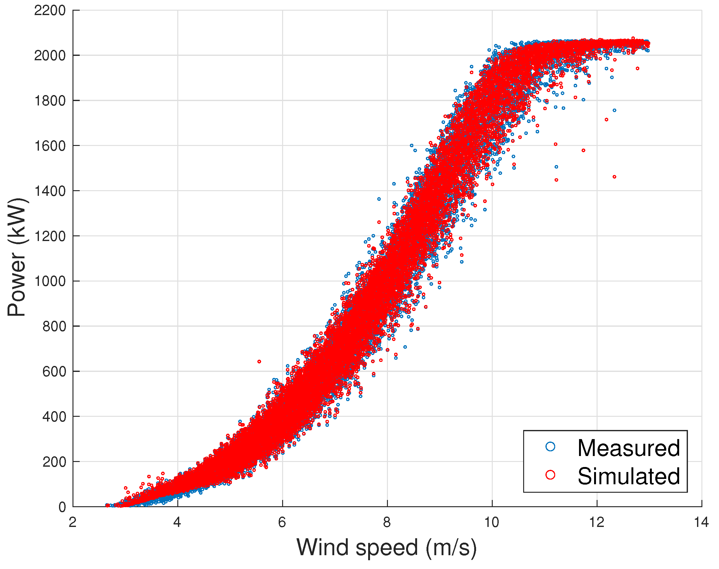
is the vector of simulated output, for given input variables X .
The principles of Support Vector Regression can be understood more clearly by starting from a linear model (Equation (4)):
f ( X ) = X β + b ,
where β are the coefficients of the regression, multiplying the columns corresponding to the covariates, and b are the intercept coefficients.
Given the matrix X of observed inputs, the Support Vector estimate of the β coefficients is obtained by requiring the optimization between two potentially conflicting targets:
  • the precision of the regression, which means that the absolute difference between the model estimate and the measurement should be lower than a threshold ϵ (Equation (5));
  • the flatness of the model, which means that the norm of the coefficients β β should be minimum. In one dimension, it means that regression line should be as close as possible to the x-axis.
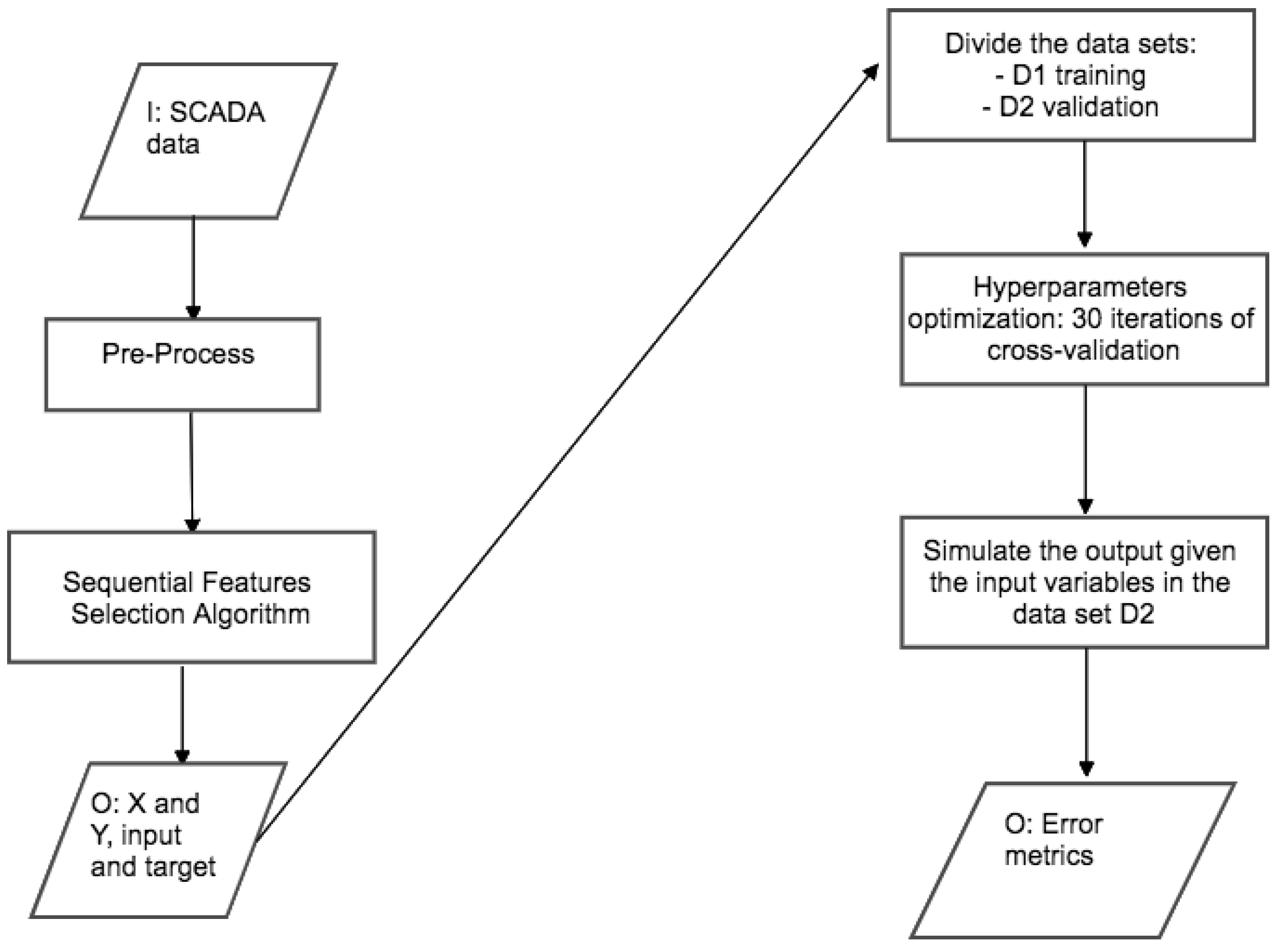
Y n X n β + b n ϵ .
This kind of optimization problems is typically rephrased in the Lagrange dual formulation. The function to minimize is L α (Equation (6)):
L α = 1 2 i = 1 N j = 1 N α i α i * α j α j * X i X j + ϵ i = 1 N α i + α i * + i = 1 N Y i α i * α i ,
with the constraints (Equation (7))
n = 1 N α n α n * = 0 0 α n C 0 α n * C ,
where C is the box constraint.
The Support Vector estimate of the regression coefficients is given in Equation (8):
β = n = 1 N α n α n * X n .
The name of the regression comes from the fact that potentially most of the coefficients α n or α n * in Equation (8) are zero and the non vanishing ones are associated to a support vector observation (which is a row of the X matrix).
Once the model has been trained and the coefficients α n and α n * have been set, it is possible to simulate the output f ( X ) given the input variables matrix X , as in Equation (9):
f ( X ) = n = 1 N α n α n * X n X + b .
The non-linear Support Vector Regression is obtained by replacing the products between the observations matrix with a non-linear Kernel function (Equation (10)):
G X 1 , X 2 = φ X 1 φ X 2 ,
where φ is a transformation mapping the X observations into the kernel space.
A Gaussian Kernel selection is given in Equation (11) and is widely employed for non-linear problems:
G X i , X j = e κ X i X j 2 ,
where κ is the kernel scale. Then Equation (6) becomes Equation (12):
L α = 1 2 i = 1 N j = 1 N α i α i * α j α j * G X i , X j + ϵ i = 1 N α i + α i * + i = 1 N Y i α i * α i ,
and Equation (9) for predicting rewrites as in Equation (13):
f ( X ) = n = 1 N α n α n * G X n , X + b .
In practice, for a non-linear model the support vector observations, which multiply the non-vanishing α or α * , are mapped into the kernel space which weights them according to the transformation map: in the case of Gaussian Kernel, the map is a gaussian norm.
The above type of regression is employed at each run by the sequential features algorithm employed in this study, which proceeds as follows:
  • the matrix X , containing the sixteen possible regressors listed above, and the vector Y of power output are passed to a sequence of Support Vector Regressions;
  • starting from an empty X matrix, the algorithm adds once at a time each possible input variable (i.e., each column), performs a 10-fold cross-validation of the regression and estimates the loss function;
  • the regressor associated to the lowest value of the loss function is selected as input of the model;
  • sequentially, each other possible regressor is added once at a time, the cross-validation is performed, the loss function is estimated;
  • if, by adding a regressor, there is no more improvement in the loss function, the algorithm stops and returns the input variables selected up to this step;
  • else, the algorithm adds to the input variables selection the regressor which diminishes most the loss function and the sequence proceeds.
It should be noticed that the average renormalized wind speed v c is the regressor which is added for first in each test case. This is coherent with what observed in [32], as regards the fact that the wind speed explains up to 97% of the variance of the power P.
Once the input variables have been selected, the data set at disposal is divided as follows:
  • a random 50% selection is used for training the model and is noted as D1;
  • the remainder 50% (hence named D2) is used for evaluating the goodness of the regression, by evaluating the out-of-sample error metrics.
The training phase consists of an automatic optimization of the model hyper-parameters by means of 30 model runs.
Given the measurements Y ( X ) for the validation data set D2 and the model estimates f ( X ) , the set of residuals is defined in Equation (5):
R ( X ) = Y ( X ) f ( X ) .
The error metrics which are employed in this work are the most typical ones and are the Mean Absolute Error (MAE), the Mean Absolute Percentage Error (MAPE) and the Root Mean Squar Error (RMSE). The MAE is defined in Equation (15):
M A E = 1 N R ( X ) ,
where N is the number of samples in the validation data set. The MAPE is defined in Equation (16):
M A P E = 100 N R ( X ) Y ( X )
and the R M S E is defined in Equation (17):
R M S E = R ( X ) R ¯ 2 N ,
where R ¯ is the average residual in the data set D2.
The structure of the proposed methodology is summarized in the block diagram of Figure 3.
In order to provide a comparison against a benchmark in line with the consolidated findings in the literature, the same kind of regression has been set up for a reduced model M r e d taking as input variables the average renormalized wind speed v c , the average blade pitch β and the average rotor speed Ω . The error metrics of this reduced model are compared against the model proposed in this study, which is denoted as M.

4. Results

The results of the automatic features selection are reported in Table 2, about which several comments arise:
  • The covariates which are selected for all the test cases are the average wind speed v c and the standard deviation of the wind speed v c σ . This indicates that it is fundamental to incorporate in the model information regarding the turbulence intensity on site and this results support the idea of this study to include minimum, maximum and standard deviation of the main possible input variables.
  • A large number of covariates is selected for each test case (8 or 9) and the minimum, maximum and standard deviation of the variables are the most selected: the maximum number of average values which are selected is 3. This strongly supports the intuition of this work.
  • There is a remarkable difference in the variables selection between the Senvion MM92 and the two Vestas test cases: for the Senvion MM92, 5 rotational speed variables and 1 blade pitch variable are selected, while for the Vestas wind turbines, 1 rotational speed variable and 4 blade pitch variables are selected. This is likely due to the different type of control of the wind turbine: Senvion MM92 has electric pitch control, while the Vestas wind turbines have hydraulic pitch control. This result supports that the multivariate regression for the power curve should be custom, depending on the wind turbine model, despite in general it is definitely reasonable that blade pitch and rotational speed are very important working parameters.

4.1. Senvion MM92

In Figure 4, a scatter plot is reported for the measured and simulated power curves in the validation data set D2. From this Figure, it is possible to appreciate qualitatively that the simulated curve reproduces reliably the observed one.
In Table 3, the error metrics are reported for the selected model of Table 2 and for the benchmark model M r e d . It arises that the error metrics for the model individuated in this work are lower with respect to the benchmark model: in particular, the decrease regards the M A E and the R M S E (diminishing of the 27% and 30% respectively). The decrease of the M A P E when adopting the proposed model is instead lower and this can be interpreted in light of Figure 5, where the residuals between measurements and model estimates are plotted after being averaged in interval of the 10% of the rated power: it arises that the main improvement provided by the M model regards the behavior for moderate—high power and this explains why the M A E and R M S E diminish more than a percentage error like the M A P E .

4.2. Vestas V90

In Figure 6, the measured and simulated power curves are reported for the Vestas V90 test case. The error metrics for the M and M r e d models are reported in Table 4: adopting the model proposed in this work, the M A E decreases of the 17% with respect to M r e d and the R M S E of the 12.9%. By analyzing Figure 7, it arises that the model proposed in this work is better than the benchmark M r e d especially approaching rated power. This can likely be explained as due to the fact that the behavior of the pitch is the most influential parameter in that working region: in [40], it was noticed that this aspect is particularly difficult to reproduce with a multivariate regression. Evidently, the input variables selection of Table 2, which consists for this test case of employing all the available information as regards the blade pitch (average, minimum, maximum, standard deviation), provides good results near rated power.

4.3. Vestas V117

In Figure 8, the scatter plot is reported for the measured and simulated power curve during the validation data set D2. The error metrics for the proposed model M and for the benchmark model M r e d are reported in Table 5. It arises that the proposed model provides a M A E 20% lower, a R M S E 16.5% lower and a M A P E 22% lower. In particular, for power higher than 2 MW, the proposed model provides lower absolute value of the residuals, as can be hinted from Figure 9: this can likely be interpreted, similarly to the Vestas V90 test case (Section 4.2), as the effect of the use of all the available information as regards the blade pitch.

4.4. Discussion

  • The first observation arising from Section 4.1, Section 4.2 and Section 4.3 is that the models proposed in this work, whose input variables selections are reported in Table 2, provide lower error metrics with respect to the selected benchmark model. The error metrics decrease from M r e d to M is approximately in the order of 20–30%.
  • The error metrics which have been achieved are slightly different, depending on the test case: for the Senvion MM92, the M A E is 0.87% of the rated power, for the Vestas V90 it is 1.28% of the rated power and for the Vestas V117 it is 1.41% of the rated power.
  • The above results are competitive and in general lower with respect to the state of the art in the literature. In [39], the obtained M A E is in the order of 1.5% of the rated power, in [37] a M A E in the order of 1.1% of the rated power is obtained, in [35] (dealing with the Vestas V90 as in the present work) the M A E is approximately 1.45% of the rated power.
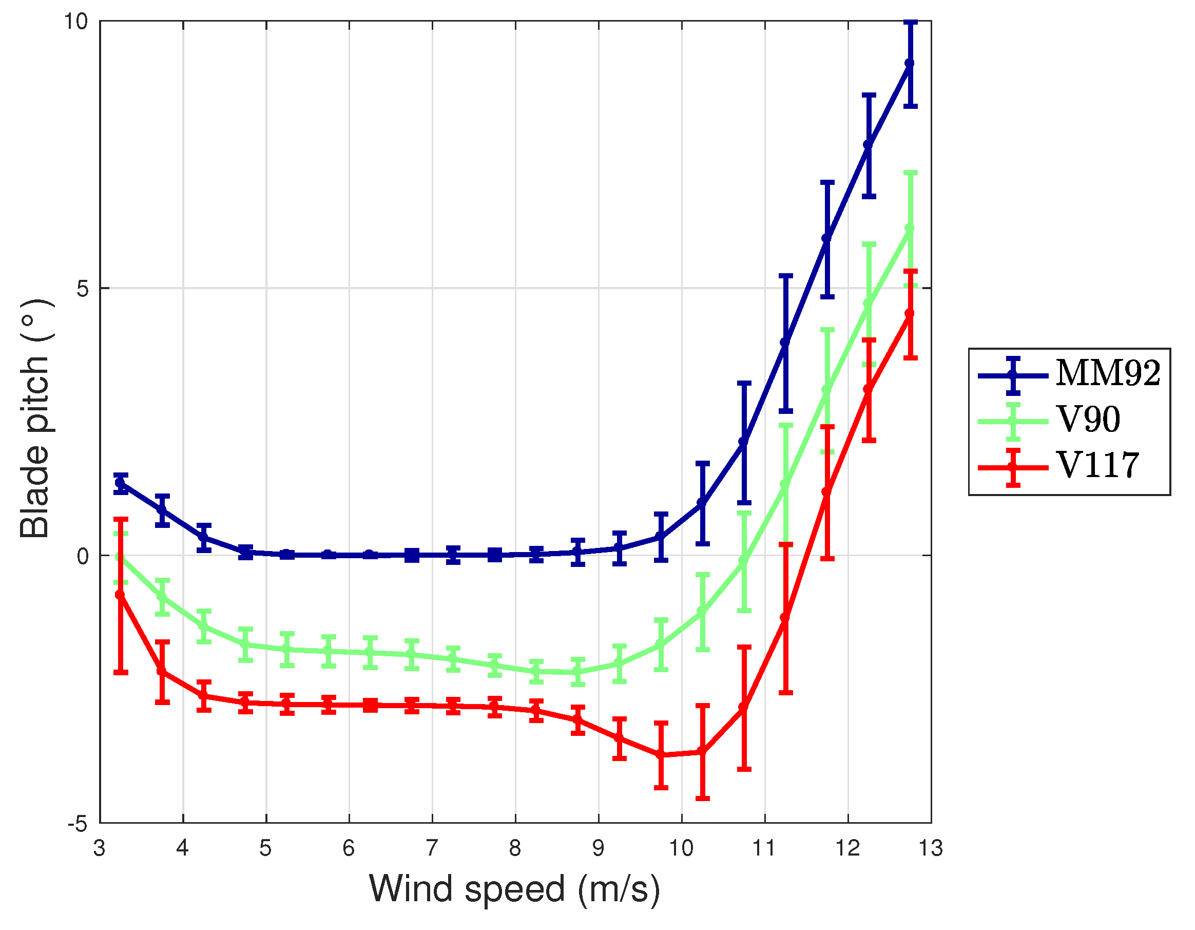
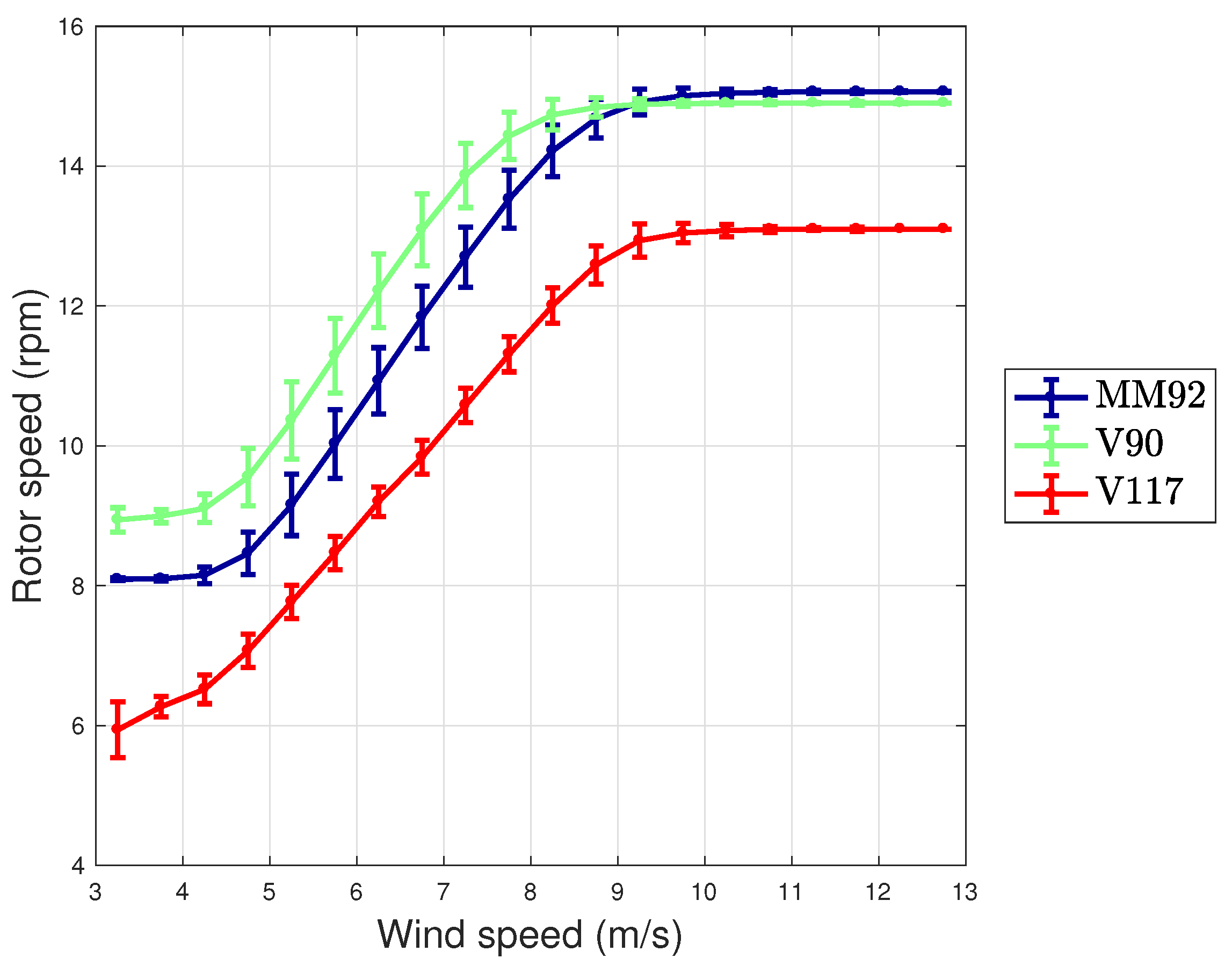
  • The case of Vestas V117 deserves a further discussion, because it is the test case with largest rotor diameter and highest rated power available in the literature, to the best of the authors’ knowledge. The error metrics for this test case resulted to be slightly highest with respect to the other test cases of this work, which have 2 MW of rated power. In order to understand the possible critical points, in Figure 10 and Figure 11, the average wind speed—blade pitch and wind speed—rotor speed curves [42] are reported for each test case. It arises that the behavior of the blade pitch for the Vestas V117 is more critical because there is higher variability near the cut-in and approaching rated power. From Figure 10, it also arises that the wind turbine displaying a more regular pitch behavior is the Senvion MMM92 and this likely explains why for this test case the regression (Table 2) employs only one input variable related to the blade pitch. Recall that, as reported in Table 1, the Senvion MM92 has electric pitch control, while the Vestas wind turbines have hydraulic pitch control [50]. Furthermore, from Figure 11, it arises that the the Vestas V117 wind turbine has a lower variability in the behavior of the rotor speed and this likely contributes to explain why the rotational speed variables are less important for this wind turbine.
  • Potentially, there are no drawbacks regarding the extension of the proposed methodology to other models of wind turbines. It should be noticed that, in general, the older the wind turbines and the less rich are the SCADA data sets. As a rule of thumb, it can be stated that the benefits of the proposed approach can be appreciated when applied to wind turbines of the generation of Vestas V52 [51] up to the latest models in the market. For wind turbines like the Vestas V52, the model could in particular be useful for a long term analysis of the performance trend in the context of the assessment of performance decline with age. In relation to the application of the method to the latest models in the market, of increasing rotor size, it should be noticed that the exploitation of all the available wind intensity sensors could be decisive for further diminishing the error metrics.

5. Conclusions

The present study has been devoted to the formulation of a data-driven methodology for the multivariate modelling of wind turbine power curves.
Some innovative points of this study are qualifying:
  • The SCADA data at disposal have been exploited more in depth with respect to the state of the art in the literature, because minimum, maximum and standard deviation in the sampling time of the main environmental and working variables have been included as possible covariates of the model for the power. In the literature, the typical choice is employing only the average values.
  • A sequential features selection algorithm has been employed in order to identify the most appropriate covariates for the regression. The algorithm starts from an empty set and adds each covariate one at a time, selecting iteratively the one which leads to a lower error metric, and stopping when there is no improvement in adding further inputs.
Three test cases of particular practical interest have been analyzed, from industrial wind farms owned by the ENGIE Italia company: a Senvion MM92, a Vestas V90 and a Vestas V117.
The innovative approach, in conjunction with the analysis of three different wind turbine models, has led to significant results:
  • The inclusion of minimum, maximum and standard deviation of the main variables as possible regressors is meaningful: from Table 2, where the features selection for three test cases is reported, it arises that the average values are only around 20% of the selected input variables.
  • There are some regular characteristics in the features selection of Table 2: the average wind speed is the most important input, the standard deviation of the wind speed is the second most important, at least a variable related to rotational speed and to blade pitch is selected. The number of selected features is quite high (8, 9) with respect to most models in the literature, which typically employ average wind speed, blade pitch, rotor speed and possibly the yaw error.
  • There are differences between the features selected for the various test cases: for the Senvion MM92 technology, the information related to rotational speed results being more meaningful, while for the Vestas technology all the measurements regarding the blade pitch are included in the models. This could probably be interpreted in light of the control of the wind turbines (Figure 10).
  • For each test case, the error metrics obtained with the regression method proposed in this work are lower with respect to the state of the art in the literature and are considerably lower with respect to those obtained through a benchmark model employing average wind speed, blade pitch and rotor speed.
In light of the above considerations, the lesson is that the use of an automatic features selection algorithm is an important point of strength for multivariate approaches to the wind turbine power curve, because it allows identifying the most meaningful variables explaining the variance of the extracted power. This is particularly important because, as Table 2 suggests, it is likely that for each wind turbine technology there are preferable selections and in general it can be argued that the data-driven multivariate power curve regression should be custom.
A straightforward further direction of the present study is an in-depth analysis of how the features selection and the regression error metrics depend on the conditions measured at different sites: it would therefore be interesting to analyze several wind turbines of the same model, placed in very different environments (onshore flat terrain, onshore complex terrain, offshore, high turbulence, low turbulence, high wind shear, low wind shear, etc.).
The results of this study, as well as most of the studies regarding this topic in the literature, indicate that the rotational speed and the blade pitch are very meaningful working parameters of wind turbine. It does not come as a surprise, therefore, that the idea of formulating a rotor equivalent wind speed has been conceived [52,53] and in [41] the issue has been posed if it possible to similarly define a pitch equivalent wind speed when the wind turbine operates at partial aerodynamic load. Nevertheless, this study indicates that in general the information contained in the SCADA data sets is considerably under-exploited for multivariate power curve regression: it would therefore be interesting to inquire if thermal, hydraulic, electric variables typically included in the SCADA data sets could be helpful as further input variables. This issue is particularly relevant in the context of increasing wind turbine rotor size [54] because, as the V117 test case considered in this study indicates, a precise monitoring of wind turbine power curve could be more challenging as the size of the wind turbine increases.
The results of the present study suggest that it is possible to exploit in depth the SCADA data of wind turbines in order to diminish the error metrics for the normal behavior models used to evaluate performance: this could be applied not only to identify degradation but, on the other way round, as well to quantify the actual improvement provided by aerodynamic and-or control wind turbine optimization technology [55,56], which typically weights few percents of production.
The proposed approach based on sequential features selection can potentially be employed also for classification, finalized to fault diagnosis [57] and health status assessment [58,59] through SCADA data analysis [60,61,62,63]: in particular, a reliable data-driven model of sub-component temperature can be particularly useful for the diagnosis of incoming gears and bearings faults [64] and it is possible that the approach of this study could be inspiring for this kind of application.
Finally, a practical development of the present study regards the collaboration between academia and industry and it is constituted by the automation of the methodology (data download from the OPC server, store of the historical data, data import and data analysis) through open access libraries (as, for example, in Python) which can be easily implemented and incorporated in the industrial practice.

Author Contributions

Conceptualization, D.A., F.C., A.L. and L.T.; Data curation, D.A. and A.L.; Formal analysis, D.A., F.C., A.L. and L.T.; Investigation, D.A.; Methodology, D.A.; Software, D.A.; Supervision, F.C. and L.T.; Validation, D.A., F.C., A.L. and L.T.; Writing—original draft, D.A.; Writing—review editing, D.A., F.C., A.L. and L.T. All authors have read and agreed to the published version of the manuscript.

Funding

This research received no external funding.

Conflicts of Interest

The authors declare no conflict of interest.

Abbreviations

The following abbreviations are used in this manuscript:
DAData Access
IECInternational Electrotechnical Commission
MAEMean Absolute Error
MAPEMean Absolute Percentage Error
OPCOpen Platform Communication
RMSERoot Mean Square Error
SCADASupervisory Control And Data Acquisition
SVRSupport Vector Regression

References

  1. Zhang, Y.; Pan, G.; Chen, B.; Han, J.; Zhao, Y.; Zhang, C. Short-term wind speed prediction model based on GA-ANN improved by VMD. Renew. Energy 2020, 156, 1373–1388. [Google Scholar] [CrossRef]
  2. Zhang, Y.; Zhao, Y.; Kong, C.; Chen, B. A new prediction method based on VMD-PRBF-ARMA-E model considering wind speed characteristic. Energy Convers. Manag. 2020, 203, 112254. [Google Scholar] [CrossRef]
  3. Wagner, R.; Antoniou, I.; Pedersen, S.M.; Courtney, M.S.; Jørgensen, H.E. The influence of the wind speed profile on wind turbine performance measurements. Wind. Energy Int. J. Prog. Appl. Wind. Power Convers. Technol. 2009, 12, 348–362. [Google Scholar] [CrossRef]
  4. Han, X.; Liu, D.; Xu, C.; Shen, W.Z. Atmospheric stability and topography effects on wind turbine performance and wake properties in complex terrain. Renew. Energy 2018, 126, 640–651. [Google Scholar] [CrossRef]
  5. Astolfi, D.; Castellani, F.; Natili, F. Wind turbine yaw control optimization and its impact on performance. Machines 2019, 7, 41. [Google Scholar] [CrossRef] [Green Version]
  6. Sequeira, C.; Pacheco, A.; Galego, P.; Gorbeña, E. Analysis of the efficiency of wind turbine gearboxes using the temperature variable. Renew. Energy 2019, 135, 465–472. [Google Scholar] [CrossRef]
  7. Dai, J.; Yang, W.; Cao, J.; Liu, D.; Long, X. Ageing assessment of a wind turbine over time by interpreting wind farm SCADA data. Renew. Energy 2018, 116, 199–208. [Google Scholar] [CrossRef] [Green Version]
  8. Byrne, R.; Astolfi, D.; Castellani, F.; Hewitt, N.J. A Study of Wind Turbine Performance Decline with Age through Operation Data Analysis. Energies 2020, 13, 2086. [Google Scholar] [CrossRef] [Green Version]
  9. Astolfi, D.; Byrne, R.; Castellani, F. Analysis of Wind Turbine Aging through Operation Curves. Energies 2020, 13, 5623. [Google Scholar] [CrossRef]
  10. Martin, C.M.S.; Lundquist, J.K.; Clifton, A.; Poulos, G.S.; Schreck, S.J. Atmospheric turbulence affects wind turbine nacelle transfer functions. Wind. Energy Sci. 2017, 2, 295–306. [Google Scholar] [CrossRef] [Green Version]
  11. Honrubia, A.; Vigueras-Rodríguez, A.; Gómez-Lázaro, E. The influence of turbulence and vertical wind profile in wind turbine power curve. In Progress in Turbulence and Wind Energy IV; Springer: Berlin/Heidelberg, Germany, 2012; pp. 251–254. [Google Scholar]
  12. Larios, D.F.; Personal, E.; Parejo, A.; García, S.; García, A.; Leon, C. Operational Simulation Environment for SCADA Integration of Renewable Resources. Energies 2020, 13, 1333. [Google Scholar] [CrossRef] [Green Version]
  13. Lee, S.H.; Huh, J.H. Optimal Location Recommendation System for Offshore Floating Wind Power Plant Using Big Data Analysis. In Advances in Computer Science and Ubiquitous Computing; Springer: Berlin/Heidelberg, Germany, 2021; pp. 583–590. [Google Scholar]
  14. Abdallah, I.; Dertimanis, V.; Mylonas, H.; Tatsis, K.; Chatzi, E.; Dervilis, N.; Worden, K.; Maguire, E. Fault diagnosis of wind turbine structures using decision tree learning algorithms with big data. In Proceedings of the European Safety and Reliability Conference, Trondheim, Norway, 17–21 June 2018; pp. 3053–3061. [Google Scholar]
  15. Castellani, F.; Garinei, A.; Terzi, L.; Astolfi, D.; Moretti, M.; Lombardi, A. A new data mining approach for power performance verification of an on-shore wind farm. Diagnostyka 2013, 14, 35–42. [Google Scholar]
  16. Astolfi, D.; Castellani, F.; Terzi, L. Mathematical methods for SCADA data mining of onshore wind farms: Performance evaluation and wake analysis. Wind. Eng. 2016, 40, 69–85. [Google Scholar] [CrossRef] [Green Version]
  17. Castellani, F.; Garinei, A.; Terzi, L.; Astolfi, D.; Gaudiosi, M. Improving windfarm operation practice through numerical modelling and supervisory control and data acquisition data analysis. IET Renew. Power Gener. 2014, 8, 367–379. [Google Scholar] [CrossRef]
  18. Schlechtingen, M.; Santos, I.F.; Achiche, S. Wind turbine condition monitoring based on SCADA data using normal behavior models. Part 1: System description. Appl. Soft Comput. 2013, 13, 259–270. [Google Scholar] [CrossRef]
  19. Schlechtingen, M.; Santos, I.F. Wind turbine condition monitoring based on SCADA data using normal behavior models. Part 2: Application examples. Appl. Soft Comput. 2014, 14, 447–460. [Google Scholar] [CrossRef]
  20. Pandit, R.K.; Infield, D.; Kolios, A. Comparison of advanced non-parametric models for wind turbine power curves. IET Renew. Power Gener. 2019, 13, 1503–1510. [Google Scholar] [CrossRef] [Green Version]
  21. Saint-Drenan, Y.M.; Besseau, R.; Jansen, M.; Staffell, I.; Troccoli, A.; Dubus, L.; Schmidt, J.; Gruber, K.; Simões, S.G.; Heier, S. A parametric model for wind turbine power curves incorporating environmental conditions. Renew. Energy 2020, 157, 754–768. [Google Scholar] [CrossRef]
  22. Wang, Y.; Li, Y.; Zou, R.; Foley, A.M.; Al Kez, D.; Song, D.; Hu, Q.; Srinivasan, D. Sparse Heteroscedastic Multiple Spline Regression Models for Wind Turbine Power Curve Modeling. IEEE Trans. Sustain. Energy 2020, 12, 191–201. [Google Scholar] [CrossRef]
  23. Mehrjoo, M.; Jozani, M.J.; Pawlak, M. Wind turbine power curve modeling for reliable power prediction using monotonic regression. Renew. Energy 2020, 147, 214–222. [Google Scholar] [CrossRef]
  24. Helbing, G.; Ritter, M. Improving wind turbine power curve monitoring with standardisation. Renew. Energy 2020, 145, 1040–1048. [Google Scholar] [CrossRef]
  25. Rogers, T.; Gardner, P.; Dervilis, N.; Worden, K.; Maguire, A.; Papatheou, E.; Cross, E. Probabilistic modelling of wind turbine power curves with application of heteroscedastic Gaussian Process regression. Renew. Energy 2020, 148, 1124–1136. [Google Scholar] [CrossRef]
  26. Yun, E.; Hur, J. Probabilistic estimation model of power curve to enhance power output forecasting of wind generating resources. Energy 2021, 223, 120000. [Google Scholar] [CrossRef]
  27. Pandit, R.; Kolios, A. SCADA Data-Based Support Vector Machine Wind Turbine Power Curve Uncertainty Estimation and Its Comparative Studies. Appl. Sci. 2020, 10, 8685. [Google Scholar] [CrossRef]
  28. International Electrotechnical Commission (IEC). Power Performance Measurements of Electricity Producing Wind Turbines; Technical Report 61400–12; International Electrotechnical Commission: Geneva, Switzerland, 2005. [Google Scholar]
  29. Wang, Y.; Hu, Q.; Li, L.; Foley, A.M.; Srinivasan, D. Approaches to wind power curve modeling: A review and discussion. Renew. Sustain. Energy Rev. 2019, 116, 109422. [Google Scholar] [CrossRef]
  30. Schlechtingen, M.; Santos, I.F.; Achiche, S. Using data-mining approaches for wind turbine power curve monitoring: A comparative study. IEEE Trans. Sustain. Energy 2013, 4, 671–679. [Google Scholar] [CrossRef]
  31. Lee, G.; Ding, Y.; Genton, M.G.; Xie, L. Power curve estimation with multivariate environmental factors for inland and offshore wind farms. J. Am. Stat. Assoc. 2015, 110, 56–67. [Google Scholar] [CrossRef] [Green Version]
  32. Janssens, O.; Noppe, N.; Devriendt, C.; Van de Walle, R.; Van Hoecke, S. Data-driven multivariate power curve modeling of offshore wind turbines. Eng. Appl. Artif. Intell. 2016, 55, 331–338. [Google Scholar] [CrossRef]
  33. Burton, T.; Jenkins, N.; Sharpe, D.; Bossanyi, E. Wind Energy Handbook; John Wiley & Sons: Chicester, UK, 2011. [Google Scholar]
  34. Pelletier, F.; Masson, C.; Tahan, A. Wind turbine power curve modelling using artificial neural network. Renew. Energy 2016, 89, 207–214. [Google Scholar] [CrossRef]
  35. Manobel, B.; Sehnke, F.; Lazzús, J.A.; Salfate, I.; Felder, M.; Montecinos, S. Wind turbine power curve modeling based on Gaussian processes and artificial neural networks. Renew. Energy 2018, 125, 1015–1020. [Google Scholar] [CrossRef]
  36. Pandit, R.K.; Infield, D.; Carroll, J. Incorporating air density into a Gaussian process wind turbine power curve model for improving fitting accuracy. Wind Energy 2019, 22, 302–315. [Google Scholar] [CrossRef] [Green Version]
  37. Pandit, R.K.; Infield, D.; Kolios, A. Gaussian process power curve models incorporating wind turbine operational variables. Energy Rep. 2020, 6, 1658–1669. [Google Scholar] [CrossRef]
  38. Shetty, R.P.; Sathyabhama, A.; Pai, P.S. Comparison of modeling methods for wind power prediction: A critical study. Front. Energy 2020, 14, 347–358. [Google Scholar] [CrossRef]
  39. Karamichailidou, D.; Kaloutsa, V.; Alexandridis, A. Wind turbine power curve modeling using radial basis function neural networks and tabu search. Renew. Energy 2020, 163, 2137–2152. [Google Scholar] [CrossRef]
  40. Astolfi, D.; Castellani, F.; Natili, F. Wind Turbine Multivariate Power Modeling Techniques for Control and Monitoring Purposes. J. Dyn. Syst. Meas. Control 2021, 143, 034501. [Google Scholar] [CrossRef]
  41. Astolfi, D. Wind Turbine Operation Curves Modelling Techniques. Electronics 2021, 10, 269. [Google Scholar] [CrossRef]
  42. Pandit, R.K.; Infield, D. Comparative assessments of binned and support vector regression-based blade pitch curve of a wind turbine for the purpose of condition monitoring. Int. J. Energy Environ. Eng. 2019, 10, 181–188. [Google Scholar] [CrossRef] [Green Version]
  43. Pandit, R.; Infield, D. Gaussian process operational curves for wind turbine condition monitoring. Energies 2018, 11, 1631. [Google Scholar] [CrossRef] [Green Version]
  44. Aha, D.W.; Bankert, R.L.; Aha, D.W.; Bankert, R.L. A comparative evaluation of sequential feature selection algorithms. In Learning from Data; Springer: Berlin/Heidelberg, Germany, 1996; pp. 199–206. [Google Scholar]
  45. Cascianelli, S.; Astolfi, D.; Costante, G.; Castellani, F.; Fravolini, M.L. Experimental Prediction Intervals for Monitoring Wind Turbines: An Ensemble Approach. In Proceedings of the 2019 International Conference on Control, Automation and Diagnosis (ICCAD), Grenoble, France, 2–4 July 2019; pp. 1–6. [Google Scholar]
  46. Smola, A.J.; Schölkopf, B. A tutorial on support vector regression. Stat. Comput. 2004, 14, 199–222. [Google Scholar] [CrossRef] [Green Version]
  47. Astolfi, D.; Castellani, F.; Becchetti, M.; Lombardi, A.; Terzi, L. Wind Turbine Systematic Yaw Error: Operation Data Analysis Techniques for Detecting It and Assessing Its Performance Impact. Energies 2020, 13, 2351. [Google Scholar] [CrossRef]
  48. Tang, M.; Chen, W.; Zhao, Q.; Wu, H.; Long, W.; Huang, B.; Liao, L.; Zhang, K. Development of an SVR Model for the Fault Diagnosis of Large-Scale Doubly-Fed Wind Turbines Using SCADA Data. Energies 2019, 12, 3396. [Google Scholar] [CrossRef] [Green Version]
  49. Vapnik, V. The Nature of Statistical Learning Theory; Springer Science & Business Media: Berlin/Heidelberg, Germany, 2013. [Google Scholar]
  50. Kocsis, G.; Xydis, G. Repair process analysis for wind turbines equipped with hydraulic pitch mechanism on the US market in focus of cost optimization. Appl. Sci. 2019, 9, 3230. [Google Scholar] [CrossRef] [Green Version]
  51. Astolfi, D.; Byrne, R.; Castellani, F. Estimation of the Performance Aging of the Vestas V52 Wind Turbine through Comparative Test Case Analysis. Energies 2021, 14, 915. [Google Scholar] [CrossRef]
  52. Wagner, R.; Cañadillas, B.; Clifton, A.; Feeney, S.; Nygaard, N.; Poodt, M.; St Martin, C.; Tüxen, E.; Wagenaar, J. Rotor equivalent wind speed for power curve measurement–comparative exercise for IEA Wind Annex 32. In Journal of Physics: Conference Series; IOP Publishing: Bristol, UK, 2014; Volume 524, p. 012108. [Google Scholar]
  53. Van Sark, W.G.; Van der Velde, H.C.; Coelingh, J.P.; Bierbooms, W.A. Do we really need rotor equivalent wind speed? Wind Energy 2019, 22, 745–763. [Google Scholar] [CrossRef] [Green Version]
  54. Enevoldsen, P.; Xydis, G. Examining the trends of 35 years growth of key wind turbine components. Energy Sustain. Dev. 2019, 50, 18–26. [Google Scholar] [CrossRef]
  55. Astolfi, D.; Castellani, F.; Fravolini, M.L.; Cascianelli, S.; Terzi, L. Precision computation of wind turbine power upgrades: An aerodynamic and control optimization test case. J. Energy Resour. Technol. 2019, 141, 051205. [Google Scholar] [CrossRef]
  56. Astolfi, D.; Castellani, F.; Terzi, L. Wind Turbine Power Curve Upgrades. Energies 2018, 11, 1300. [Google Scholar] [CrossRef] [Green Version]
  57. Glowacz, A. Fault diagnosis of electric impact drills using thermal imaging. Measurement 2021, 171, 108815. [Google Scholar] [CrossRef]
  58. Marti-Puig, P.; Serra-Serra, M.; Solé-Casals, J. Wind Turbine Prognosis Models Based on SCADA Data and Extreme Learning Machines. Appl. Sci. 2021, 11, 590. [Google Scholar] [CrossRef]
  59. Delgado, I.; Fahim, M. Wind Turbine Data Analysis and LSTM-Based Prediction in SCADA System. Energies 2021, 14, 125. [Google Scholar] [CrossRef]
  60. Maldonado-Correa, J.; Martín-Martínez, S.; Artigao, E.; Gómez-Lázaro, E. Using SCADA Data for Wind Turbine Condition Monitoring: A Systematic Literature Review. Energies 2020, 13, 3132. [Google Scholar] [CrossRef]
  61. Vidal, Y.; Pozo, F.; Tutivén, C. Wind turbine multi-fault detection and classification based on SCADA data. Energies 2018, 11, 3018. [Google Scholar] [CrossRef] [Green Version]
  62. Astolfi, D.; Scappaticci, L.; Terzi, L. Fault diagnosis of wind turbine gearboxes through temperature and vibration data. Int. J. Renew. Energy Res. (IJRER) 2017, 7, 965–976. [Google Scholar]
  63. Xiao, C.; Liu, Z.; Zhang, T.; Zhang, X. Deep Learning Method for Fault Detection of Wind Turbine Converter. Appl. Sci. 2021, 11, 1280. [Google Scholar] [CrossRef]
  64. McKinnon, C.; Carroll, J.; McDonald, A.; Koukoura, S.; Infield, D.; Soraghan, C. Comparison of new anomaly detection technique for wind turbine condition monitoring using gearbox SCADA data. Energies 2020, 13, 5152. [Google Scholar] [CrossRef]
Figure 1. A snapshot of a test case wind farm.
Energies 14 01105 g001
Figure 2. A sample scatter plot of pre—processed data: Senvion MM92.
Energies 14 01105 g002
Figure 3. Block diagram for the structure of the methodology.
Energies 14 01105 g003
Figure 4. Scatter plot of the measured and simulated data for the validation data set D2: Senvion MM92.
Energies 14 01105 g004
Figure 5. Average behavior of the residuals R between measurements and model estimates for M and M r e d : Senvion MM92.
Energies 14 01105 g005
Figure 6. Scatter plot of the measured and simulated data for the validation data set D2: Vestas V90.
Energies 14 01105 g006
Figure 7. Average behavior of the residuals R between measurements and model estimates for M and M r e d : Vestas V90.
Energies 14 01105 g007
Figure 8. Scatter plot of the measured and simulated data for the validation data set D2: Vestas V117.
Energies 14 01105 g008
Figure 9. Average behavior of the residuals R between measurements and model estimates for M and M r e d : Vestas V117.
Energies 14 01105 g009
Figure 10. Average wind speed—blade pitch curve: Senvion MM92, Vestas V90, Vestas V117.
Energies 14 01105 g010
Figure 11. Average wind speed—rotor speed curve: Senvion MM92, Vestas V90, Vestas V117.
Energies 14 01105 g011
Table 1. Main technical features of the test case wind turbines.
Test CaseRotor Diameter (m.)Rated Power (MW)Pitch ControlData
Senvion MM92922Electric2017–2018
Vestas V90902Hydraulic2019–2020
Vestas V1171173.45Hydraulic2019–2020
Table 2. Input variables selection for the three test cases.
Test CaseInput Variables for the M Model
Senvion MM92 v c (average)
v c m i n (mimimum)
v c σ (standard deviation)
Ω (average)
Ω m i n (minimum)
ω (average)
ω m i n (minimum)
ω m a x (maximum)
β σ (standard deviation)
Vestas V90 v c (average)
v c m a x (maximum)
v c σ (standard deviation)
ω m a x (maximum)
β (average)
β m i n (minimum)
β m a x (maximum)
β σ (standard deviation)
Vestas V117 v c (average)
v c m a x (maximum)
v c σ (standard deviation)
ω σ (standard deviation)
Ω σ (standard deviation)
β (average)
β m i n (minimum)
β m a x (maximum)
β σ (standard deviation)
Table 3. Error metrics for the M and M r e d models: Senvion MM92.
MetricM Model M red Model
MAE (kW)17.423.9
MAPE (%)4.74.9
RMSE (kW)28.240.4
Table 4. Error metrics for the M and M r e d models: Vestas V90.
MetricM Model M red Model
MAE (kW)25.531.2
MAPE (%)4.76.0
RMSE (kW)38.644.3
Table 5. Error metrics for the M and M r e d models: Vestas V117.
MetricM Model M red Model
MAE (kW)48.861.6
MAPE (%)10.112.9
RMSE (kW)76.491.5
Publisher’s Note: MDPI stays neutral with regard to jurisdictional claims in published maps and institutional affiliations.

