
Fast Calculation of Cube and Inverse Cube Roots Using a Magic Constant and Its Implementation on Microcontrollers


1
Department of Information Technologies Security, Institute of Computer Technologies, Automation, and Metrology, Lviv Polytechnic National University, 79013 Lviv, Ukraine
2
Department of Automatic Control and Information Technology, Faculty of Electrical and Computer Engineering, Cracow University of Technology, 31155 Cracow, Poland
3
Department of Mathematical Methods in Physics, Faculty of Physics, University of Bialystok, 15245 Bialystok, Poland
*
Author to whom correspondence should be addressed.
Energies 2021, 14(4), 1058; https://doi.org/10.3390/en14041058
Submission received: 10 January 2021
/
Revised: 7 February 2021
/
Accepted: 10 February 2021
/
Published: 18 February 2021
Abstract
:We develop a bit manipulation technique for single precision floating point numbers which leads to new algorithms for fast computation of the cube root and inverse cube root. It uses the modified iterative Newton–Raphson method (the first order of convergence) and Householder method (the second order of convergence) to increase the accuracy of the results. The proposed algorithms demonstrate high efficiency and reduce error several times in the first iteration in comparison with known algorithms. After two iterations 22.84 correct bits were obtained for single precision. Experimental tests showed that our novel algorithm is faster and more accurate than library functions for microcontrollers.
1. Introduction
The operation of extracting a cube and inverse cube root is not as common as adding, subtracting, multiplying, dividing [1,2], or taking a square root [1,3,4], but is basic in many applications [1,3,5,6,7,8,9,10,11,12,13]. A large number of hardware units and software libraries support this operation, including math.h, the Short Vector Math Library (SVML) [14], and Integrated Performance Primitives (Intel® IPP) [15]. In most modern central processing units (CPUs), the computation of the cube root is performed using the function of the fully IEEE-compliant cbrt (24 bits of mantissa). However, this has a drawback—it requires a significant number of CPU clocks for implementation [16]. In addition, the disadvantage of this approach is its attachment to specific hardware platforms. In practice, there are different methods for calculation of the cube root [1,11,17]. Here, the exponent and mantissa of the input argument are processed separately after they are extracted by frexp(). The exponent obtains the required value after integer division by three. The mantissa is reduced to the range (0.125, 1), after which the initial approximation of the mantissa of the cube root is obtained with the help of a quadratic polynomial. Then, the obtained exponent value and the initial mantissa approximation are combined with ldexp() into a floating point number. This serves as the initial approximation of the cube root function for the whole range of floating-point numbers. This approximation is then refined using two Newton–Raphson iterations to give full accuracy (24 bits for float numbers). The weakness of this approach is the use of very slow frexp() and ldexp() operations. Moreover, Newton–Raphson iterations with division operations (which are algorithmically much more complex than multiplication) are used here, or another variant is fractional-rational approximations of the cube root function. Most modern low-cost microcontrollers that support floating-point computing only use slow (but accurate) C math.h library functions such as cbrt and 1.0f/cbrt, see [18]. In this article, to increase the speed of computing the inverse cube root, we propose algorithms using the bit manipulation technique [19]. These are based on the fast inverse cube root of the method [3,5,6,13] in modified versions; these are quite accurate and relatively fast. In this method, we first obtain the initial approximation of the cube root for the whole number (and not separately for the mantissa and the exponent) through integer operations, which is refined using Newton–Raphson or Householder iterations. The aim of the work is to theoretically substantiate the operation of algorithms to calculate the inverse cube root using the magic constant for floating-point numbers in the single precision format of the IEEE-754 standard. Selecting such a constant provides the minimum possible relative errors for the entire range of float values. Thus, we derive optimal offsets for additive correction of Newton–Raphson formulas (order 1) which reduce the relative errors. The values of the coefficients of the Householder formula (order 2) are also optimized, which makes it possible to increase accuracy with only a slight complication of the algorithms.
In Section 4 we present results of experimental test using several processors and microcontrollers. Comparing our novel algorithm with the library function for microcontrollers, we can see that our algorithm is two times faster and two times more accurate.
2. Review of Known Algorithms
To our knowledge, the idea of calculating the inverse cube root using a magic constant for floating point numbers was presented for the first time by Professor W. Kahan [5]. In order to compute the inverse cube root, it was represented in the following form:
If the argument x is given as a floating-point number, it can be read as an integer corresponding to the binary representation of the number x in the IEEE-754 standard. Then, after dividing by 3, the sign is changed to the opposite and a fixed integer (known as a magic constant) is added. The result can be read as a floating-point number. It turns out that this represents an initial (albeit inaccurate) approximation, which can be refined using iterative formulas. Such an algorithm for calculating the cube and inverse cube root, based on the use of the magic constant, is presented in [6].
| Algorithm 1. |
| 1: float InvCbrt1 (float x){ |
| 2: const float onethird = 0.33333333; |
| 3: const float fourthirds = 1.3333333; |
| 4: float thirdx = x * onethird; |
| 5: union {//get bits from floating-point number |
| 6: int ix; |
| 7: float fx; |
| 8: } z; |
| 9: z.fx = x; |
| 10: z.ix = 0x54a21d2a − z.ix/3; //initial guess for inverse cube root |
| 11: float y = z.fx; //convert integer type back to floating-point type |
| 12: y = y * (fourthirds − thirdx * y*y*y); //1st Newton’s iteration |
| 13: y = y * (fourthirds − thirdx * y*y*y); //2nd Newton’s iteration |
| 14: return y; |
| 15: } |
The above algorithm can be briefly described as follows. The input argument x is a floating point number of type float (line 1). Next, the content of the z.fx buffer can be read as an integer z.ix (line 7). Subtracting the integer from the magic constant R = 0x54a21d2a results in obtaining the integer (z.ix, line 7). Line 7 contains a division by 3 which can be replaced by multiplying the numerator by the binary expansion 0.010101010101… of 1/3 in fixed point arithmetic. For 32 bit numerators, we multiply by the hexadecimal constant 55555556 and shift the (64 bit) result down by 32 binary places. Therefore the line 7 of the code can be written in the form [6]: z.ix = 0x54a21d2a − (int) ((z.ix * (int64_t) 0x55555556) >> 32);
The contents of the z.ix buffer can be read as a float number. This is the initial approximation of the function (line 8). Then, the value of the function can be specified by the classical Newton–Raphson formula:
(lines 9 and 10). In the general case:
The relative error of the calculation results after the two Newtonian iterations is approximately = 1.09·10−5, or = 16.47 correct bits, see [6]. Then, according to the author of [6], this algorithm works 20 times faster than the library function powf (x, −1.0f/3.0f) of the C language.
The disadvantage of the Algorithm 1 is that it has a relatively low accuracy (only 16.47 correct bits). The lack of an analytical description of the transformation processes that take place in this algorithm hindered a progress in increasing the accuracy of calculations of both the inverse cube root and the cube root. This article eliminates this shortcoming. Herein is a brief analytical description of the transformations that occur in algorithms of this type. Ways to increase accuracy of calculations are specified and the corresponding working codes of algorithms are presented.
3. The Theory of the Fast Inverse Cube Root Method and Proposed Algorithms
The main challenge in the theory of the fast inverse cube root method is obtaining an analytical description of initial approximations. We acquire these approximations through integer operations on floating-point argument x converted to an integer . A magic constant is used, which inversely converts the final result of these operations into floating-point form (see, for example, lines 7, 8 of the Algorithm 1). To do this, we can use the basics of the theory of the fast inverse square root method, described in [4].
To correctly apply this theory, it is sufficient to replace the integer division from with and expand the range of values of the input argument from to . It is known that the behaviour of the relative error in calculating in the whole range of normalized numbers with a floating point can be described by its behaviour for or [6,17]. According to [4], relating to the inverse cube root, in this range there are four piecewise linear approximations of the function
where . Here, is the fractional part of the mantissa of the magic constant , and and . The maximum relative error of such analytical approximations does not exceed [4,20]. To verify their correctness, we compare the values of obtained in line 8 of the Algorithm 1 with the values obtained using Equations (4)–(7) in the corresponding ranges. The maximum relative error of the results does not exceed 5.96·10−8 for any normalized numbers of type float for .
To further improve the accuracy of the Algorithm 1, we can apply the additive correction of the parameter for each iteration, as proposed in [10,20,21]. In other words, the first iteration should be performed according to the modified Newton–Raphson formulas
where the product is used instead of power of three and we assume 1/3. The optimal values of and (which give minimum relative errors of both signs) have to be found. In order to find the optimal values we use the algorithm proposed in [10]. We write the expressions of the relative errors of the first iteration in the range for four piecewise linear approximations
where 1, 2, 3, 4) and are given by Equations (4)–(7). Next, we find the values of x, at which functions have maximum values (both positive and negative ) To do this, we have to solve four equations = 0 with respect to x. Their solutions ( and ) have two indices and the first index denotes the interval to which the solution belongs: i = 1 for [1, 2), i = 2 for [2, 4), i = 3 for [4, t) and i = 4 for [t, 8). The second index numerates solutions within the corresponding interval (in this paper we consider cases with at most j = 1). One has to remember that boundary points of the intervals also can be taken into account as possible positive or negative maxima. Then, applying the alignment algorithm proposed in [10], we form two linear combinations of selected positive and negative maximum values , , and (including suitable boundary values) and equate them to zero. It is important that the number of positive and negative items in each equation is the same. Finally, we solve this system of two equations obtaining new values of which yield a more accurate algorithm. In order to increase further the accuracy one can repeat this procedure, starting with redefined values of .
Now, we start from the code Algorithm 1, i.e., we set the following values of zero approximations of parameters = 7.19856286048889160156250, corresponding to the magic constant R = 0x54a21d2a (see [2]), = 0.33333333333333, = 1.334.
We selected the following five maximum points. For the first interval [1,2): for the second interval [2,4): for the third interval [4,t): and two boundary points: = 4 and . At these points, we form five expressions for the relative errors according to formulas (9). Next, we form two equations from different combinations for positive and negative errors (the number of positive and negative errors for each equation should be the same) [10]. We have not provided analytical expressions for the equations because they are quite cumbersome. The best option found that gives the lowest maxima of positive and negative errors is as follows: = 7.2086406427967456 (corresponding to the magic constant R = 0x54a239b9) and = 1.3345156576807351.
Next, we make one more iteration of this procedure. The second approximation gives the following results: = 7.2005756147691136 (corresponding to the magic constant R = 0x54a223b4) and = 1.3345157539616962.
Similarly, analytical equations for two modified iterations of Newton–Raphson can be written and the corresponding values of the coefficients of the formula for the second iteration can be found.
The code of the derived new algorithm is as follows:
| Algorithm 2. |
| 1: float InvCbrt10 (float x){ |
| 2: float xh = x*0.33333333; |
| 3: int i = *(int*) &x; |
| 4: i = 0x54a223b4-i/3; |
| 5: float y = *(float*) &i; |
| 6: y = y*(1.33451575396f − xh *y*y*y); |
| 7: y = y*(1.333334485f − xh*y*y*y); |
| 8: return y; |
| 9: } |
Comparative graphs of relative errors of the Algorithm 1 and our Algorithm 2 for the first iteration are shown in Figure 1, where error = y·10−4. Note that the maximum relative errors for the first iteration are as follows:
- Algorithm 1: = 2.336·10−3 or = 8.74 correct bits;
- Algorithm 2: = 1.183·10−3 or = 9.72 correct bits.
The maximum relative errors for the second iteration are
- Algorithm 1: = 1.0998·10−5 or = 16.47 correct bits;
- Algorithm 2: = 1.846·10−6 or = 19.06 correct bits.
The best results are given by the Algorithm 3 with the released (not equal to 1/3) value of . The five points of maxima on the interval are also controlled here, but they are located differently than for Algorithm 2 (Figure 2), where error = y·10−4.
The algorithm for finding unknown parameters is similar to the one described above. At the maximum points of relative errors, we form five expressions of these errors according to Equation (8). Then, we form not two but three equations (to find three unknown parameters ) from different combinations for positive and negative errors (as before, the number of positive and negative errors for each equation must be the same). Solving the resulting system from these equations, we get the first approximation of the parameters. Then, we use the found values as initial approximations and we repeat the iteration once again, etc.
As an example, we set the initial approximations of the parameters t = 5.0013587474822998046875 (corresponding to the magic constant R = 0x548aae60), , = 1.512. We select the following five maximum points (see Figure 2). For the first interval [1, 2):
- = 1.0643720067216318545117069225172418,
- = 1.5625849217176437377929687500000016,
for the second interval :
- = 3.5748550880488707008059220665584755,
- = 2.6426068842411041259765624999999972,
and one boundary point . Then, the first approximation gives the following values:
- t = 5.1234715101106982878054945337942215,
- (R = 0x548bfbd3),
- = 0.5384362738855964773578619540917762,
- = 1.5040684526500142722173589084203817.
The second approximation gives these values:
- t = 5.1412469466865047480874277903326086
- (R = 0x548c2c5c),
- = 0.53548262076207845495640510408749138,
- = 1.5019929400707382448275120237832709.
At the third approximation we obtained the final values:
- t = 5.1461652964315795696493228918438855,
- (R = 0x548c39cb),
- = 0.53485024938484233191364545015941228,
- = 1.5015480449170468503060851266551834.
Then, the code of the proposed algorithm was as follows:
| Algorithm 3. |
| 1: float InvCbrt11 (float x){ |
| 2: int i = *(int*) &x; |
| 3: i = 0x548c39cb − i/3; |
| 4: float y = *(float*) &i; |
| 5: y = y*(1.5015480449f − 0.534850249f*x*y*y*y); |
| 6: y = y*(1.333333985f − 0.33333333f*x*y*y*y);; |
| 7: return y; |
| 8: } |
The graph of the relative error for the first iteration of this code is shown in Figure 3, where error = y·10−4. As can be seen, at the selected five points, the values of the relative errors are equal to each other modulo. Note that the maximum relative errors of the Algorithm 3 for the first iteration are:
- = 8.0837·10−4 or = 10.27 correct bits,
- = 8.0523·10−4, = −8.0837·10−4.
Maximum relative errors for the second iteration are as follows:
- = 8.0803·10−7 or = 20.23 correct bits,
- = 7.698·10−7, = −8.0803·10−7.
However, more accurate results are given by algorithms using formulas of higher orders of convergence—for example, the Householder method of order 2, which has a cubic convergence [1,10]. For the inverse cube root, the classic Householder method of order 2 has the following form:
or:
Here is a simplified Algorithm 4 with the classical Householder method of order 2 and with a magic constant from Algorithm 1:
| Algorithm 4. |
| 1: float InvCbrt20 (float x){ |
| 2: float k1 = 1.5555555555f; |
| 3: float k2 = 0.7777777777f; |
| 4: float k3 = 0.222222222f; |
| 5: int i = *(int*) &x; |
| 6: i = 0x54a21d2a − i/3; |
| 7: float y = *(float*) &i; |
| 8: float c = x*y*y*y; |
| 9: y = y*(k1 − c*(k2 − k3*c)); |
| 10: c = 1.0f − x*y*y*y;//fmaf |
| 11: y = y*(1.0f + 0.3333333333f*c ;//fmaf |
| 12: return y; |
| 13: } |
Here and in the subsequent codes the comments “fmaf” mean that the fused multiply-add function can be applied reducing the calculation error. We point out that this function is implemented in many modern processors in the form of fast hardware instructions.
The maximum relative errors for the first and second iterations of this algorithm are:
- = 1.8922·10−4, or = 12.36 correct bits,
- = 2.0021·10−7, or = 22.25 correct bits.
However, the Algorithm 5 with the modified Householder method of order 2 has a much higher accuracy. It consists of choosing the optimal values of the coefficients of the iterative formula and gives much smaller errors. For example, the first iteration (as in the Algorithm 4) has the form:
and contains six multiplication operations and two subtraction operations. The algorithm for finding unknown parameters is similar to the above. First, we set the zero approximations of the parameters: 5.0680007152557373046875 (corresponding to the magic constant R = 0x548b645a), = 1.75183, = 1.25, = 0.509.
In this case, the graph of relative error for the first iteration has the form shown in Figure 4, where error = y·10−5. Then, a system of four equations is constructed for nine points of maxima on the interval (see Figure 4) and the values of the parameters are refined (0x548b645a, = 1.75183, = 1.25, = 0.509). After two approximations, we obtain the following values:
- 5.1408540319298113766739657997215219
- (corresponding to the magic constant R = 0x548c2b4a),
- = 1.7523196763699390234751750023038468,
- = 1.2509524245066599988510127816507199,
- = 0.50938182920440939104272244099570921.
The algorithm code is as follows:
| Algorithm 5. |
| 1: float InvCbrt21 (float x){ |
| 2: float k1 = 1.752319676f; |
| 3: float k2 = 1.2509524245f; |
| 4: float k3 = 0.5093818292f; |
| 5: int i = *(int*) &x; |
| 6: i = 0x548c2b4b − i/3; |
| 7: float y = *(float*) &i; |
| 8: float c = x*y*y*y; |
| 9: y = y*(k1 − c*(k2 − k3*c)); |
| 10: c = 1.0f − x*y*y*y;//fmaf |
| 11: y = y*(1.0f + 0.333333333333f*c);//fmaf |
| 12: return y; |
| 13: } |
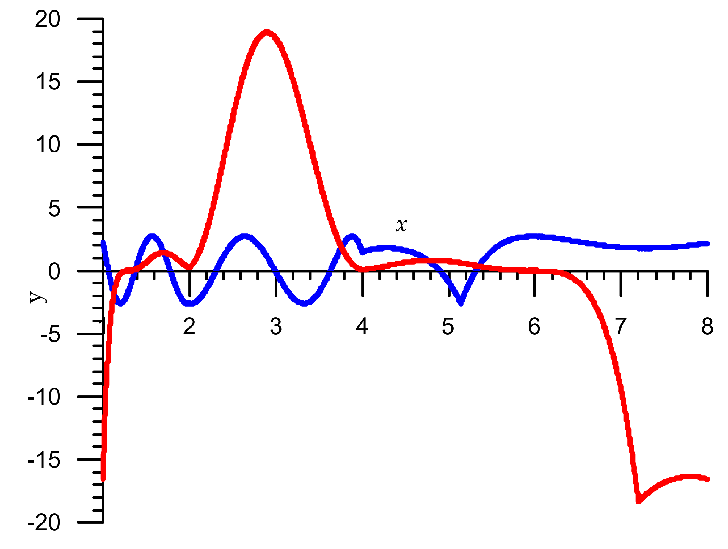
Figure 5 shows compatible graphs of relative errors for Algorithm 4 (red) and Algorithm 5 (blue) algorithms after the first iteration, where error = y·10−5. From analysis of Figure 5, it follows that in the Algorithm 5 there was a significant reduction in errors in the first iteration (7 times). This results in second iteration improvement (1.5 times). Note that the maximum relative errors of the Algorithm 5 for the first iteration are:
= 2.686·10−5 or = 15.18 correct bits.
Maximum relative errors for the second iteration are:
= 1.3301·10−7 or = 22.84 correct bits [1].
In order to calculate the cube root (Algorithm 6), the last lines of the algorithm codes related to the second iteration (for example, Algorithm 5, as well as any of the above algorithms).
| Algorithm 6. |
| 1: c = 1.0f − x*y*y*y; |
| 2: y = y*(1.0f + 0.333333333333f*c);//fmaf |
| 3: return y; |
| 4: should be written as follows: |
| 5: float d = x*y*y; |
| 6: c = 1.0f − d*y;//fmaf |
| 7: y = d*(1.0f + 0.333333333333f*c);//fmaf |
| 8: return y; |
4. Evaluation of Speed and Accuracy for Different Types of Microcontrollers
We researched the relative error of the aforementioned algorithms using a STM32F767ZIT6 microcontroller (manufacturer: STMicroelectronics) [22]. We determined the maximum negative and positive errors of two iterations for different algorithms (Table 1). These errors were calculated according to the formula InvCbrtK(x)*pow((double)x,1./3.)-1. for all numbers floating between [1,8], where K {1, 10, 11, 20, 21}. The maximum error was determined by the formula . Analysing the results of Table 1, we can see that Algorithm 5 gives the most accurate results in both iterations. In the last column, we present the results of errors which give the standard library function 1.f/cbrtf(). According to the results (Table 1) our Algorithm 5 (1.3301·10−7) has more than twice less error than the error of the library function (2.7947·10−7).
In addition, the operating time of the algorithm was researched. Testing was performed on four 32-bit microcontrollers with FPU.
- TM4C123GH6PM (manufacturer: Texas Instruments Incorporated, Austin, TX, USA)—microcontroller with 80 MHz tact frequency; compilers used were arm-none-eabi-gcc and arm-none-eabi-g++ (version 8.3.1).
- STM32L432KC (manufacturer: STMicroelectronics, Geneva Switzerland)—microcontroller with 80 MHz tact frequency; compilers used were arm-none-eabi-gcc and arm-none-eabi-g++ (version 9.2.1).
- STM32F767ZIT6 (manufacturer: STMicroelectronics)—microcontroller with 216 MHz tact frequency; compilers used were arm-none-eabi-gcc and arm-none-eabi-g++ (version 9.2.1).
- ESP32-D0WDQ6 (manufacturer: Espressif Systems, Shanghai, China)—microcontroller with 240 MHz tact frequency; compilers used were xtensa-esp32-elf-gcc and xtensa-esp32-elf-g++ [23].
We used two types of optimization for the -Os (smallest) and -O3 (fastest) microcontroller compilers. In all cases, the best optimization result was for -O3; therefore, we do not cite the optimization results of -Os.
Table 2 shows average function calculation times of InvCbrt(x) for Iteration I, which corresponds to 10,000,000 tests. Analysis of the results shows that the shortest calculation time is for the Algorithm 3 for all types of microcontrollers. Similar results are shown in Table 3 for Iteration II. In this table, we have added one more column with the results of the library function 1.f/cbrtf(). For the first three microcontrollers, the gain of the Algorithm 5 function is more than twice that of the library function and nine times better in terms of work gain for the microcontroller ESP32-D0WDQ6.
If we compare microcontrollers, we can see that the STM32F767ZIT6 is the fastest. Table 4 shows the results of algorithm performance on different microcontrollers for Iteration I, which is defined as the product of time calculating the inverse cube root and the tact frequency of the microcontroller (cycles).
Table 5 shows the results for Iteration II. In this table, we also have added one more column for library function 1.f/cbtf(). According to this table, the productivity of the function Algorithm 5 is twice better than the library function. Regarding microcontroller ESP32-D0WDQ6, the function Algorithm 5 works nine times better than the library function.
5. Conclusions
This paper presents results of a systematic analytical approach to the problem of increasing the accuracy of the inverse cube root code (including the optimal choice of magic constants). These provide minimum values of relative error for initial approximations according to the Newton–Raphson formula when calculating the function for float numbers. The optimal values of displacements for additive correction of Newton–Raphson formulas are also determined. These make it possible to reduce the relative errors of calculations. Thus, comparing the algorithms Algorithm 1 and Algorithm 2, the gain on the first iteration is approximately 1.97 times, and six times on the second iteration. The values of the coefficients of the Householder formula (order 2) were also optimized, making it possible to increase the calculation accuracy seven times (after the first iteration) without complicating the algorithm. In summary, we can conclude that the STM32F767ZIT6 microcontroller with -O3 optimization showed the best performance, and the Algorithm 3 was the fastest. Comparing the Algorithm 5 with the library function for microcontrollers, we can see that our algorithm is not only twice as accurate, but it can also calculate the function more than twice as fast (). These algorithms can also be implemented on an Intel Cyclone 10 GX (C10GX51001) FPGA [24].
In addition, the proposed algorithm can also be used to calculate the cubic root and can be implemented on Intel FPGA devices as it done in [25].
Author Contributions
Conceptualization, L.M.; Formal analysis, V.S.; Investigation, C.J.W. and L.M.; Methodology, V.S. and L.M.; Visualization, V.S.; Software, C.J.W.; Writing—original draft, J.L.C. and V.S.; Writing—review and editing, J.L.C. and V.S. All authors have read and agreed to the published version of the manuscript.
Funding
This research received no external funding.
Institutional Review Board Statement
Not applicable.
Informed Consent Statement
Not applicable.
Data Availability Statement
Data is contained within the article.
Conflicts of Interest
The authors declare no conflict of interest.
References
- Beebe, N.H.F. The Mathematical-Function Computation Handbook: Programming Using the Math. CWPortable Software Library; Springer: Berlin/Heidelberg, Germany, 2017. [Google Scholar]
- Moroz, L.; Samotyy, V. Efficient floating-point division for digital signal processing application [Tips and Tricks]. IEEE Signal. Process. Mag. 2019, 36, 159–163. [Google Scholar] [CrossRef]
- McEniry, C. The Mathematics Behind the Fast Inverse Square Root Function Code. Tech. Rep. August 2007. Available online: https://web.archive.org/web/20150511044204/http://www.daxia.com/bibis/upload/406Fast_Inverse_Square_Root.pdf (accessed on 14 February 2021).
- Moroz, L.; Walczyk, C.; Hrynchyshyn, A.; Holimath, V.; Cieslinski, J. Fast calculation of inverse square root with the use of magic constant—Analytical approach. Appl. Math. Comput. 2018, 316, 245–255. [Google Scholar] [CrossRef] [Green Version]
- Kahan, W. Computing a Real Cube Root. November 18, 1991. Available online: https://csclub.uwaterloo.ca/~pbarfuss/qbrt.pdf (accessed on 14 February 2021).
- Levin, S.A. Two point raytracing for reflection off a 3D plane. In Stanford Exploration Project; Citeseer: Princeton, NJ, USA, 2012; p. 89. Available online: http://sepwww.stanford.edu/data/media/public/oldsep/stew/ForDaveHale/sep148stew1.pdf (accessed on 14 February 2021).
- Guardia, C.M.; Boemo, E. FPGA implementation of a binary32 floating point cube root. In Proceedings of the IX Southern Conference on Programmable Logic. (SPL), Buenos Aires, Argentina, 5–7 November 2014. [Google Scholar] [CrossRef]
- Pineiro, A.; Bruguera, J.D.; Lamberti, F.; Montuschi, P. A radix-2 digit-by-digit architecture for cube root. IEEE Trans. Comput. 2008, 57, 562–566. [Google Scholar] [CrossRef]
- Shelburne, B.J. Another method for extracting cube roots. In Stanford Exploration Project; Department of Mathematical and Computer Science, Wittenberg University: Springfield, OH, USA, 2012; Available online: http://citeseerx.ist.psu.edu/viewdoc/download?doi=10.1.1.99.7241&rep=rep1&type=pdf (accessed on 14 February 2021).
- Moroz, L.; Samotyy, V.; Horyachyy, O.; Dzelendzyak, U. Algorithms for calculating the square root and inverse square root based on the second-order Householder’s method. In Proceedings of the 2019 10th IEEE International Conference on Intelligent Data Acquisition and Advanced Computing Systems: Technology and Applications (IDAACS), Metz, France, 18–21 September 2019; pp. 436–442. [Google Scholar] [CrossRef]
- Szanto, G. 64-bit ARM Optimization for Audio Signal Processing; Superpowered: Austin, TX, USA, 2019; Available online: https://superpowered.com/64-bit-arm-optimization-audio-signal-processing (accessed on 14 February 2021).
- Xilinx Forums. How to Accelerate the Floating Point Implementation for Cube Root on VU9P. October 08, 2019. Available online: https://forums.xilinx.com/t5/AI-Engine-DSP-IP-and-Tools/How-to-accelerate-the-floating-point-implementation-for-cubic/td-p/1034998 (accessed on 14 February 2021).
- DSP Related.Com. Fast Cube Root Using C33. February 26, 2009. Available online: https://www.dsprelated.com/showthread/comp.dsp/109311-1.php (accessed on 14 February 2021).
- Short Vector Math Library (SVML). September 25, 2018. Available online: https://community.intel.com/t5/Intel-C-Compiler/Short-Vector-Math-Library/td-p/857718 (accessed on 14 February 2021).
- Integrated Performance Primitives (IPP). Available online: https://software.intel.com/content/www/us/en/develop/tools/integrated-performance-primitives.html (accessed on 14 February 2021).
- Fog, A. Software Optimization Resources, Instruction Tables: Lists of Instruction Latencies, Throughputs and Micro-Operation Breakdowns for Intel, AMD and VIA CPUs. January 31, 2021. Available online: https://www.agner.org/optimize/instruction_tables.pdf (accessed on 14 February 2021).
- Turkowski, K. Computing the Cube Root. Apple Computer Technical Report No. #KT-32; February 10, 1998. Available online: https://people.freebsd.org/~lstewart/references/apple_tr_kt32_cuberoot.pdf (accessed on 14 February 2021).
- Cpluspus.com. Available online: http://www.cplusplus.com/reference/cmath/cbrt/ (accessed on 14 February 2021).
- Muller, J.-M. Elementary functions and approximate computing. In Proceedings of the IEEE (Early Access); IEEE: Piscataway, NJ, USA, 2020; pp. 1–14. [Google Scholar] [CrossRef]
- Walczyk, C.J.; Moroz, L.V.; Cieśliński, J.L. A modification of the fast inverse square root algorithm. Computation 2019, 7, 41. [Google Scholar] [CrossRef] [Green Version]
- Walczyk, C.J.; Moroz, L.V.; Cieśliński, J.L. Improving the accuracy of the fast inverse square root algorithm. Entropy 2021, 23, 86. [Google Scholar] [CrossRef] [PubMed]
- STmicroelectronics. Ultra-low-power with FPU Arm Cortex-M4 MCU 80 MHz with 256 Kbytes of Flash Memory, USB. Available online: https://www.st.com/en/microcontrollers-microprocessors/stm32l432kc.html (accessed on 14 February 2021).
- EspressifSystems. ESP32-WROOM-32 (ESP-WROOM-32) Datasheet; Version 2.4; Espressif Systems: Shanghai, China, 2018; Available online: https://www.mouser.com/datasheet/2/891/esp-wroom-32_datasheet_en-1223836.pdf (accessed on 14 February 2021).
- Intel. Intel Cyclone 10 GX Device Overview: C10GX51001. January 4, 2019. Available online: https://www.intel.com/content/www/us/en/programmable/documentation/grc1488182989852.html (accessed on 14 February 2021).
- Faerber, C. Acceleration of Cherenkov angle reconstruction with the new Intel Xeon/FPGA compute platform for the particle identification in the LHCb Upgrade. J. Phys. Conf. Ser. 2017, 898. [Google Scholar] [CrossRef] [Green Version]
Figure 1.
The first iteration relative error graphs for the interval x ∈ [1,8) (red color: Algorithm 1, blue color: Algorithm 2).
Figure 1.
The first iteration relative error graphs for the interval x ∈ [1,8) (red color: Algorithm 1, blue color: Algorithm 2).
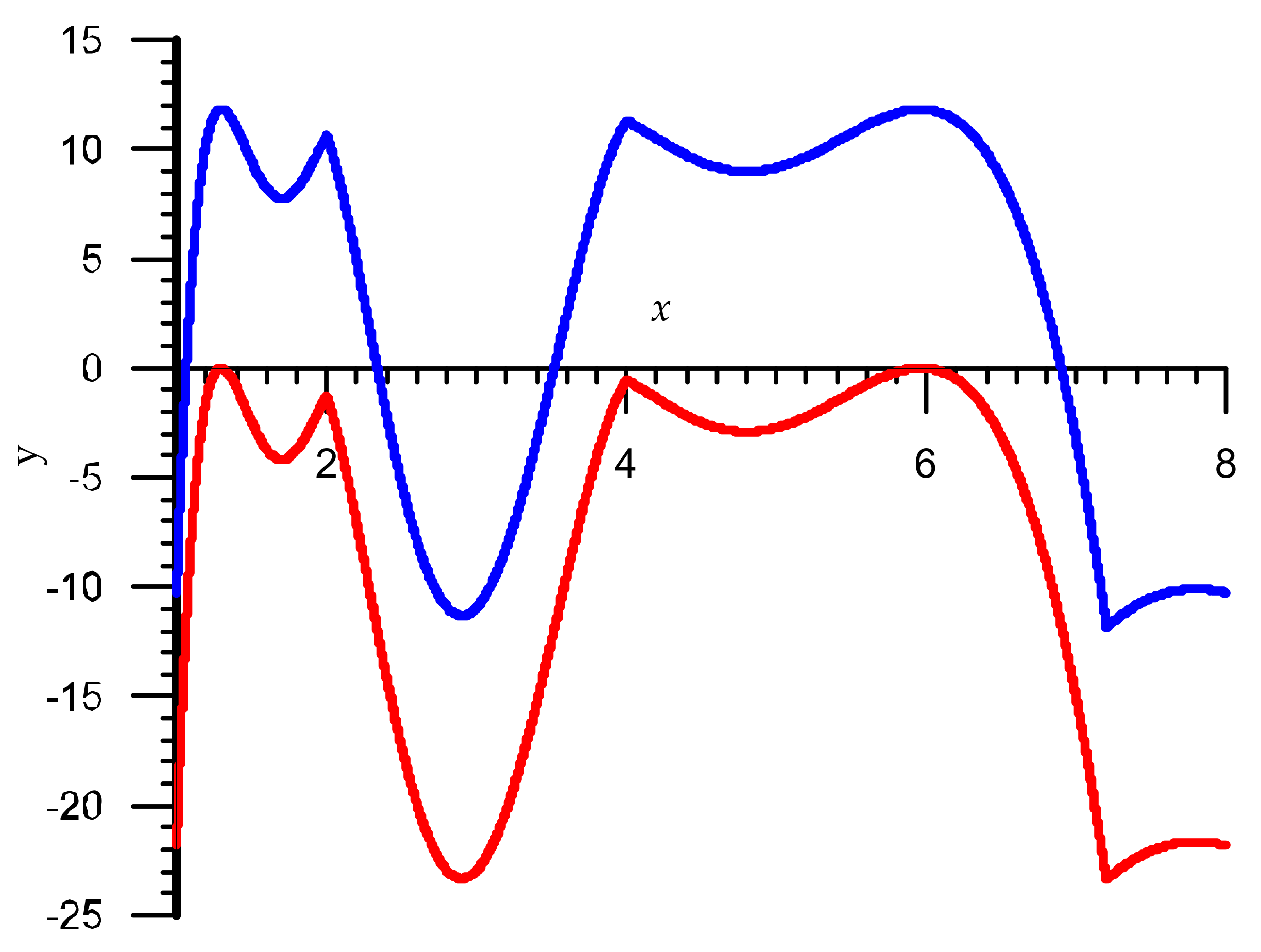
Figure 2.
The first iteration relative error graphs Algorithm 3 for the interval x ∈ [1,8).
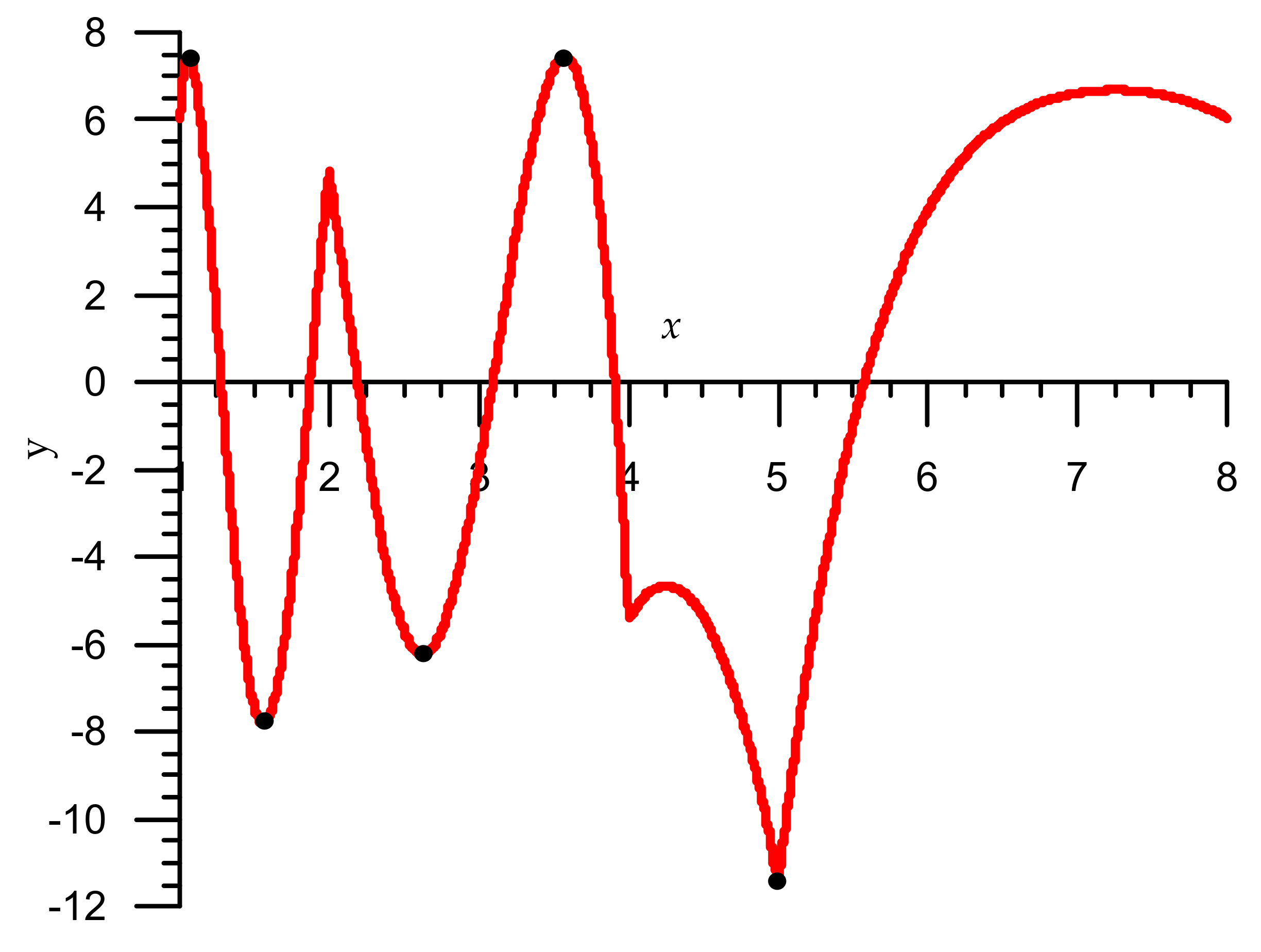
Figure 3.
The first iteration relative error graphs Algorithm 3 for the interval x ∈ [1,8).
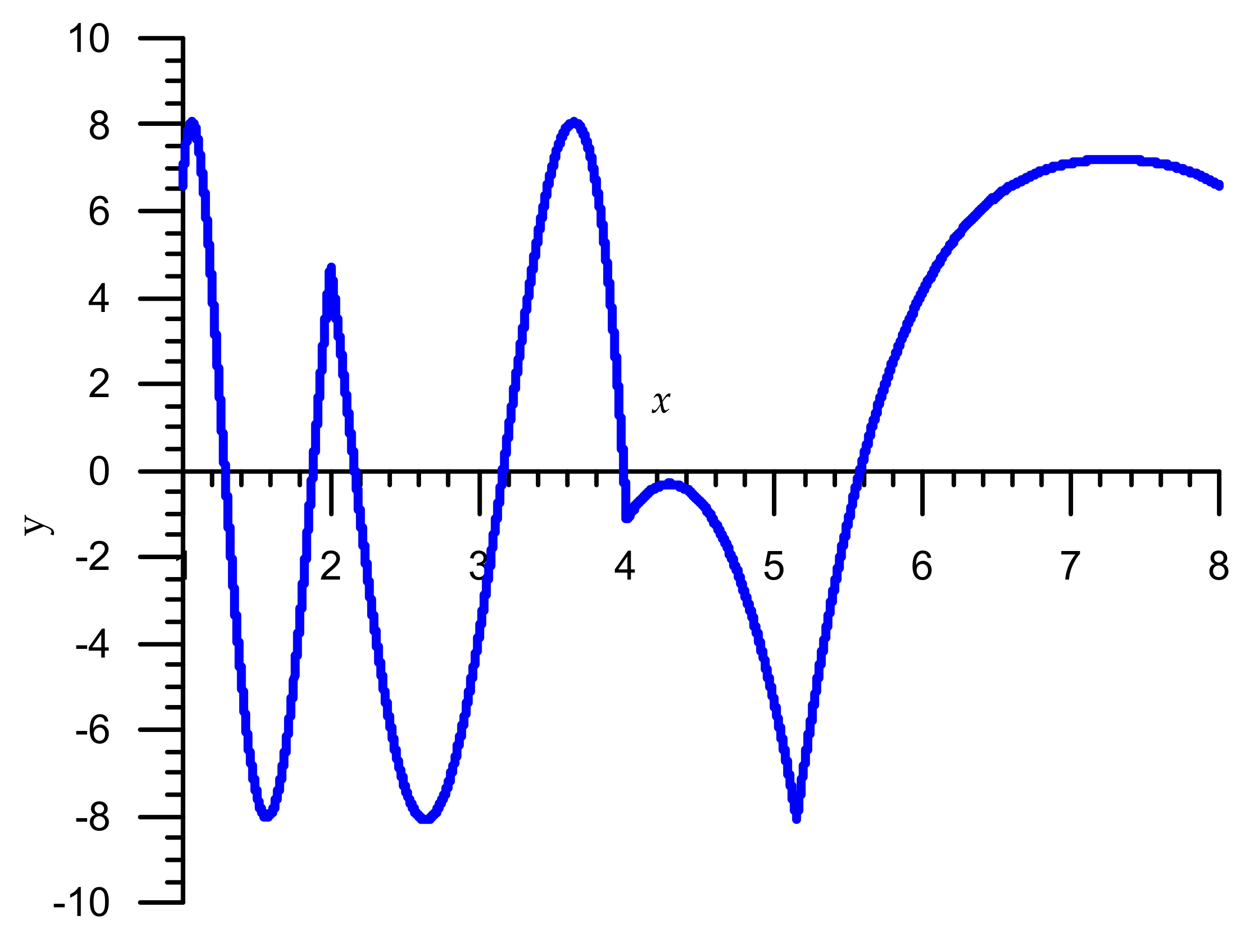
Figure 4.
The first iteration relative error graphs Algorithm 5 for the interval x ∈ [1,8).
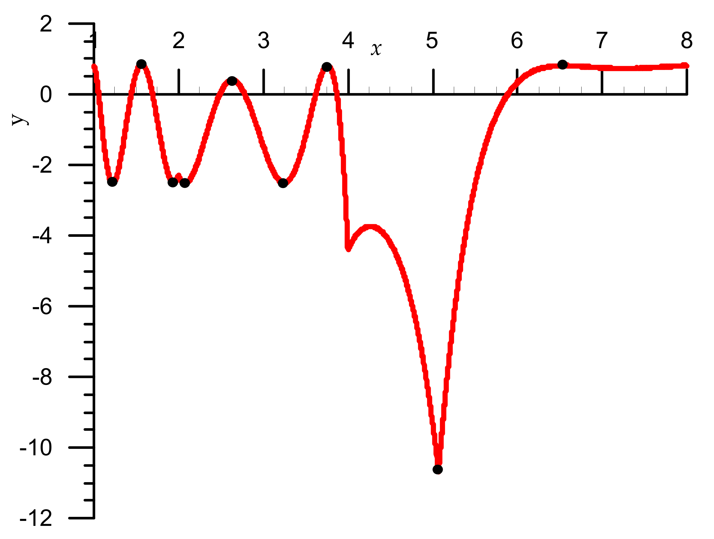
Figure 5.
The first iteration relative error graphs for the interval x ∈ [1,8) (red colour: Algorithm 4, blue colour: Algorithm 5).
Figure 5.
The first iteration relative error graphs for the interval x ∈ [1,8) (red colour: Algorithm 4, blue colour: Algorithm 5).

Table 1.
The maximum negative and positive errors of two iterations for different algorithms.
| Iteration I | Iteration II | |||
|---|---|---|---|---|
| Algorithm | ||||
| 1 | −2.3386·10−3 | 1.7063·10−7 | −1.1032·10−5 | 1.8301·10−7 |
| 2 | −1.1826·10−3 | 1.1828·10−3 | −1.8355·10−6 | 1.2510·10−6 |
| 3 | −8.0837·10−4 | 8.0523·10−4 | −8.0803·10−7 | 7.6980·10−7 |
| 4 | −1.8350·10−4 | 1.8922·10−4 | −2.0021·10−7 | 1.3298·10−7 |
| 5 | −2.6860·10−5 | 2.6825·10−5 | −1.3276·10−7 | 1.3301·10−7 |
| 1.f/cbrtf() | - | - | −2.6004·10−7 | 2.7947·10−7 |
Table 2.
Average function calculation times of InvCbrt(x) for Iteration I.
| Iteration I with Optimization -O3 | ||||||
|---|---|---|---|---|---|---|
| Microcontroller | ||||||
| 1 | TM4C123GH6PM | 625.91 | 650.95 | 625.91 | 726.06 | 701.01 |
| 2 | STM32L432KC | 487.85 | 487.85 | 475.34 | 575.41 | 562.9 |
| 3 | STM32F767ZIT6 | 166.7 | 166.7 | 162.07 | 203.75 | 199.12 |
| 4 | ESP32-D0WDQ6 | 239.27 | 239.27 | 239.27 | 264.48 | 264.48 |
Table 3.
Average function calculation times of InvCbrt(x) and fl() = 1.f/cbrtf() for Iteration II.
| Iteration II with Optimization -O3 | |||||||
|---|---|---|---|---|---|---|---|
| Microcontroller | fl()[ns] | ||||||
| 1 | TM4C123GH6PM | 776.13 | 776.13 | 826.21 | 976.42 | 976.44 | 1953 |
| 2 | STM32L432KC | 612.93 | 637.95 | 650.46 | 763.05 | 763.05 | 1588 |
| 3 | STM32F767ZIT6 | 231.54 | 231.54 | 226.91 | 291.74 | 287.11 | 625 |
| 4 | ESP32-D0WDQ6 | 310.65 | 306.47 | 306.46 | 377.82 | 377.82 | 3479 |
Table 4.
The results of algorithm performance on different microcontrollers for Iteration I.
| Iteration I with Optimization -O3 | |||||||
|---|---|---|---|---|---|---|---|
| Microcontroller | [MHz] | ||||||
| 1 | TM4C123GH6PM | 80 | 50.1 | 52.1 | 50.1 | 58.1 | 56.1 |
| 2 | STM32L432KC | 80 | 39.0 | 39.0 | 38.0 | 46.0 | 45.0 |
| 3 | STM32F767ZIT6 | 216 | 36.0 | 36.0 | 35.0 | 44.0 | 43.0 |
| 4 | ESP32-D0WDQ6 | 240 | 57.4 | 57.4 | 57.4 | 63.5 | 63.5 |
Table 5.
The results of algorithm performance on different microcontrollers for Iteration II.
| Iteration II with Optimization -O3 | ||||||||
|---|---|---|---|---|---|---|---|---|
| Microcontroller | [MHz] | 1.f/cbrtf() | ||||||
| 1 | TM4C123GH6PM | 80 | 62.1 | 62.1 | 66.1 | 78.1 | 78.1 | 156 |
| 2 | STM32L432KC | 80 | 49.0 | 51.0 | 52.0 | 61.0 | 61.0 | 127 |
| 3 | STM32F767ZIT6 | 216 | 50.0 | 50.0 | 49.0 | 63.0 | 62.0 | 135 |
| 4 | ESP32-D0WDQ6 | 240 | 74.6 | 73.6 | 73.6 | 90.7 | 90.7 | 835 |
Publisher’s Note: MDPI stays neutral with regard to jurisdictional claims in published maps and institutional affiliations. |
© 2021 by the authors. Licensee MDPI, Basel, Switzerland. This article is an open access article distributed under the terms and conditions of the Creative Commons Attribution (CC BY) license (http://creativecommons.org/licenses/by/4.0/).
Share and Cite
MDPI and ACS Style
Moroz, L.; Samotyy, V.; Walczyk, C.J.; Cieśliński, J.L. Fast Calculation of Cube and Inverse Cube Roots Using a Magic Constant and Its Implementation on Microcontrollers. Energies 2021, 14, 1058. https://doi.org/10.3390/en14041058
AMA Style
Moroz L, Samotyy V, Walczyk CJ, Cieśliński JL. Fast Calculation of Cube and Inverse Cube Roots Using a Magic Constant and Its Implementation on Microcontrollers. Energies. 2021; 14(4):1058. https://doi.org/10.3390/en14041058
Chicago/Turabian StyleMoroz, Leonid, Volodymyr Samotyy, Cezary J. Walczyk, and Jan L. Cieśliński. 2021. "Fast Calculation of Cube and Inverse Cube Roots Using a Magic Constant and Its Implementation on Microcontrollers" Energies 14, no. 4: 1058. https://doi.org/10.3390/en14041058
Note that from the first issue of 2016, this journal uses article numbers instead of page numbers. See further details here.