Abstract
The energy transition in Germany takes part in decentral structures. With the ongoing integration of Renewable Energy Sources (RES) into the electricity supply system, supply-side is therefore becoming increasingly decentral and volatile due to the specific generation characteristics. A rather inflexible demand-side, on the other hand, increases the effort to gain the necessary equilibrium between generation and consumption. This paper discusses how consumer behaviour can be influenced by real-time pricing to align demand with generation. Therefore, a combination of two different approaches is used, (I) The Cellular Approach (CA) and (II) Agent Based Modelling (ABM). A model is set up considering a regional energy market, where regional electricity products can be traded peer-to-peer regarding each consumer’s preferences. The observation is made for a whole distribution grid including all types of consumers. The investigations show that energy purchases can be stimulated individually by a flexible pricing mechanism and met preferences. Moreover, benefits occur for the whole region and potentials arise to smooth the exchange balance to the superordinate grid level. Running the model for one entire year in a conservative generation scenario, hours of oversupply could be reduced by and the consumption of green electricity generated regionally could be increased by over within the region itself, in comparison to a base scenario.
1. Introduction
A stable electricity system is highly dependent on a permanent equilibrium between generation and consumption. Therefore, flexibility of both sides is a fundamental need. Up to now, this flexibility is mainly provided through the supply-side factors [1]. However, while the German energy transition progresses, volatility and decentralism become permanent supply-side characteristics. In contrast to this, demand-side will not change to this extent and consumption remains rather inflexible in spatial as well as in temporal sense. Consequently, the organisational effort for gaining the equilibrium increases tremendously [2,3].
To secure the supply throughout the whole energy system it is no longer sufficient to regulate only the supply-side. Supply and demand have to be managed and adjusted mutually. Because of the increasing shares of decentral generation units primarily based on RES there is a rising potential for enhanced interconnections of generation and consumption on local grid levels. Therefore, it is indispensable to create more flexibility on the demand-side [4]. However, it is still not answered satisfactorily yet, how to change or influence consumer behaviour effectively.
As generation out of RES is highly weather dependent there is no way of influencing its temporal amount manually [5]. Various technical solutions, e.g., battery storages or power-to-x-technologies, enable the temporal decoupling of generation and consumption to a certain extent. Another approach, the so-called demand side management, follows the idea of shifting or cutting load peaks to meet the amount of generation [4,5]. These and other technical aids will be one part of the overall solution for reaching Germany’s climate goals. The other part of the solution will be the consumer itself [6].
In supply systems with increasing shares of RES, the former classification between consumers and producers tends to be blurred. In other words, consumers become partly producers, so-called “prosumers”, or at least shareholders of generation units [7,8]. Since electricity is a homogeneous commodity in the physical sense, some consumer groups make distinctions regarding the energy source. For example, electricity from the rooftop photovoltaic (PV) system is preferred compared to electricity from the public grid. Furthermore, the location of generation is important to some consumers [9].
With regard to this, the question of possible impacts on regional supply and demand arises. Therefore an agent-based model is created to analyse counterfactual scenarios, by taking into account the constraining boundaries of a real existing local supply system, where all consumer groups (Households; Trade, Commerce and Services; Industry) are simulated as full-fledged equal market participants in a regional energy market. This market is not understood as a self-sufficient isolated market, but rather as an integrated unit in an interregional wholesale energy market. Moreover, this approach does not attempt to achieve a cost optimization of the total system by means of idealized equilibrium models, but to investigate the impacts of consumer behaviour from a bottom-up perspective.
2. Background and Literature
As the German energy transition progresses, the number of renewable, near-load electricity generation units will increase and by this, the amount of electricity fed into the distribution grid level [10]. If the electricity cannot be consumed locally, it will be transferred to the upper grid levels and transported to other regions where generation does not exceed the demand. This trend will inevitably continue to grow in the course of the energy transition [11].
A prerequisite for this interregional electricity exchange is sufficient grid capacity. However, since the grid is not actually a copper plate, bottlenecks may occur. To avoid bottlenecks (I) grid expansion and (II) redispatch of generation units are inevitable. (I) On the one hand, grid expansion is in many cases the most cost-effective flexibility option, i.e., the costs of regional equilibration may exceed the costs of additional grid expansion. On the other hand, designing the grid for the so-called last kilowatt-hour is not economically efficient [10,12]. (II) Costs for redispatch in Germany increased continuously in the last decade [13].
Against this background, the question arises to which extend the trading of green and regional electricity can contribute to the success of the energy transition and the development of supply systems. Currently there is neither a solid business model nor a suitable regulatory framework for the trading of green and regional electricity. So, no prerequisites for a continuous market development are given. Until now, there is a lack of systematic understanding of the added value of regional green power marketing in terms of both the energy industry and society [10].
Lueth et al. (2020) [14] tested recently proposed regional market designs under the current rules in the context of the German market. All presented concepts were financially unattractive to prosumers and consumers within the current regulatory framework.
On the other hand, the systematized review of [15] on different time of use electricity tariffs shows that there definitely exists demand for flexible price tariffs. Moreover, refs. [16,17] show that price signals can trigger a reaction and adjustment in electricity demand of different consumer groups and further that there is an impact on the market.
Mainzer (2018) [18] points, that there is a significant potential for covering the energy demand on the basis of renewable energies, especially in smaller communities. Mainzer (2018) [18] also shows that the transformation of the urban energy system towards the use of local and sustainable energy resources can be the preferred alternative. But as [18,19] primarily inspect the issue out of the systems perspective using top-down equilibrium models, this paper’s model focuses primarily on the consumer groups itself.
Pokropp (2012) [20] analyses environmentally conscious decisions regarding the purchase of green electricity by residential costumers and focuses on the consumer’s preferences. This paper uptakes this approach, extends it to the preference for regionality and adopts it not only for one specific but for all consumer groups within the supply system.
As already mentioned there is no regulatory framework for the regional trading of green and regional electricity. The basic idea to design this paper’s market model was to create a tool which enables to discuss different pathways and regulatory frameworks on how to foster local consumption of regionally generated electricity throughout various generation and demand scenarios regarding different population and industrial structures.
3. Methodology and Materials
3.1. Methodology
3.1.1. Cellular Approach
Future electricity supply systems reach for environmental sustainability on a high level and thus integrating high shares of fluctuating RES. With regard to the challenge of adjusting supply and demand mutually, this requires new approaches with an increased degree of system control.
The so-called “Cellular Approach” is such an approach. The CA offers a broad range of potential benefits for integrating RES in local distribution grids, while always balancing supply and demand on the lowest possible level. Therefore, the CA is based on energy cells. Cells are characterized by their ability to generate, consume, and store energy. Every cell can connect to other cells and, thereby, build superordinate energy cells in turn (see Figure 1). Moreover, each cell aims to equilibrate generation and consumption by itself. If the equilibrium cannot be reached alone, the cell connects to other cells to reach it.
To rephrase this and give an example, imagine a private household operating a PV system. This household is the lowest possible cell, always trying to fit its electricity consumption to its generation or vice versa. In case of higher supply than demand, this household connects to other cells in the system, maybe to another household, and sells its leftover electricity. Or in contrast, buys electricity from other cells if demand is higher than supply.
In [21] the technical feasibility of the CA is approved. The logic of the CA also allows the outlined marketing concept above. By this, security of supply and economic efficiency can be ensured. Furthermore, public acceptance regarding the transformation of the supply system can be enhanced, since consumers have the opportunity to participate at the market.

Figure 1.
Energy cells (Authors own compilation based on [22]).
Figure 1.
Energy cells (Authors own compilation based on [22]).

3.1.2. Agent Based Modelling
As mentioned in Section 1, this work’s focus is not on minimizing the costs of the overall system by use of perfect foresight equilibrium models, but rather on simulating consumer behaviour and investigating possible impacts on the supply system. Consequently, ABM is the method of choice.
ABM allows the simulation of imperfect markets and competition. Therefore, agents represent various market participants acting with strategic behaviour based on asymmetrical information. Moreover, learning effects due to repeated interactions can be modelled as well [23,24,25,26]. Furthermore, ABM enables to investigate several system levels in different degrees of abstraction. Especially the interdependency between the microscopic level, where agents act, and the macroscopic level, where system behaviour emerges, can be observed [27].
In combination with the CA, a model is set up to observe emerging consumer behaviour in a counterfactual energy market scenario. Each agent represents one market participant acting by its own preferences. Thereby each market participant represents one low-level energy cell trying to equilibrate its generation and consumption by changing behaviour or connect to the other energy cells.
4. The Model
4.1. Basics
This simulation model, the so-called Regional Energy Market Model (REMM), is built in NetLogo (see Appendix C.1) as a bottom-up approach for integral load management and is designed to investigate decentralised energy markets. So far modelled for short-term scenarios, the observation period covers one year in a one-hour resolution beginning from January 1st.
The observed electricity system is defined as a local distribution grid with its typical producing and consuming entities, covering an area of 100 km partitioned as a predefined 10 by 10 mesh with 100 patches each of 1 km (see Appendix C.2). In order to reflect generation from RES properly, a database is linked to the model providing true local weather data for wind speed, solar radiation, and temperature. The data is obtained by the Test Reference Years (TRY) of the German Meteorological Service (DWD, see Appendix C.1 and Appendix C.2).
In general, the model can display and simulate various supply and demand scenarios with specific characteristics. For now, an exemplary scenario was set up, which is comparable to the supply system of Zittau, a town in East Germany with 26,500 inhabitants. Zittau has its own local utility company (LUC) and grid, which perfectly fits to the purpose of the model. Once set up to supply higher amounts of consumers, the local grid is slightly oversized so that no grid constraints exist in the model.
Figure 2 gives an overview over the REMM and its entities.
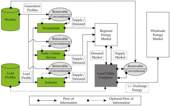
Figure 2.
Overview model structure.
4.2. Demand-Side
The following three representative consumer groups are integrated in the REMM:
- Private Households-model name: Residential with Standard Load Profile (RSL)
- Trade, Commerce, and Service-model name: Business with Standard Load Profile (BSL)
- Industry-model name: Business with Measured Load Profile (BML).
The consumption of RSL agents is characterised by the (dynamic) standard load profile H0. Standard load profiles for Germany were published by the German Electricity Association (VDEW, see Appendix C.1). Furthermore, BSL agents are characterised by the standard load profile G0. These profiles are standardised to an annual consumption of 1000 kWh and have to be scaled up to use them in the model. Therefore, each hourly value of the profiles is multiplied by a coefficient randomly chosen out of a given domain (see Table 1) and assigned to each of these agents before the simulation starts. In practice, local utilities use the annual consumption of the prior year to determine the scale factor for the present year. However, the REMM observes only one year, so that it has to predefine this coefficient itself. Nevertheless, this complies with the approach most of the local utilities use to forecast the annual consumption of standard load profile consumers. Find further information on these scale factors in Appendix A.

Table 1.
Scale factor domains for load profiles.
For BML agents no standard load profiles exist. Therefore, empirical load profiles were created, which were derived from actually measured profiles of several real existing companies, which are comparable to those companies typically connected to the distribution grid. By this, three load profiles were generated representing different types of companies distinguished by their annual electricity consumption (see Table 2).
Table 2.
Types of artificial load profiles for BML agents.
The allocation of scale factors to every agent is primarily a random decision by the REMM. Nevertheless, constraints ensure that the model depicts the overall picture of the average distribution of household or business sizes in Germany and by this their overall electricity consumption [28,29,30,31] (see also Appendix A). The localisation of RSL, BSL and BML agents across the model’s area is comparable to the real conditions of Zittau’s supply system. In total, the REMM comprises 15,407 RSL, 1638 BSL and 108 BML agents.
All these entities are consciously modelled out of the systems perspective. That means, they are mainly characterised by two attributes, consumption and demand . While consumption describes the total electricity need of an agent i per time step t, demand describes his hourly electricity purchase from the grid. For most of the agents applies . However, some agents (prosumer) are able to partially generate their own electricity, so that their demand is smaller than their consumption (see Section 4.3).
4.3. Supply-Side
The supply-side is also modelled out of the systems perspective, primarily focusing on the agent’s generation patterns. To model generation characteristics properly, several possibilities of decentral electricity generation are implemented in the model (see Table 3). To represent the volatile feed-in through RES, PV systems are implemented. Controllable renewable and controllable conventional generation characteristics are integrated via combined heat and power (CHP) units, which are operated either with biogas or natural gas. Via the model’s interface, the total amount of generation units and, thereby, the possible capacity in the REMM can be predefined by the user.
Table 3.
Implemented generation units.
All units are operated by demand-side agents of the model. Which agents becomes a so-called prosumer is a random decision by the model. Every prosumer can possess a PV rooftop unit and/or a combined heat and power (CHP) unit (see Table 3). The generation capacity of these units is aligned to the annual electricity consumption of the operating agent. Generation out of PV is captured via standardised rooftop modules (see Appendix B). For reasons of practicability, a constraint is embedded that PV systems may not be smaller than 3 kW. Furthermore, the model is only allowed to raise power capacities by steps of 250 W. The CHP capacity of an agent results out of his annual electricity consumption and the expected full load hours of 6000 h p.a. (see Appendix B). Constraints allow the model to only adjust the CHP capacity to the agent’s consumption pattern in steps of 500 W. CHP plants in the REMM are operated in a heat-controlled mode. Therefore, the daily average temperatures were determined based on the exogenous weather data. If the average temperature of the following day falls below the heating limit given in the model’s interface (C), the CHP system is switched on for the next full 24 h and operates on nominal load. On the one hand, this assumption is made on the storage effect of the buildings mass and, further, on the most probable fact that heating facilities based on CHP are built in combination with buffer storages.
Each prosumer prefers to consume its self-generated electricity to cover his consumption. In times where generation is greater than consumption, prosumers sell their leftover electricity at the regional market. If generation is lower than consumption, prosumers will buy the missing electricity at the market (see Equation (1)).
4.4. Local Utility Company
The LUC, with its own generation possibilities and its connection to the wholesale market, represents central fluctuating RES and central controllable conventional energy sources.
As there is a local market and a local supply system, there consequently has to be a system operator who ensures the equilibrium between generation and consumption at any time. In REMM, this is the LUCs responsibility. Due to the fact that the model’s observations are all about the behaviour of the consumers, the LUC is modelled as a passive agent. Passive means that the LUC acts without any intention of making profit as the enabler, maintaining the overall system and reading the market to meet the consumer’s demand. Therefore, the utility has various options. One can be to use its own renewable as well as conventional generation facilities. Another is to sell or buy electricity from the interregional wholesale market depending on regional over- or undercapacities respectively.
4.5. Market Design and Pricing Mechanism
The simulation is carried out for a market trading four different electricity products. Figure 3 shows their modular configuration, based on three different price components. Key differentiators are the energy source, so whether the electricity comes from renewable or conventional sources, and the transmission distance, that means the distance between producer and consumer. By this mechanism, green and grey products are available at each market both with a regional or an interregional background. Taxes accrue for every product.
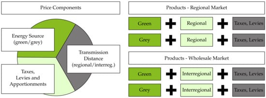
Figure 3.
Price components and electricity products.
As Figure 2 shows, consuming agents have only direct access to the regional market. However, that does not mean that they are only able to buy regional products. Interregional products are offered via the LUC, which is the connector between both markets. As mentioned, all prosumers are allowed to offer their self-generated electricity at the regional market, in case of overcapacities, as a regional product.
Energy Source. To keep the model simple, the simulation works with fixed prices for every time step. To rephrase this, neither the regional nor the interregional market owns a further pricing mechanism, like the merit-order approach. It’s the LUCs responsibility to set the prices. For purchasing the grey product, consumers only have to pay the base price , whereas for the green product, a price premium for green energy has to be paid additionally. This premium is comparable with the German Renewable Energies Act levy (EEG-Umlage). It can be seen as a promotion for renewable energy sources.
Transmission Distance. By choosing a regional or an interregional product, the consumer decides about the height of the grid fee. The larger the distance, the higher the fee. As mentioned above (see Section 4.1), the models world is a 10 by 10 mesh with 100 patches. All producers located on one of these patches, are considered as producers offering regional electricity. On the contrary, all electricity generated not within this area is considered as interregional. Of course, the grid fee for interregional electricity is different than for regional. Both can be predefined in the model’s interface.
Taxes, Levies and Apportionments. This is a fixed term depending on the consumer group each agent belongs to (see Section 4.2). For each group, the user can again predefine the actual value individually in the interface. To take into account that BSL and BML agents tend to be more energy-intensive than RSL agents are, it is recommended to make a quantity-dependent graduation. So that RSL consumers pay the highest taxes, in relative terms, followed by BSL consumers, while BML agents pay less. Note that as taxes are levied on every product, they provide no incentive and thus do not affect the consumer’s behaviour and their decision making (see Section 4.6).
4.6. Consumer Behaviour and Decision Making
Starting point for each agent’s decision is his environmental awareness, regional awareness and his budget (see Table 4). Environmental awareness describes his individual esteem for green energy sources. Regional awareness represents his preference for electricity generated in a local context. For both, a value close to one indicates a high preference, a value close to zero a low preference. Budget describes his individual assessment of higher costs. The budget is directly dependent on his income, in case of RSL, respectively on his earnings, in case of BSL or BML, and expresses in his preference for the price. A value close to one indicates a high sensitivity for costs, a value close to zero a low sensitivity, what would mean that these agents would pay higher prices.
Table 4.
Domains of consumer preferences.
Each time step, all consumers take a new decision which electricity product they preferably purchase. In general, this is a two stage decision process. Agents compare between the grey and green products respectively the regional and interregional products by calculating their values U. Finally, that product is chosen which promises the biggest personal value.
Analogous to the work of [20], the inertia of human decision making is captured in the REMM regarding two points. On the one hand the preference for the status quo is regarded. People tend to prefer easy and fast decision processes in their every day life, especially for commodities like electricity that are not visible or tangible for them. Consumers, especially RSL, do not assess these products continuously. There is a asymmetric assessment, preferring the own current status [20].
On the other hand the REMM takes delayed price perception, or in other words a lack of information in prices, into account. Pokropp (2012) [20] mentions, that consumers have a big lack of information regarding their annual electricity consumption and related costs. It is therefore not expected, that RSL agents or agents representing small companies, have a 100% overview of the market and prices.
Preference for the status quo. For switching from the initial to the alternative product, the benefit of the alternative utility value must be at least greater than the utility value of the initial product plus a certain threshold value . can be predefined in the models interface for each consumer group separately. Explained on the example of purchasing grey electricity this means:
Delayed price perception. Decisive for the utility value calculations are not the current values of the price components, but rather the perception agents have about these variables. With a time lag, perceptions will align to the current decision variables. Therefore, a differential adjustment process with the exogenous variable is implemented. can be predefined in the models interface for each consumer group separately. Perceptions of price components are written in calligraphic letters (see Table 5).
Table 5.
Formula symbols for perception.
Explained on the example of the perception of the base price this means:
Utility values of stage I. Similar to the approach in [20] the utility value U is calculated by each agent by comparing an intrinsic value with the negative value of (higher) costs . For the calculation of the intrinsic value it is estimated that one unit of the extra mark-up , respectively the perception , for renewable energies can be converted in exactly one unit of an abstract personal good, that can be interpreted as well-being or moral satisfaction. The intrinsic value results out of the agent’s environmental awareness e combined with its price sensitivity c and the amount of . By this, the intrinsic value for the purchase of grey electricity is 0.
This intrinsic value is compared with the (negative) effect of higher costs caused by the extra the mark-up for green electricity. The value results under consideration of each agent’s price sensitivity c and his perception of the price components and .
By combining and the overall utility functions for the purchase of green and grey electricity result as follows.
Utility values of stage II. Analogous to stage I the utility values U in stage II also result out of the comparison between the intrinsic values and the values of costs . It is furthermore assumed, that an intrinsic value only for the purchase of electricity generated in a regional context exists. The intrinsic value for interregional purchase is 0.
The utility value of costs results similar to the approach in stage I as follows.
Combining both, intrinsic value and value of costs, the overall utility functions for regional and interregional purchase appear es follows.
4.7. Market Clearing
Since CHPs only operate at low temperatures and PVs only generate electricity while the sun is shining, the regional market is highly volatile. Consequently, situations can arise where parts of the preference-driven demand cannot be met. It’s the LUC’s responsibility to clear the market. Situations characterised by a regional oversupply are not crucial for the simulation, because of the assumption that leftover electricity could be sold at the wholesale market at any time. However, situation with undersupply of both or at least one of the regional products are challenging, because a decision has to be made, who of the applying agents gets served and who has to switch to another product and on which decision base the switch happens. This second situation is shown in Figure 4.
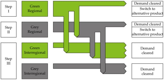
Figure 4.
Market clearing scheme and alternative products.
The decision who of the applying agents gets served is based on their willingness to pay (WTP). The WTP can be derived out of the utility functions U. By equating the Functions (8) and (9) and converting to , the amount of money can be calculated at which an agent would just about prefer the green product to the grey one. Analogous this works for the WTP for the regional product by equating the Functions (12) and (13) and converting to .
Step I. The first step is the clearing of the green regional market section. Therefore, all applying agents are listed on the basis of their WTP for green. Agents with high a WTP are served first, agents with a low WTP last.
Agents who cannot be served are forced to switch to an alternative product. Since the initial decision of these agents is based on both special predicates, green and regional, it is decisive in the choice of the alternative product, which of the two predicates the agent would most likely forego. Indicators for this decision are the individual preferences environmental awareness e and regional awareness l, which already provide a weighting. The agent therefore decides whether he wants to continue to be green but no longer regional or would like to remain regional but no longer buy green.
While clearing this market section the supply of green power decreases continuously with each agent served. It is highly unlikely that the remaining trading volume while serving the last possible agent will exactly match his demand. Usually the remaining supply will be smaller. In this situation, pro-rata billing is carried out. This means, that first of all, the consumer receives the remaining trading volume of his desired product and gets accordingly billed. The remaining demand is covered and billed by the alternative product chosen by the consumer. Thereby, the agent is served before all others, regardless of his WTP.
Step II. All agents who would like to purchase grey regional, i.e., also those who were not served in the first clearing and subsequently decided on grey regional as their alternative product, are included in this consideration. Analogous to step I, agents with a high WTP are served preferred.
Agents who cannot be served have to switch to an alternative product. However, the product green regional is not available for this. The agent’s initial decision deliberately fell on grey electricity due to a lack of his WTP for green. That means, even in a situation with a regional oversupply of green electricity, a grey electricity consumer would not be willing to pay for the more expensive product. In a situation of regional undersupply of green electricity, there is no possibility to switch at all, since the entire trading volume was already distributed in clearing step I. Agents can therefore only switch to one of the two interregional products. This means, that the decision is only made between green and grey electricity, whereby the already calculated utility values can be used again. Consequently, all agents who have already decided to choose grey electricity in the initial decision continue to purchase grey. Only agents who were not supplied with green electricity in clearing step I and switched to grey regional due to a higher regional awareness will switch back to the green but interregional product.
In case that the remaining trading volume in this clearing step is not enough to meet the demand of the last served agent, the approach for pro-rata billing mentioned in clearing step I applies analogous.
Step III. All agents that where not served in the first two clearing steps and all those who initially decided to purchase interregional electricity are settled in this step.
5. Results
5.1. Preliminary Analysis-Utility Functions
5.1.1. Decision Stage I: Green vs. Grey Electricity
First, preliminary analyses were carried out to verify the created utility functions. Due to a better understanding, the following results describe solely the behaviour of selected RSL agent types. The results for all types not shown below can be interpreted analogously.
Figure 5 shows the preference for green over grey electricity for an exemplary scenario. The intersection with the abscissa indicates up to which amount of respectively green electricity is preferred. The plot on the left side shows four exemplary RSL, all with the same cost awareness of , but with a different environmental awareness from to . The right side plot depicts four exemplary RSL, all with the same environmental awareness of , but with a different cost awareness c.
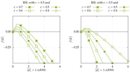
Figure 5.
Preference of different RSL types for green over grey electricity.
Mattes (2012) [32] indicates a WTP for green electricity of RSL ranging from 2.48 ct/kWh for electricity from suppliers with both green and conventional electricity tariffs, to 3.59 ct/kWh for electricity from suppliers with exclusively green electricity tariffs. The WTP even increases to 8.44 ct/kWh if the supplier verifiably invests in RES. Schmuecker (2015) [33] indicates a WTP for green electricity of +15% compared to the grey electricity tariff. Based on an average tariff of 28 ct/kWh, this results in a WTP of 4.2 ct/kWh. The Figure 5 proves that the model’s agents reflect these statements in their behaviour.
5.1.2. Decision Stage II: Regional vs. Interregional Purchase
Figure 6 shows selected RSL types and their preference for regional over interregional electricity purchase in an example scenario. The intersection with the abscissa indicates up to which amount of , compared to an interregional grid fee of (what corresponds approximately to the actual transmission grid fee in Germany), regional purchase is preferred. The left side plot shows four exemplary RSL, all with the same cost awareness of , but with a different regional awareness from to . The plot on the right side depicts four exemplary RSL, all with the same regional awareness of , but with a different cost awareness c.
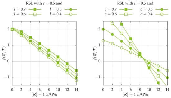
Figure 6.
Preference of different RSL types for regional over interregional purchase.
Surveys or studies on the WTP for regionality, in the sense it is presented in this work, are not available. However, there are several studies that reflect the WTP in a similar context. For example [34] indicate an additional WTP of + 3.50 ct/kwh for electricity supplied by a municipally owned LUC. Mattes (2012) [32] says + 3.41 ct/kwh if the electricity supplier is embedded in the region. Figure 6 shows that the utility functions set up for the model reflect this numbers. At this point, it should be stated that Figure 6 shows the WTP for regional electricity in a comparative presentation to a interregional grid fee of = 8 ct/kWh. That means, according to [32,34] regional purchase is preferred, as long as the regional grid fee does not exceed or 11.50 ct/kWh.
5.2. Individual Review for an RSL Agent
Up to this point, the interdependencies within the REMM are very extensive. This chapter provides a short but precise insight into how the model works in order to get a better understanding on how the overall results accrue. For this purpose, an individual review for one exemplary, selected RSL agent is illustrated in detail.
The observed agent is a pure consumer household characterized by an annual electricity consumption of approximately 2400 kWh, an environmental awareness of e = 0.8, a regional awareness of l = 0.3 and a cost awareness of c = 0.4. Moreover, the threshold value is assumed as . The observation is made for a whole week in month of May (18–24 May 2015). The consumer’s WTP for green over grey electricity results as shown in Section 5.1.1. Taking into account the consumer’s environmental and cost awareness, the consumer is going to purchase green electricity as long as his perception of the price premium for green electricity is less than or equal to 4 ct/kWh. The consumer’s WTP for regional energy purchase results as shown in Section 5.1.2. Assuming an interregional grid fee of and regarding the consumer’s awareness for regionality and costs shown above, the consumer tends to buy a regional product as long as his perception of the regional grid fee is less than or equal to 8.14 ct/kWh.
Figure 7 covers different issues of decision stage I and compares the consumer with a randomly chosen prosumer household operating a PV rooftop system. Thereby, the black graph depicts the hourly electricity demand () of the consumer household. The green graph shows the hourly oversupply () of the prosumer during the same time, whereby the prosumer could act as a potential trading partner for the consumer according to the CA at the regional market selling a green and regional electricity product. Highlighted via dots are specific hours in which the consumers preferences for green over grey electricity were met by the market and the consumer c.p. will purchase green electricity. Red dots indicate beneficial price situations under assumption of perfect price perception (), blue ones under assumption of delayed price perception (). Note, that as the regional grid fee is assumed as a fix price component in this paper’s explanations, it is not necessary to review decision stage II in such detail as it is done for stage I.
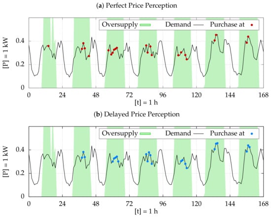
Figure 7.
Beneficial price situations for green electricity purchase of an exemplary RSL agent with (a) perfect perception () and (b) delayed perception ().
Various phenomena can be observed in Figure 7. (I) Within PV generation peaks during noon, prices get low enough to incentivise green electricity purchase. And this not only for single hours but also over periods of up to five hours. (II) Moreover, it can be observed that green energy purchase is even incentivised in hours with relatively low electricity demand. This creates opportunities to shift demand from periods of high electricity consumption to hours of low consumption, what leads into two positive effects. On the one hand, consumers can buy electricity at times and prices that suit their preferences. On the other hand, the local distribution grid is unburdened by shifting peak loads into hours with high generation. (III) These phenomena just mentioned occur irrespective of whether price perception is perfect or delayed.
5.3. Initial Values and Parameters
The aim of this papers overall analysis is to make a first estimation in which direction the results will develop and to uncover potentials for further, more detailed analyses. Therefore, the set up price mechanism is compared with an appropriate reference scenario including fixed electricity tariffs. To investigate the effects of the supply-dependent, flexible price premium for green electricity on the local distribution grid, a conservative generation scenario with less RES is deployed.
Table 6 reflects the initial values and parameters for this paper’s analysis. Deviation from load profile describes the fluctuation range in which each agent’s load profile is allowed to vary randomly. This parameter ensures that several agents of the same type and with the same scaling factor have different consumption values. Furthermore, it generates load peaks and deltas within the load curve. Share of PV and share of CHP indicate how many agents of each type operate a PV respectively a CHP unit, whereas, share of biogas gives the information on the share of CHP units which where driven with biogas. The perception of price components λ is set to 1, the threshold value Δ for switching electricity products is set to 0. The price components of the fix price scenario shown below resemble the actual amount of those components in reality, except of which is an counterfactual component. The amount of is the authors own assumption according to the actual grid fee and an average value for the WTP for regional products. The flex price scenario differs in only one parameter, namely , which results depending on the amount of green electricity generated. Preliminary calculations have shown, that the maximum amount of green energy generated in the REMM, gets up to at most 50% of the actual installed capacity. The LUC calculates the share of electricity generated in relation to installed capacity and sets the price accordingly. The resulting price curve is linear and ranges from 6.5 ct/kWh to 2 ct/kWh.
Table 6.
Initial values and parameters.
Moreover, the distribution of preferences among the agents is decisive for the model’s outcome. To avoid that the outcome is pushed into a direction an approximately uniform distribution was used. Figure 8 displays this distribution exemplary for all 15,407 RSL agents in a histogram over 10 model set-ups. The value of the preference is shown on the abscissa, whereas the ordinate indicates the number of agents characterised by this attribute.
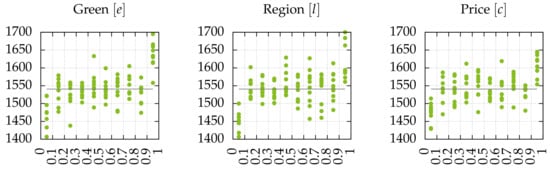
Figure 8.
Uniform distribution of consumer preferences.
The distribution in Figure 8 appears not to be uniform. This results out of the model’s code. The histogram groups the preferences to one decimal place. Because of the model’s formulas (division by zero), a preference cannot have the value 0. So, the first group in the histogram is smaller than the rest and that is why it seems that there are less agents with these preferences. Furthermore, random variables are used to achieve an approximately equal distribution of preferences across all agents in the model. For reasons of model language, it follows that the last group in the histogram contains slightly more agents than the other groups.
5.4. Fix vs. Flex Price Scenario
The following explanations embrace statements and results that apply to the entire supply system, i.e., across all agent groups. The presented results were obtained in a potential assessment study for the REMM, which was carried out to test the model’s basic idea and functions, uncover potentials and develop detailed analysis goals. Results from 5 model runs were processed to depict the general outcome of the model.
First, the reference scenario including fixed electricity tariffs is considered. Figure 9 provides an overview regarding the overall demand for the “green regional” electricity product, the generation of green electricity within the supply system and the leftover sales volume after the consumption of self-generated green electricity, in (a) over one whole year and in (b) over an exemplary week in May.
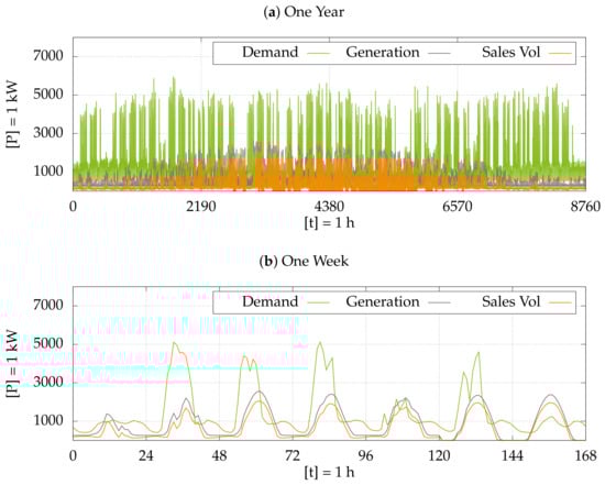
Figure 9.
Green electricity demand, generation and sales volume in fix price scenario over (a) one year (1 January 2015–31 December 2015) and (b) one week (18–24 May 2015).
Though there is green electricity generated by CHP units, the generation graph shows a typical PV-driven profile in (a) with a seasonal peak in summer and in (b) with daily peaks over noon. In contrast, the demand curve seems not to be influenced by the seasonality of generation, rather, it appears that there is a slight decrease in green electricity demand over summer. The daily observation (b) depicts extraordinary demand patterns especially on Monday (hours 0–24) and Friday (hours 96–120). Surprisingly, demand approximately equals sales volume in several hours at noon on these days. Whereas on the other days, the demand curve takes the expected progression but does not equal the sales volume. On Sunday there is less demand than volume, on Tuesday till Thursday and Saturday demand exceeds sales volume. What hits the eye first on these days, is that there is an temporal offset between peak of demand and peak of generation.
Figure 10 shows the comparison between demand for green electricity in fix and flex price scenario, again in (a) over a whole year and (b) over one week. Both graphs display an increase in demand for green electricity. This increase is mainly PV-driven because it occurs seasonally in summer in (a) and daily at noon in (b). Even then the demand exceeds the sales volume partially perceptibly, this increase indicates a great potential for the system integration of RES. Furthermore, it is noticeable in (b) that the temporal offset is reduced by the increase of demand, especially in the afternoon. In general, (b) depicts an enhanced exploitation of regional generation capacities, here again especially in the afternoon. Remarkably is the adjustment of demand on Sunday.
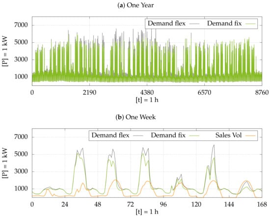
Figure 10.
Green electricity demand in fix and flex price scenario over (a) one year (1 January 2015–31 December 2015) and (b) one week (18–24 May 2015).
Table 7 displays the average market results for the product “Green Regional” in fix and flex price scenario and confirms the conclusions given above. The table is divided into two sections (I) hours with oversupply and (II) hours with undersupply. (I) Hours with regional oversupply of green electricity could be reduced from 712 in fix price scenario to 579 in flex price scenario. Whereas in the fixed electricity tariff scenarios about 318.3 MWh of green, regional electricity were sold to the interregional wholesale energy market by the LUC, in flexible price scenarios only 192.7 MWh were given away. This means a reduction from 7 to 4% of the total green electricity generation. Also the maximum amount of leftover electricity sold in an hour could be reduced from 1.6 MW to 1.1 MW. The average hourly amount could be reduced from 0.44 MW to 0.33 MW.
Table 7.
Market results of product “Green Regional”.
In terms of sustainability, the question arises whether the increased demand for green, regional electricity lowers the demand for grey, regional electricity. Results here are not completely conclusive and vary from run to run, what in average leads to similar results in fix and flex price scenario, as shown in Table 8. By now it seems that there is a direct influence by an increased demand for green electricity on the purchase of grey electricity. Unfortunately, this influence cannot be recognized directly because there is an countering influence induced by the conservative generation scenario and the market clearing mechanism, too. So, the WTP of some agents is met by decreasing prices for green electricity who would normally purchase grey and regional electricity. The problem is the huge amount of agents who also try to purchase the grey and regional product, but are not served because of the relatively low capacity and who are forced to switch to the grey and interregional product. Even if some agents choose to switch from grey to green, there are even more agents who then would not be forced to switch from regional to interregional, so that it appears that there is no change in the purchase of the grey and regional product. Further investigations have to be done.
Table 8.
Market results of product “Grey Regional”.
6. Discussion
The REMM, as an approach of fortifying the regional trading of regionally generated electricity based on cellular structures and flexible energy price components, shows promising results. At first, the investigation of individual agents was started in small steps. By contrasting the single utility functions of the agents, their WTP for green over grey respectively regional over interregional electricity was determined and displayed (see Section 5.1, Figure 5 and Figure 6) comparative for an exemplary RSL agent. It is shown that the utility functions set up, depict the WTPs given in the literature, what enables the REMM to reflect realistic market behaviour. However, it has to be stated that large spreads between the variables e and c respectively l and c can result in an immense WTP, which cannot be assumed for reality this way. Since these high WTPs are not actually called at the market, but prices are capped by the LUC and the individual WTPs only serve for classification in the model, it is legitimate to work with these functions. Note that, if scenarios are considered in which the LUC does not cap prices, the modeller can intervene manually and limit the described spreads in the model code, so that applies: respectively .
Section 5.2 contains an individual review of an exemplary RSL agent, characterised by a high preference for green electricity, a moderate cost sensitivity and a minor preference for regionality. The agent’s market behaviour is examined under perfect and delayed price perception. This investigation serves on the one hand to examine the impact of price perception and on the other hand to prove that preference-based trading takes place within the REMM. Figure 7 indicates that there is a slight influence in the temporal call of the purchase in case of delayed price perception. But, in the overall picture results remain the same irrespective of whether price perception is perfect or delayed.
Moreover, this figure displays, that generation-related electricity prices lower of course at noon when PV generation is at peak and incentivise preference-based electricity trading. This incitement of trading happens independent of the agent’s current demand, and moreover, not only for single hours, but also for periods up to five hours. It is not in the paper’s focus to investigate the effects of load shifting but at this point there is considerable scope for further investigation and intensification in this field of research. It seems that statements in [21], which were made from a technical point of view, can be supported by the REMM from an economic perspective.
These results could not only be obtained for individual agents, but are also confirmed by the investigations for the whole region as shown in Section 5.4. By comparing the model region once in a fix price scenario similar to the reality, and then in a flex price scenario, the differences between the real world and the model’s counterfactual market system were investigated to determine the effects of flexible electricity trading.
The flexible price mechanism ensures that the demand for green electricity increases within the region, both seasonally during the summer and daily at generation peaks. Furthermore, the temporal offset between consumption and generation is reduced, without any technical demand side management, but only via the price. The number of hours with a regional oversupply of green electricity as well as the average and maximum amount of green energy transferred to the superordinate grid level could be reduced. As Figure 10 shows, the demand curve could even be adjusted nearly exactly to the generation in some days.
In this model situation, generation and demand are basically too far apart for a pure market mechanism to match them completely. Even if hours of oversupply can be reduced, this will artificially generate c.p. hours of undersupply. In order to exploit the regional generation capacities to a bigger extend, technical options must be considered in addition to a flexible pricing mechanism. To this end, model extensions must be installed to allow demand side management to the agents and to create shiftable load potentials via battery storages and flexible loads.
Nevertheless, the presented investigations and results are all based on a very conservative generation scenario combined with a demand situation equally distributed across all preferences. Furthermore, a real existing supply system, which includes all consumer groups with their individual characteristics and which has no disproportionate possibility of green electricity generation (e.g., wind farms, free field PV, pump storages etc.) in the system boundaries, was used as the model’s basis. The REMM is an overall assessment for a whole region and not only the attempt of a district solution. In consideration of all these factors, the study proves that there are possibilities for smoothing the exchange balance to the superordinate grid level by market mechanisms, even within non-privileged distribution grid areas like such in the model. The smoothing potential can be expanded further by exploiting the regional generation capacities with technical solutions like demand side management and storage systems.
7. Conclusions
The individual analysis within the REMM proved that its mechanisms depict the actual WTPs of the consumers and that flexible prices make them adjust their buying behaviour not only for single hours, but also over periods and this independent of the agent’s current demand. Moreover it was shown, that slight delays in price perception do not have a big influence on the model’s outcome.
This paper’s overall investigations prove that regional trading can help to smooth the exchange balance of distribution grid areas, both seasonally and daily, by only exploiting the consumers WTP for several electricity products. In detail, not only the temporal offset between consumption and generation could be reduced, but also the number of hours with regional oversupply of green electricity as well as the average and maximum amount of green energy transferred to the superordinate grid level. Note, that all results shown above were achieved without any demand response or demand side management approaches.
We can state that the CA is not only technically feasible [21], but that there are also general economic advantages. Furthermore, the combination of ABM and the CA has proven a relieving basic effect on the supply system and induces a higher customer satisfaction. The combination of these two approaches was therefore worth the effort and the initial results justify further investigations to expand and elaborate the positive outcomes.
Author Contributions
Conceptualization, T.S. and J.M.; methodology, T.S. and J.M.; software, J.M.; validation, J.M.; formal analysis, T.S. and J.M.; investigation, J.M.; resources, T.S. and J.M.; data curation, J.M.; writing—original draft preparation, J.M.; writing—review and editing, T.S.; visualization, J.M.; supervision, T.S.; project administration, T.S.; funding acquisition, T.S. All authors have read and agreed to the published version of the manuscript.
Funding
This research was funded by Saechsische Aufbaubank grant number 100231936. The APC was funded by MDPI.
Informed Consent Statement
Not applicable.
Conflicts of Interest
The authors declare no conflict of interest. The funders had no role in the design of the study; in the collection, analyses, or interpretation of data; in the writing of the manuscript, or in the decision to publish the results.
Abbreviations
The following abbreviations are used in this manuscript:
| ABM | Agent Based Modelling |
| BML | Business with Measured Load Profiles |
| BSL | Business with Standard Load Profiles |
| CA | Cellular Approach |
| CHP | Combined Heat and Power |
| LUC | Local Utility Company |
| RSL | Residential with Standard Load Profiles |
| PV | Photovoltaic |
| REMM | Regional Energy Market Model |
| RES | Renewable Energy Sources |
| WTP | Willingness To Pay |
Appendix A. Scale Factors for Standard Load Profiles
The definition of the RSL scale factor domain refers to the consumption groups according to [35] focusing the groups DB and DC (annual electricity consumption between 1000 and 5000 kWh). The consumption group DA (annual electricity consumption of less than 1000 kWh) is not considered, since a household electricity consumption of this low amount seems not realistic. This assumption is reinforced by [29] (see Figure A1), which also does not consider this group. The consumption groups DD and DE (annual electricity consumption greater than 5000 kWh) are also not taken into account. BDEW 2019 [29] estimates the average electricity consumption, without consideration of heating electricity consumption, of four-person households or bigger at approximately 4940 kWh annually. A domain greater than 5 therefore does not appear sensible.

Figure A1.
Average electricity consumption by household size (Authors own compilation based on [29]).
Figure A1.
Average electricity consumption by household size (Authors own compilation based on [29]).

The domain of scale factors for BSL agents is determined on the basis of the results of a representative survey by [28]. Fraunhofer ISI et al. (2014) [28] divides the evaluated workplaces into 14 groups and further subgroups. However, a detailed evaluation of frequency distributions of the specific electricity consumptions is only carried out for the first four groups, (I) construction business, (II) office and similar, (III) production and (IV) trade. Figure A2 shows a summary of these results. It is clearly shown that despite very different annual electricity consumption of this individual groups, an accumulation in the range of 1000 to 4000 kWh occurs. As of an annual consumption of greater than 12,000 kWh, the frequency is in the low one-digit percentage range. Therefore a domain of 1 to 12 is applied for the REMM.

Figure A2.
Frequency distribution of the specific electricity consumption by business category (Authors own compilation based on [28]).
Figure A2.
Frequency distribution of the specific electricity consumption by business category (Authors own compilation based on [28]).

Appendix B. Dimensioning of Generation Units
Appendix B.1. Dimensioning of PV Systems
In Section 4.3 it is mentioned that PV systems fit to the agent’s consumption patterns. Therefore, the values shown in Table A1 are used to set up these PV systems, while regarding the structure of the stored weather data and the expected full load hours. Taking into account practicality, a constraint is embedded that PV systems may not be smaller than 3 kW. Furthermore, the model is only allowed to raise power capacities by steps of 250 W.
Table A1.
Specifications of implemented standard PV modules.
Table A1.
Specifications of implemented standard PV modules.
| Property | Value |
|---|---|
| Module Power | 250 W |
| Module Surface | 1.6 |
| Efficiency | 16% |
| Full Load Hours | 1000 h |
| Correction Factor | 1.12 |
| (Inclination , South) |
The following transcription illustrates this dimensioning process which is based on the given values of the PV standard modules in Table A1 and the scaling factor (see Section 4.2, Table 1 and Table 2) for each agents consumption. These factor gives information about the total annual electricity consumption of an agent. A scaling factor of 3.3, for example, represents an total electricity consumption of 3300 kWh/a. According to the predefined expectable full load hours (see Table A1), the capacity of the PV system can be calculated as follows.
Due to the constraints mentioned in Section 4.3 the capacity is at least 3 kW or gets rounded up to the next quarter if larger. With this value and according to the other predefined values (see Table A1) the actual size of the PV system can be calculated.
First, the capacity of each module can be used to calculate the number n of modules needed.
Second, combined with the surface of the modules the overall size of the system can be calculated.
Appendix B.2. Determine Generation of PV
The weather data on solar radiation fed to the REMM (see Section 4.1) consists of two components, direct and diffuse solar radiation, both for horizontal surfaces. The German Weather Service provides these values in the unit W/m. Both are stored summed up in the model’s weather data base (see Table A2) and flow from there into the REMM.
Table A2.
Excerpt Weather Data Base.
Table A2.
Excerpt Weather Data Base.
| Date | Time | Direct Radiation | Diffuse Radiation | Stored in Data Base |
|---|---|---|---|---|
| Monday, 20 July 2015 | 04:00–05:00 | 0 W/m | 0 W/m | 0 W/m |
| Monday, 20 July 2015 | 05:00–06:00 | 6 W/m | 13 W/m | 19 W/m |
| Monday, 20 July 2015 | 06:00–07:00 | 19 W/m | 68 W/m | |
| ⋮ | ⋮ | ⋮ | ⋮ | ⋮ |
| Monday, 20 July 2015 | 15:00–16:00 | 136 W/m | 270 W/m | 406 W/m |
The hourly electricity generation of the PV system is then calculated as the factor of the summed up solar radiation, the overall size of the system, the efficiency () and, since the data is for horizontal surfaces, the correction factor for inclination (). Exemplary for the data shown in the last row of Table A2 the generation results as follows.
Appendix B.3. Dimensioning of CHP Units
The dimensioning of the CHP units is less complex than for PV systems and depends only on the annual electricity consumption of the operating agent and the expectable full load hours of these units. Moreover, the rounding rules have to be regarded which were set to respectively . Note that even though these units are operated in a heat-controlled mode, electrical power plays the decisive role in the dimensioning process of the REMM. To give a short example:
Appendix C. Data
Appendix C.1. URLs for Information and Data Download
- NetLogo
- Weather Data
- Standard Load Profiles
Appendix C.2. Coordinates and Number of Agents per Patch
Figure A3 shows the model’s patched supply system and provides information about the geographical coordinates (WGS 84) and the number of RSL, BSL and BML agents.

Figure A3.
Details of the model’s supply system.
Figure A3.
Details of the model’s supply system.

References
- Mueller, T. The Role of Demand Side Management for the System Integration of Renewable Energies. In Proceedings of the 14th International Conference on the European Energy Market (EEM), Dresden, Germany, 6–9 June 2017. [Google Scholar]
- Ringler, P.; Schermeyer, H.; Ruppert, M.; Hayn, M.; Bertsch, V.; Keles, D.; Fichtner, W. Decentralized Energy Systems, Market Integration, Optimization. In Produktion und Energie; KIT Scientific Publishing: Karlsruhe, Germany, 2016. [Google Scholar]
- Rosenkranz, G. Energiewende und Dezentralitaet: Die Treiber. In Energiewende und Dezentralitaet. Zu den Grundlagen einer Politisierten Debatte; Agora Energiewende: Berlin, Germany, 2017; pp. 15–23. [Google Scholar]
- Klobasa, M.; Erge, T.; Bukvic-Schaefer, A.; Hollmann, M. Demand Side Management in dezentral gefuehrten Verteilnetzen (Erfahrungen und Perspektiven). In Proceedings of the 11th Kasseler Symposium on Energy Systems Technology, Information and Communication Technologies for tomorrow’s Energy Supply, Kassel, Germany, 9–10 November 2006; pp. 115–134. [Google Scholar]
- Ladwig, T. Demand Side Management in Deutschland zur Systemintegration erneuerbarer Energien. Ph.D. Thesis, Technische Universitaet Dresden, Dresden, Germany, 2018. [Google Scholar]
- Hillemacher, L.; Hufendiek, K.; Bertsch, K.; Wiechmann, H.; Gratenau, J.; Jochem, P.; Fichtner, W. Ein Rollenmodell zur Einbindung der Endkunden in eine smarte Energiewelt. Z. Energiewirtsch. 2013, 37, 195–210. [Google Scholar] [CrossRef][Green Version]
- Kahla, F.; Holstenkamp, L.; Mueller, J.; Degenhart, H. Entwicklung und Stand von Buergerenergiegesellschaften und Energiegenossenschaften in Deutschland. In Arbeitspapierreihe Wirtschaft & Recht Nr. 27; Leuphana Universitaet Lueneburg: Osnabrueck, Germany, 2017. [Google Scholar]
- Flaute, M.; Großmann, A.; Lutz, C. Gesamtwirtschaftliche Effekte von Prosumer-Haushalten in Deutschland; Discussion Paper; Gesellschaft fuer Wirtschaftliche Strukturforschung mbH (GWS): Osnabrueck, Germany, 2016. [Google Scholar]
- Erdmann, G.; Graebig, M.; Pyka, A.; Yadack, M. SW-Agent-Die Rolle von Stadtwerken in der Energiewende. In Eine agentenbasierte Simulation der Interaktion und Akzeptanz der kommunalen Akteure; Technische Universitaet Berlin and Universitaet Hohenheim: Berlin/Hohenheim, Germany, 2016. [Google Scholar]
- Graichen, P.; Zuber, F. Regionale Gruenstromvermarktung. In Energiewende und Dezentralitaet. Zu den Grundlagen Einer Politisierten Debatte; Agora Energiewende: Berlin, Germany, 2017; pp. 81–92. [Google Scholar]
- Ropenus, S. Regionale Verteilung von Erzeugung und Verbrauch. In Energiewende und Dezentralitaet. Zu den Grundlagen einer Politisierten Debatte; Agora Energiewende: Berlin, Germany, 2017; pp. 57–81. [Google Scholar]
- Ropenus, S. Smart Grid und Smart Market. In Energiewende und Dezentralitaet. Zu den Grundlagen Einer Politisierten Debatte; Agora Energiewende: Berlin, Germany, 2017; pp. 93–114. [Google Scholar]
- Fekete, P. Redispatch in Deutschland-Auswertung der Transparenzdaten April 2013 bis einschließlich September 2020. BDEW 2020. Available online: https://www.bdew.de/media/documents/2020_Q3_Bericht_Redispatch.pdf (accessed on 27 November 2020).
- Lueth, A.; Weibezahn, J.; Zepter, J. On Distributional Effects in Local Electricity Markets Designs-Evidence from a German Case Study. Energies 2020, 13, 1993. [Google Scholar] [CrossRef]
- Nicolson, M.; Fell, M.; Huebner, G. Consumer demand for time of use electricity tariffs: A systematized review of the empirical evidence. Renew. Sustain. Energy Rev. 2018, 97, 276–289. [Google Scholar] [CrossRef]
- Jordehi, A. Optimisation of demand response in electric power systems, a review. Renew. Sustain. Energy Rev. 2019, 103, 308–319. [Google Scholar] [CrossRef]
- Zhou, Z.; Zhao, F.; Wang, J. Agent-Based Electricity Market Simulation with Demand Response from Commercial Buildings. IEEE Trans. Smart Grid 2011, 4, 580–588. [Google Scholar] [CrossRef]
- Mainzer, K. Analyse und Optimierung urbaner Energiesysteme. Ph.D. Thesis, Karlsruher Institut für Technologie (KIT), Karlsruhe, Germany, 2018. [Google Scholar]
- Weinand, J. Energy System Analysis of Energy Autonomous Municipalities. Ph.D. Thesis, Karlsruher Institut für Technologie (KIT), Karlsruhe, Germany, 2020. [Google Scholar]
- Pokropp, M. Agentenbasierte Netzwerkgetriebene Simulation Umweltbewusster Konsumentenentscheidungen: Eine Modellgestuetzte Analyse Sozialer Einfluesse mit einer Anwendung auf den Oekostrombezug von Privathaushalten. Ph.D. Thesis, Technische Universitaet Dresden, Dresden, Germany, 2012. [Google Scholar]
- Verband der Elektrotechnik, Elektronik und Informationstechnik e. V. (VDE). Der Zellulare Ansatz—Grundlage einer Erfolgreichen, Regionenuebergreifenden Energiewende; VDE: Frankfurt am Main, Germany, 2015. [Google Scholar]
- Kiessling, A. Available online: http://www.energycells.eu/zellularer-ansatz (accessed on 13 December 2017).
- Moest, D.; Fichtner, W. Einfuehrung zur Energiesystemanalyse. In Energiesystemanalyse; Universitaetsverlag Karlsruhe: Karlsruhe, Germany, 2009; pp. 11–31. [Google Scholar]
- Genoese, M. Energiewirtschaftliche Analysen des Deutschen Strommarkts mit Agentenbasierter Simulation, 1st ed.; Nomos: Baden-Baden, Germany, 2010. [Google Scholar]
- Hamill, L.; Gilbert, N. Agent-Based Modelling in Economics, 1st ed.; Wiley: Chichester, West Sussex, UK, 2016. [Google Scholar]
- Demazeau, Y. From interactions to collective behaviour in agent-based systems. In Proceedings of the 1st European Conference on Cognitive Science, Saint-Malo, France, April 1995; pp. 117–132. [Google Scholar]
- Kruse, S. Komponentenbasierte Modellierung und Simulation lernfaehiger Agenten. Ph.D. Thesis, Universitaet Hamburg, Hamburg, Germany, 2014. [Google Scholar]
- Fraunhofer ISI; IfE TUM; GfK GmbH; IREES GmbH. Energieverbrauch des Sektors Gewerbe, Handel, Dienstleistungen (GHD) in Deutschland fuer die Jahre 2011 bis 2013; Zwischenbericht an das Bundesministerium fuer Wirtschaft und Technologie (BMWi); ISI: Karlsruhe/München/Nürnberg, Germany, 2015. [Google Scholar]
- BDEW-Bundesverband der Energie und Wasserwirtschaft e.V.: Energiemarkt Deutschland 2019. 2019. Available online: https://www.bdew.de/media/documents/Pub_20190603_BDEW-Energiemarkt-Deutschland-2019.pdf (accessed on 14 November 2019).
- Destatis-Statistisches Bundesamt. Bevoelkerung und Erwerbstaetigkeit: Haushalte und Familien. In Ergebnisse des Mikrozensus 2018; Destatis-Statistisches Bundesamt: Wiesbaden, Germany, 2019. [Google Scholar]
- Statistisches Landesamt des Freistaates Sachsen. Gemeindeblatt: Haushalte, Familien und deren Wohnsituation. In Zensus 2011: Gebietsstand 01.01.2014; Statistisches Landesamt des Freistaates Sachsen: Kamenz, Germany, 2011. [Google Scholar]
- Mattes, A. Gruener Strom: Verbraucher sind bereit fuer Investitionen in erneuerbare Energien zu zahlen. DIW Wochenbericht 2012, 7, 3–9. [Google Scholar]
- Schmuecker, G. Verbraucher wuerden mehr fuer Oekostrom zahlen. Hochschule für Wirtschaft und Umwelt Nürtingen-Geislingen. 2015. Available online: https://idw-online.de/de/news643669 (accessed on 11 November 2019).
- Rommel, J.; Sagebiel, J.; Mueller, J. Quality uncertainty and the market for renewable energy: Evidence from German consumers. Renew. Energy 2016, 94, 106–113. [Google Scholar] [CrossRef]
- Eurostat: Energy Statistics-Electricity Prices for Domestic and Industrial Consumers, Price Components. 2019. Available online: https://ec.europa.eu/eurostat/cache/metadata/en/nrg_pc_204_esms.htm (accessed on 14 November 2019).


Publisher’s Note: MDPI stays neutral with regard to jurisdictional claims in published maps and institutional affiliations. |
© 2021 by the authors. Licensee MDPI, Basel, Switzerland. This article is an open access article distributed under the terms and conditions of the Creative Commons Attribution (CC BY) license (http://creativecommons.org/licenses/by/4.0/).