Relative Stability of Electrical into Mechanical Conversion with BLDC Motor-Cascade Control

Abstract

The conversion of the electrical energy into the mechanical is usually realized by a motor, power electronics and cascade control. The relative stability ($\Theta$-stability), i.e., the displacement of its eigenvalues of this system is analyzed for a drive with a BLDC motor. The influence of changing the basic parameters of the motor and power supply system on the drive operation is considered. 4th order closed-loop transfer-function of the cascade control is presented, where boundaries of the transfer-function coefficients are used. The cascade system which uncertainty of the resistance, inductance, flux and gain parameters is analyzed. Theoretical calculations for the cascade control, simulations and laboratory tests are included in the article.

1. Introduction

Typical uncertainty control problems are presented for one feedback loop, but this paper presents uncertainty analysis for two feedback loops in the cascade control system. This article describes the change in the eigenvalue placement when the parameters of the mathematical model are changed (are uncertain).

Mathematical model parameters in every plant are varying when it works, so they are uncertain. Additionally, the parameters identification method are not perfect, so model parameters are uncertain also. This, uncertainty analysis is very important in every automatic control system. Uncertainty in theory leads to the following methods:

• Classical Nyquist criterion which leads to gain and phase margin [1,2],
• Hardy space ($H_{\infty }$) analysis and synthesis [2,3],
• Kharitonov theorem [4,5],
• relative stability [6,7,8]

In this paper Kharitonov and relative stability are used to cascade control of Brushless Direct Current (BLDC) motor. The motor model is similar to synchronus (with and without permanent magnets), separately-excited DC and induction motor [9]. The closed-loop system eigenvalues for nominal transfer-function parameters of a plant are in certain sector in Gauss’s plane, but if parameters of a plant are uncertain, then sector will be larger—it is relative stability.

The paper presents model of the motor and the cascade system with uncertainty of the resistance, inductance, flux and gain parameters. Moreover, relative stability is analized, thus Kharitonov and $\Theta$-stability theory is used.

Article presents:

• relative stability theory which is more stringent than asymptotic stability [4,6,7,8,10],
• model of BLDC motor with power converter,
• uncertainty of model parameters,
• cascade control system, where transfer-function of the closed-loop system is analyzed, this 4th order function is the basis of $\Theta$-stability analysis in the paper,
• the boundaries of the transfer-function coefficients,
• relative stability analysis of the uncertainty closed-loop cascade control,
• some experimental results of the BLDC motor speed control.

The asymptotic stability testing, but not relative stability, for electric drives is used among other papers [11,12,13,14,15,16].

2. Idea of Relative Stability and Generalization of Routh Theorem

The theory and method for testing relative stability ($\theta$-stability) is described in this section. $\theta$-stability [6] of linear feedback system is described by angle $\theta$ between imaginary axis Im and sector’s band (Figure 1a). Sector $S_{\theta }$ determination for control system poles leads to minimal value of relative damping factor $\xi$, therefore overshoot of step response.

A development method for study stability from [10] is article [6], where has been presented another approach. The linear time-invariant dynamic control system is relatively $\theta$-stability, if all roots of characteristic equation are located inside specified area ($\theta$ angle or damping coefficient $\xi$). In literature [4], this area called $S_{\theta }$.

For characteristic polynomial $M\left(s\right)$, which can be written in a short form:

$$M\left(s\right)=\sum _{k=0}^n{a}_k{s}^k=0$$

(1)

where coefficients $a_k$ have real value, and coefficient $a_n>0$.

If a control system is relatively stable then relative-damping coefficient $\xi$ is greater than the smallest, real relative-damping coefficient results from polynomial coefficient (1):

$$\begin{array}{c}\hfill s={\omega }_0{e}^{j\mathrm{\Psi }}=-\xi {\omega }_0+j{\omega }_0\sqrt{1-{\xi }^2}\\ \hfill \xi =-cos\left(\mathrm{\Psi }\right)=const\end{array}$$

(2)

where: $0\le \xi \le 1$ and ${\omega }_0$ is natural undamping frequency.

For value $\xi$=0 control system described by (1) is stable, because $S_{\theta }$ area, contained all left-half complex variable s (Figure 1). Make substitution as follows:

$$s=\omega e^{j\theta }=\omega e^{j\left(\mathrm{\Psi }-\frac{\pi }{2}\right)}$$

(3)

to (1) received complex polynomial of the variable $\omega$ in the form:

$$M_1\left(\omega \right)=\sum _{k=0}^n{a}_k{e}^{jk\theta }{\omega }^k$$

(4)

The roots of (1) are located from left side of straight line $l_1$ in s-plane (Figure 1a), if all roots of complex polynomial (4) are inside the left-half $\omega$ variable (Figure 1b).

On the other hand, applying substitution:

$$s=\omega e^{-j\theta }=\omega e^{-j\left(\mathrm{\Psi }-\frac{\pi }{2}\right)}$$

(5)

to (1) we can receive the complex polynomial:

$$M_2\left(\omega \right)=\sum _{k=0}^n{a}_k{e}^{-jk\theta }{\omega }^k$$

(6)

The roots of real polynomial (1) are located on the left side of straight line $l_2$ in s-plane, if all roots of after substitution (6) are inside the left-half $\omega$ variable (Figure 1b).

A complex polynomial (4) and (6) are obtained:

$$M_1\left(\omega \right)=\sum _{k=0}^n{a}_k{e}^{jk\theta }{\omega }^k=\sum _{k=0}^n\left(b_k+j{c}_k\right){\omega }^k$$

(7)

$$M_2\left(\omega \right)=\sum _{k=0}^n{a}_k{e}^{-jk\theta }{\omega }^k=\sum _{k=0}^n\left(b_k-j{c}_k\right){\omega }^k$$

(8)

where: $b_k$ and $c_k$ are coefficients in the following form:

$$\begin{array}{c}\hfill b_k=a_{k}cos\left(k\Theta \right)\\ \hfill c_k=a_{k}sin\left(k\Theta \right)\end{array}$$

(9)

where: $k=0,1,2,\cdots ,n$

Polynomial (1), whose roots lie in $S_{\theta }$ area, is relatively $\theta$-stable if and only if $M_1\left(\omega \right)$ or $M_2\left(\omega \right)$ areHurwitz polynomial.

To check, do a polynomials $M_1\left(\omega \right)$ or $M_2\left(\omega \right)$, which have complex coefficients, have all roots with negative real parts, can apply generalization of the Hurwitz criterion, which was discussed in [10], so the Routh criterion generalization can be used, too. The roots of both polynomials (4) and (6) have complex roots, which do not conjugate complex pairs. While roots of $M_1\left(\omega \right)$ are conjugate with correspodning roots of with $M_2\left(\omega \right)$.

In order to study only $\theta$-stability generalization of the Routh criterion, it is necessary to build a modified Routh array, which has real coefficient.

Given polynomials (7) and (8) done multiply both polynomials in order to find real coefficients. Thus, the following polynomial is obtained:

$$D\left(\omega \right)=M_1\left(\omega \right)·M_2\left(\omega \right)=\sum _{i=0}^{2n}{d}_i{\omega }^i$$

(10)

where: $d_i$ are real coefficients:

$$\begin{array}{cc}& d_0=b_0^2+c_0^2\hfill \\ & d_1=2\left(b_0{b}_1+c_0{c}_1\right)\hfill \\ & d_2=b_1^2+c_1^2+2\left(b_0{b}_2+c_0{c}_2\right)\hfill \\ & d_2=2\left(b_1{b}_2+c_1{c}_2\right)+2\left(b_0{b}_3+c_0{c}_3\right)\hfill \\ & ⋮\hfill \\ & d_{2n-1}=2\left(b_{n-1}{b}_n+c_{n-1}{c}_n\right)\hfill \\ & d_{2n}=b_n^2+c_n^2\hfill \end{array}$$

(11)

Using (9), the following relationships are obtained:

$$b_i^2+c_i^2=a_i^2,b_i{b}_j+c_i{c}_j=a_i{a}_{j}cos\left[\left(j-i\right)\theta \right]$$

(12)

After substituting (12) to (11) the coefficients $d_i$ of polynomial $D\left(\omega \right)$ are in the form:

$$\begin{array}{cc}& d_0=a_0^2\hfill \\ & d_1=2a_0{a}_{1}cos\theta \hfill \\ & d_2=a_1^2+2a_0{a}_{2}cos\left(2\theta \right)\hfill \\ & d_3=2a_1{a}_{2}cos\left(\theta \right)+2a_0{a}_{3}cos\left(3\theta \right)\hfill \\ & ⋮\hfill \\ & d_{2n-1}=2a_{2n-1}{a}_{n}cos\theta \hfill \\ & d_{2n}=a_n^2\hfill \end{array}$$

(13)

Thus, the Routh array has $2n+1$ rows:

$$\begin{array}{cccccccccccc}& {\omega }^{2n}\hfill & \hfill |& d_{2n}\hfill & \hfill & d_{2n-2}\hfill & \hfill & \cdots \hfill & \hfill & d_2\hfill & & d_0\\ & {\omega }^{2n-1}\hfill & \hfill |& 2n{d}_{2n}\hfill & \hfill & (2n-2)d_{2n-2}\hfill & \hfill & \cdots \hfill & \hfill & 2d_2\hfill & \\ \hfill & ·\hfill & \hfill |& ·\hfill & \hfill & ·\hfill & \hfill & ·\hfill \\ & ·\hfill & \hfill |& ·\hfill & \hfill & ·\hfill & \hfill & ·\hfill \\ & ·\hfill & \hfill |& ·\hfill & \hfill & ·\hfill & \hfill & ·\hfill & \hfill \\ & {\omega }^0\hfill & \hfill |& d_0\hfill \end{array}$$

(14)

Condition of the $\theta$-stability, using the generalization Routh criterion, is no change of sequence sign:

$$d_{2n},2n{d}_{2n},\dots ,d_0$$

(15)

in the first column of the Routh array (14).

3. Mathemathical Model of BLDC Motor

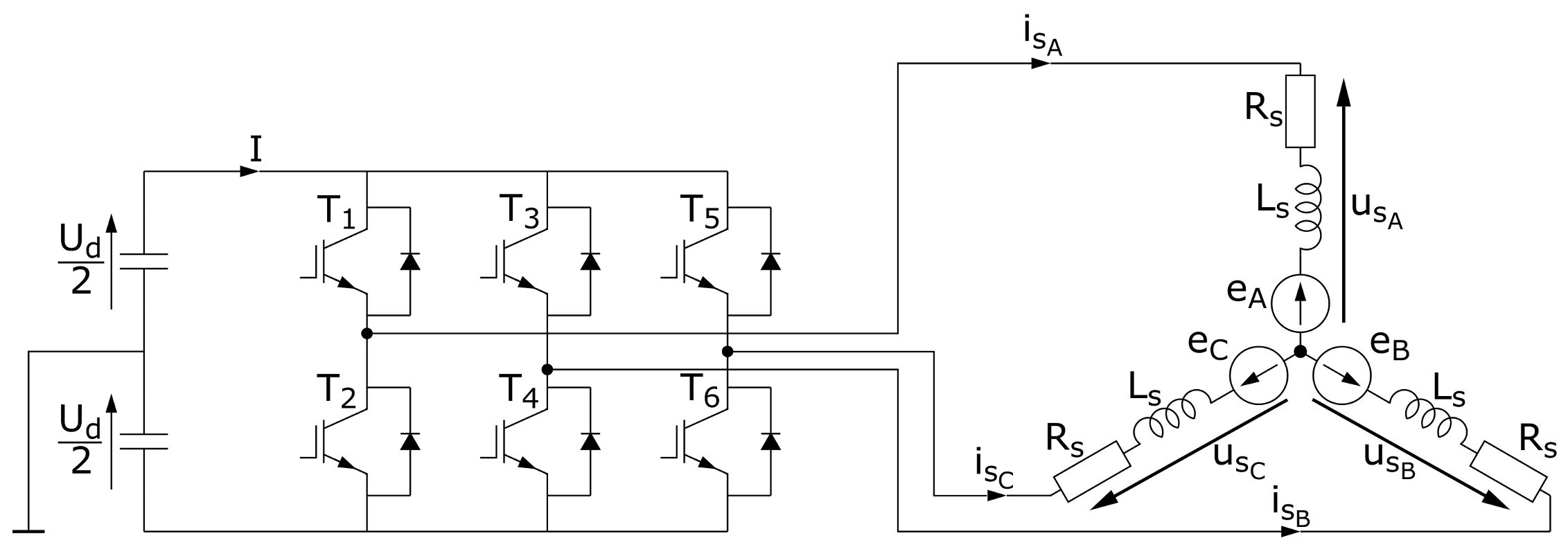
The Figure 2 shows diagram of a BLDC motor supplies by a voltage source inverter.

The mathematical model of BLDC motor is in the following form [17]:

$$\left[\begin{array}{c}{u}_{s_A}\\ u_{s_B}\\ u_{s_C}\end{array}\right]=\left[\begin{array}{ccc}{L}_s-L_{\mu }& 0& 0\\ 0& L_s-L_{\mu }& 0\\ 0& 0& L_s-L_{\mu }\end{array}\right]\left[\begin{array}{c}d{i}_{s_A}/dt\\ d{i}_{s_B}/dt\\ d{i}_{s_C}/dt\end{array}\right]+\left[\begin{array}{ccc}{R}_s& 0& 0\\ 0& R_s& 0\\ 0& 0& R_s\end{array}\right]\left[\begin{array}{c}{i}_{s_A}\\ i_{s_B}\\ i_{s_C}\end{array}\right]+\left[\begin{array}{c}{e}_A\\ e_B\\ e_C\end{array}\right]$$

(16)

where $L_{\mu }$ is mutual inductance between stator coils.

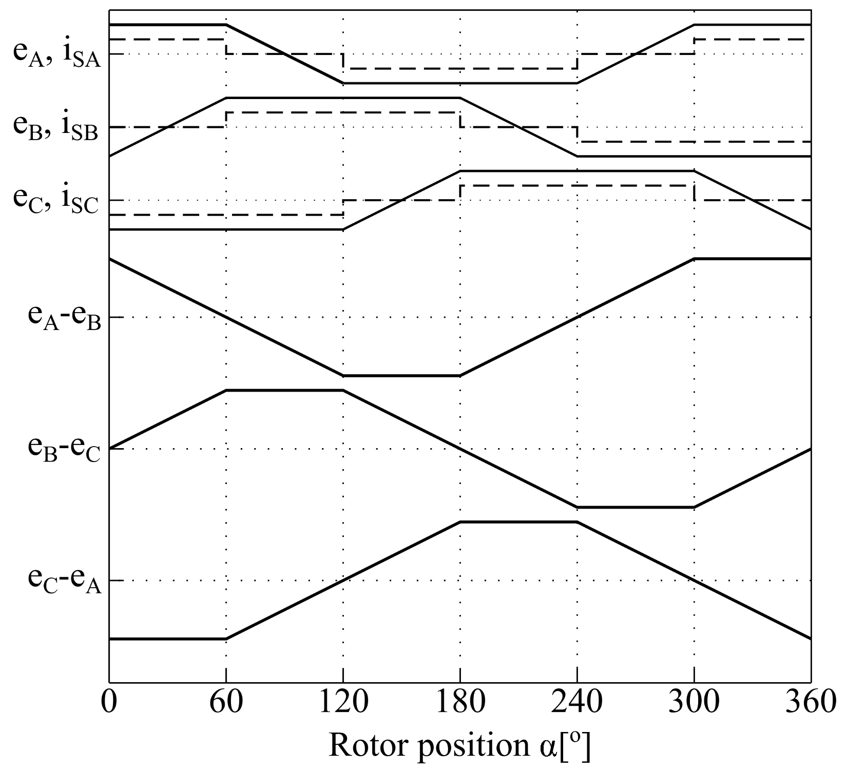
Considering the principle of the motor control (at any moment, the current flows through two stator windings) which result from the design, it is possible to show (present courses of) currents and electromotive forces as in Figure 3, where $\alpha$ is the position of the rotor.

At any time of the control, the current flows through the two stator windings, thus it is assumed:

$$R=2R_S,L=2(L_S-L_{\mu })$$

(17)

The transistors of voltage source inverter (Figure 2) are controlled by the pulse width modulation (PWM) method, with modulation factor $d=0÷1$, so $U\left(t\right)=dUd$.

Finally, the differential equations can be written:

$$\left\{\begin{array}{cc}\hfill & U\left(t\right)=RI\left(t\right)+{\psi }_e\omega \left(t\right)+L\frac{dI\left(t\right)}{dt}\hfill \\ \hfill & J\frac{d\omega \left(t\right)}{dt}=M_e\left(t\right)-M_m\left(t\right)\hfill \\ \hfill & M_e\left(t\right)={\psi }_{e}I\left(t\right)\hfill \\ \hfill & E\left(t\right)={\psi }_e\omega \left(t\right)\hfill \end{array}\right.$$

(18)

where E is back EMF of the two windings, J is moment of inertia, ${\psi }_e$ is permanent magnets flux, $M_e$ is electromagnetic torque, $M_m$ is a load torque.

4. Uncertainty of Model Parameters

The BLDC motor considered in the paper is characterized by a model error, which is due to the uncertainty of the parameters. These errors result from: parameters identification, the conditions and nature of the motor operation.

One of the parameters is the stator windings resistance. This value, apart from the identification errors, changes as the motor temperature increases during operation, according to the relation:

$$R=R_{T_0}[1+\alpha (T_b-T_0)]\mathrm{lub}R=R_{TbN}(1+\alpha \Delta T)$$

(19)

where:

$T_0$ = 293 K⇒ 20 ${}^{\circ }$C,

$T_b$—operating temperature,

$T_{bN}$—rated operating motor temperature, depend on the insulation class,

$\alpha$—temperature coefficient of resistance in Cu $\alpha =4·{10}^{-3}\frac{1}{K}$.

Another parameter that affects the model’s uncertainty is the moment of inertia J, which, in extreme cases can change during operation. For example, a sheet metal reeler. The article omits changes to this parameter.

The inductance of motor windings, which is defined as the ratio of the flux $\psi$ to the current I also contributes to the mathematical model error. In the initial start-up flux and current values change so that their ratio is constant. However, in the further stage of start-up, the flux saturates, while the current arises, which causes the L inductance to decrease.

The above parameters have a particular impact on the values of time constants:

-

$T=\frac{L}{R}$, where T is electromagnetic time-constant,

-

$B=J\frac{R}{{\psi }_e^2}$, where B is electromechanical time-constant,

that directly affect the nature of the drive operation.

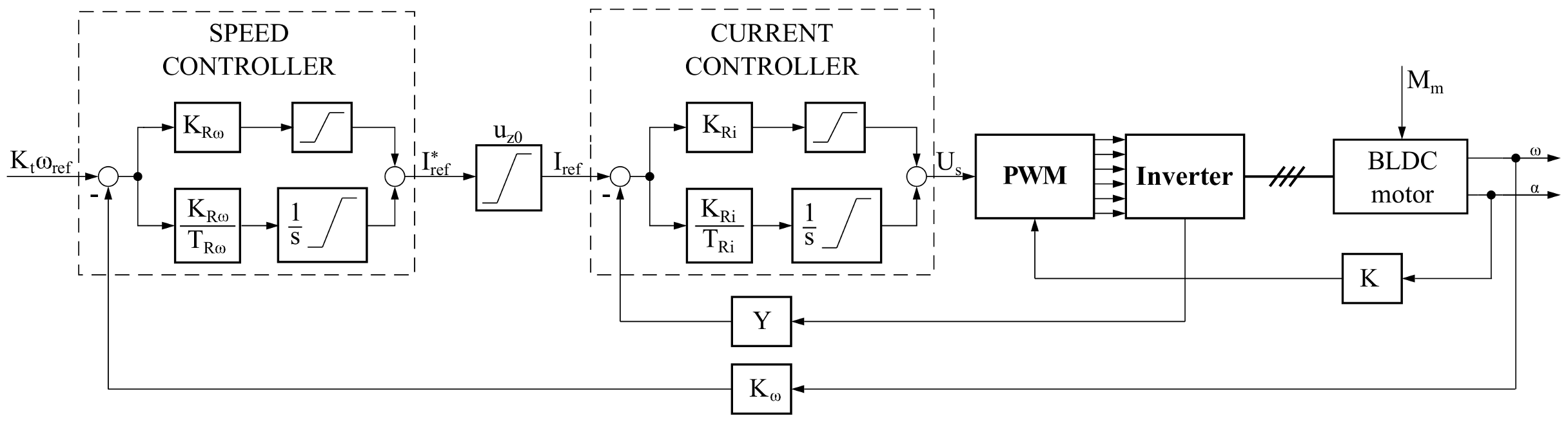
5. BLDC Motor—Speed Control System

Angular speed of the BLDC motor is controlled by using a cascade control structure, where the control of the inverter transistors depends on the current position of the rotor (feedback $K_{\alpha }$). In this type of cascade control, the motor current is usually measured in the intermediate circuit of the inverter, the position of the rotor is measured by the Hall sensors placed on the motor stator, and a incremental encoders are used to measure accurate angular speed.

The control structure shown in Figure 4 consists of a master controller (angular speed control) and the slave controller that is responsible for controlling the electromagnetic torque or quantity proportional to it. In direct current drives, the quantity proportional to the electric torque is the current which is defined as: $M_e={\psi }_{e}I$. The system works in a closed-loop, so that the gains of measuring are also included:

• Y is the gain of the current measuring,
• $K_T$ is the gain of the angular speed measurement ,
• $K_{\alpha }$ is the feedback path, measuring the current position of the rotor.

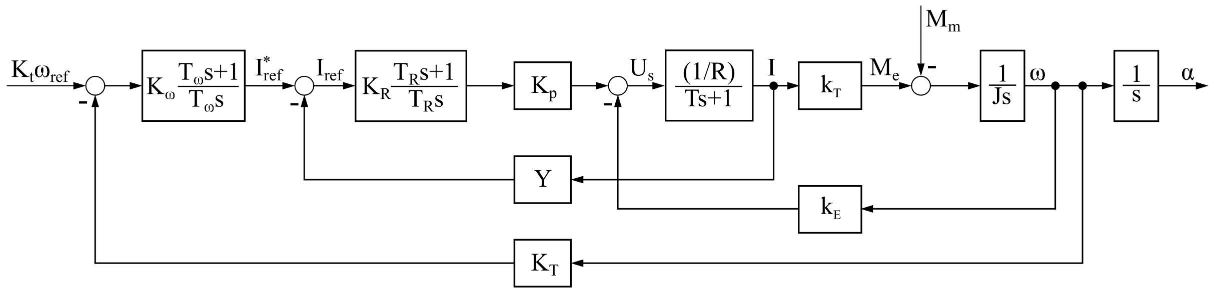
The block diagram of the BLDC drive (Figure 5) was determined from the mathematical model (18), from the diagram in Figure 4 and the inverter gain $K_p$.

The PI current controller assumes the form:

$$G_{RI}\left(s\right)=K_R\frac{T_{R}s+1}{T_{R}s}=\frac{K_R{T}_{R}s+K_R}{T_{R}s}=\frac{ms+1}{Vs}$$

(20)

and the PI speed controller:

$$G_{R\omega }\left(s\right)=K_{\omega }\frac{T_{\omega }s+1}{T_{\omega }s}$$

(21)

Thus, closed-loop transfer-function is equal:

$$G_z\left(s\right)=\frac{\left(K_{\omega }\frac{T_{\omega }s+1}{T_{\omega }s}\right)\left(\frac{\frac{B{K}_{p}m}{R}s+\frac{B{K}_p}{R}}{BTV{s}^2+\left(BV+\frac{B{K}_{p}mY}{R}\right)s+\left(\frac{B{K}_{p}Y}{R}+V\right)}\right)k_T\frac{1}{Js}}{1+K_T\left(K_{\omega }\frac{T_{\omega }s+1}{T_{\omega }s}\right)\left(\frac{\frac{B{K}_{p}m}{R}s+\frac{B{K}_p}{R}}{BTV{s}^2+\left(BV+\frac{B{K}_{p}mY}{R}\right)s+\left(\frac{B{K}_{p}Y}{R}+V\right)}\right)k_T\frac{1}{Js}}$$

(22)

which leads to:

$$G_z\left(s\right)=\frac{b_2{s}^2+b_{1}s+b0}{a_4{s}^4+a_3{s}^3+a_2{s}^2+a_{1}s+a0}$$

(23)

where:

$$\begin{array}{cc}\hfill & b_2=K_{\omega }{T}_{\omega }{k}_T{K}_{p}m\frac{1}{R}\hfill \\ \hfill & b_1=K_{\omega }{T}_{\omega }{k}_T{K}_p\frac{1}{R}+K_{\omega }{k}_T{K}_{p}m\frac{1}{R}\hfill \\ \hfill & b_0=K_{\omega }{k}_T{K}_p\frac{1}{R}\hfill \\ \\ \hfill & a_4=T_{\omega }JTV\hfill \\ \hfill & a_3=T_{\omega }JV+T_{\omega }J{K}_{p}mY\frac{1}{R}\hfill \\ \hfill & a_2=T_{\omega }J{K}_{p}Y\frac{1}{R}+K_{\omega }{T}_{\omega }{k}_T{K}_t{K}_{p}m\frac{1}{R}+T_{\omega }V\frac{k_E^2}{R}\hfill \\ \hfill & a_1=K_{\omega }{T}_{\omega }{k}_T{K}_t{K}_p\frac{1}{R}+K_{\omega }{k}_T{K}_t{K}_{p}m\frac{1}{R}\hfill \\ \hfill & a_0=K_{\omega }{k}_T{K}_t{K}_p\frac{1}{R}\hfill \end{array}$$

(24)

The article considers the uncertainty of the following parameters: $K_p,L,R,{\psi }_e$. By applying the parameter limits (lower or upper) for the denominator coefficients of the closed-system transfer-function, an interval polynomial is obtained in the form:

$$M\left(s\right)=\left[{\underline{a}}_4,{\overline{a}}_4\right]s^4+\left[{\underline{a}}_3,{\overline{a}}_3\right]s^3+\left[{\underline{a}}_2,{\overline{a}}_2\right]s^2+\left[{\underline{a}}_1,{\overline{a}}_1\right]s+\left[{\underline{a}}_0,{\overline{a}}_0\right]$$

(25)

where: ${\underline{a}}_n,{\overline{a}}_n$ are the lower and upper ranges of coefficients (24) and $a_n>0$. Their values are determined according to the following approach:

• boundary coefficient $a_4$ at $s^4$:

  $${\underline{a}}_4=T_{\omega }JV\frac{L_{min}}{R_{max}}$$

  $${\overline{a}}_4=T_{\omega }JV\frac{L_{max}}{R_{min}}$$
• boundary coefficient $a_3$ at $s^3$:

  $${\underline{a}}_3=T_{\omega }JV+T_{\omega }J{K}_{p_{min}}mY\frac{1}{R_{max}}$$

  $${\overline{a}}_3=T_{\omega }JV+T_{\omega }J{K}_{p_{max}}mY\frac{1}{R_{min}}$$
• boundary coefficient $a_2$ at $s^2$:

  $${\underline{a}}_2=T_{\omega }J{K}_{p_{min}}Y\frac{1}{R_{max}}+K_{\omega }{T}_{\omega }{k}_{T_{min}}{K}_t{K}_{p_{min}}m\frac{1}{R_{max}}+T_{\omega }V\frac{k_{E_{min}}^2}{R_{max}}$$

  $${\overline{a}}_2=T_{\omega }J{K}_{p_{max}}Y\frac{1}{R_{min}}+K_{\omega }{T}_{\omega }{k}_{T_{max}}{K}_t{K}_{p_{max}}m\frac{1}{R_{min}}+T_{\omega }V\frac{k_{E_{max}}^2}{R_{min}}$$
• boundary coefficient $a_1$ at s:

  $${\underline{a}}_1=K_{\omega }{T}_{\omega }{k}_{T_{min}}{K}_t{K}_{p_{min}}\frac{1}{R_{max}}+K_{\omega }{k}_{T_{min}}{K}_t{K}_{p_{min}}m\frac{1}{R_{max}}$$

  $${\overline{a}}_1=K_{\omega }{T}_{\omega }{k}_{T_{max}}{K}_t{K}_{p_{max}}\frac{1}{R_{min}}+K_{\omega }{k}_{T_{max}}{K}_t{K}_{p_{max}}m\frac{1}{R_{min}}$$
• boundary coefficient $a_0$:

  $${\underline{a}}_0=K_{\omega }{k}_{T_{min}}{K}_t{K}_{p_{min}}\frac{1}{R_{max}}$$

  $${\overline{a}}_0=K_{\omega }{k}_{T_{max}}{K}_t{K}_{p_{max}}\frac{1}{R_{min}}$$

6. Uncertainly Parameters of BLDC Drive

The BLDC motor drive with the following rated parameters is considered:

• $R_s$ = 5.25 [$\mathrm{\Omega }$]—single-phase resistance,
• $L_s$ = 0.46 [mH]—single-phase inductance,
• E = 2.62 [$\frac{\mathrm{V}}{1000}$$\frac{\mathrm{obr}}{\min }$]—electromotive force,
• $k_T$ = 24.9 [$\frac{\mathrm{mNm}}{\mathrm{A}}$]—torque constant,
• $k_E$ = 24.9 [$\frac{\mathrm{mNm}}{\mathrm{A}}$]—emf constant,
• J = 9.9 ·${10}^{-7}$ [kgm${}^2$]—moment of inertia.

The ranges of the parameters uncertainty for the tests according following forms:

• $R\in [0.5R_N,1.1R_N]\Rightarrow R\in [5.25\mathrm{\Omega },11.55\mathrm{\Omega }]$
• $L\in [0.7L_N,1.1L_N]\Rightarrow L\in [0.644\mathrm{mH},1.012\mathrm{mH}]$
• $Kp\in [0.95K{p}_N,1.3K{p}_N]\Rightarrow Kp\in [1.996\frac{\mathrm{V}}{\mathrm{V}},2.7313\frac{\mathrm{V}}{\mathrm{V}}]$
• ${\mathrm{\Psi }}_e\in [0.85{\mathrm{\Psi }}_{e_N},{\mathrm{\Psi }}_{e_N}]\Rightarrow {\mathrm{\Psi }}_e\in \left[0.0102\frac{\mathrm{Vs}}{\mathrm{rad}},0.012\frac{\mathrm{Vs}}{\mathrm{rad}}\right]$

Thus, the interval polynomial coefficients are:

• $a_4\in \left[2.7174·{10}^{-14},9.3943·{10}^{-14}\right]$
• $a_3\in \left[4.9362·{10}^{-10},5.0621·{10}^{-10}\right]$
• $a_2\in \left[8.1549·{10}^{-8},2.4617·{10}^{-7}\right]$
• $a_1\in \left[7.1677·{10}^{-6},2.5386·{10}^{-5}\right]$
• $a_0\in \left[3.5682·{10}^{-4},1.3·{10}^{-3}\right]$

If the current controller (20) parameters are:

$$\begin{array}{c}\hfill m=0.0879·{10}^{-3},V=0.0123\end{array}$$

(26)

and for velocity controller (21):

$$\begin{array}{c}\hfill K_{\omega }=8.9474,T_{\omega }=0.02\end{array}$$

(27)

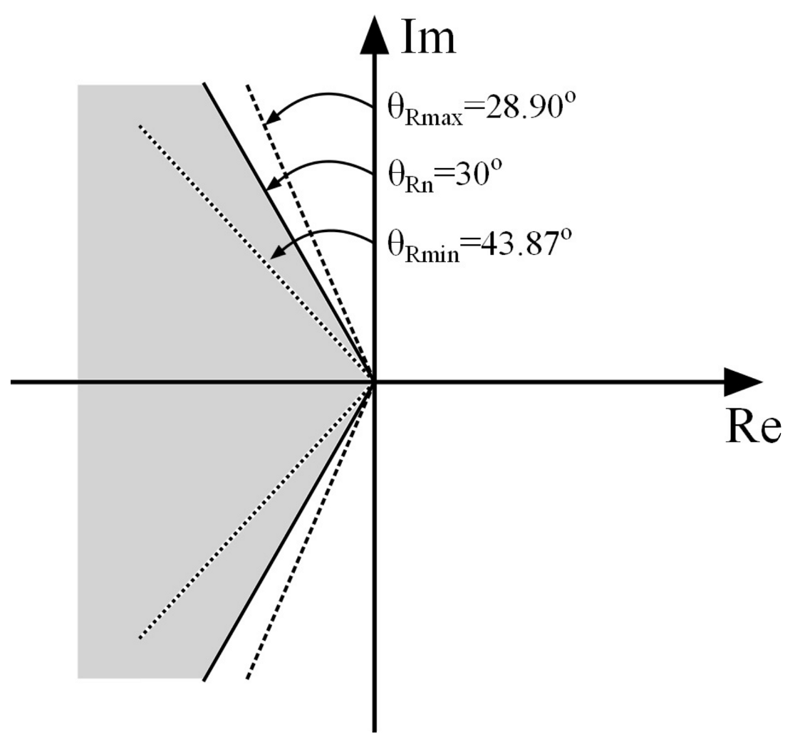
This rated closed-loop transfer-function (23) is:

$$G_N\left(s\right)=\frac{7.87·{10}^{-8}{s}^2+8.998·{10}^{-4}s+0.04479}{4.27·{10}^{-14}{s}^4+4.946·{10}^{-10}{s}^3+9.807·{10}^{-8}{s}^2+9.764·{10}^{-6}s+4.861·{10}^{-4}}$$

(28)

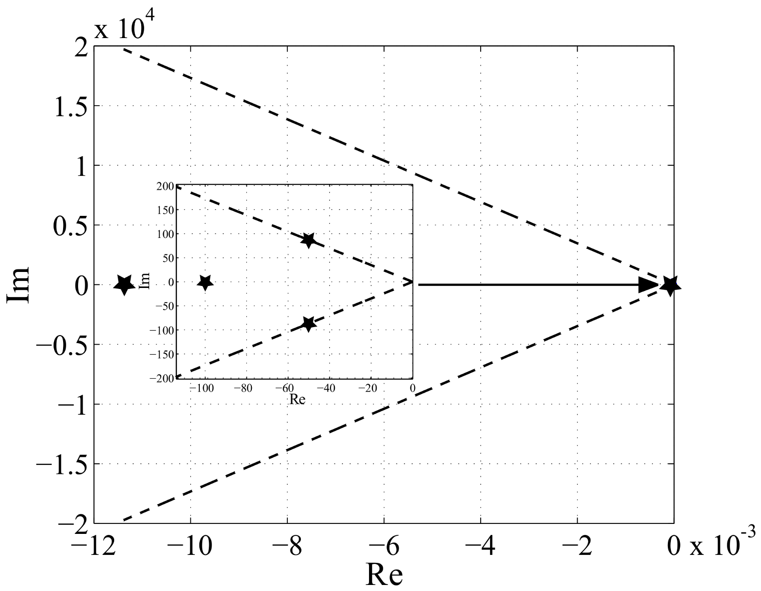
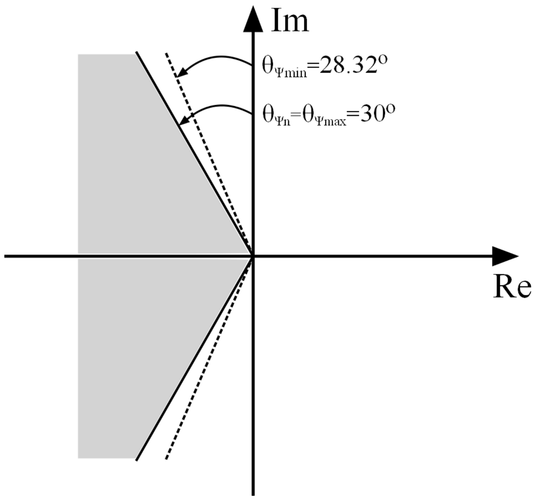
The obtained transfer-function $G_N\left(s\right)$, more precisely the characteristic polynomial, is subjected to algebraic studies of the relative $\theta$ -stability and the value of the relative damping factor is $\xi =0.5$, which corresponds to the angle $\theta ={30}^{\circ }$. Upper values determine the boundary sector of relative stability (Figure 6), “to which the results of changes of individual parameter values will refer”. to which there will be referred the results of the particular parameter value changes.

6.1. Interval of the Stator Resistance

The first uncertain parameter is the resistance of the motor stator, which is in the range:

$$R\in [0.5R_N,1.1R_N]$$

Applying the minimum resistance value $\left(R_{min}\right)$ to the transfer-function coefficients (23) equation can be written:

$$G_{Rmin}\left(s\right)=\frac{1.574·{10}^{-7}{s}^2+1.8·{10}^{-3}s+0.08958}{8.54·{10}^{-14}{s}^4+5.019·{10}^{-10}{s}^3+1.96·{10}^{-7}{s}^2+1.95·{10}^{-5}s+9.72·{10}^{-4}}$$

(29)

Analyzing the denominator of transfer-function (29), we get the relative damping factor $\xi =0.693$, corresponding to the angle $\theta =43.87$${}^{\circ }$. On the other hand, if we use the maximum value of resistance $\left(R_{max}\right)$ to the transfer-function coefficients (23), we obtain the transfer-function of a closed circuit in the form:

$$G_{Rmax}\left(s\right)=\frac{7.155·{10}^{-8}{s}^2+8.18·{10}^{-4}s+0.04072}{3.882·{10}^{-14}{s}^4+4.94·{10}^{-10}{s}^3+8.92·{10}^{-8}{s}^2+8.88·{10}^{-6}s+4.42·{10}^{-4}}$$

(30)

where dumping factor $\xi =0.4524$ and angle $\theta =26.90$${}^{\circ }$.

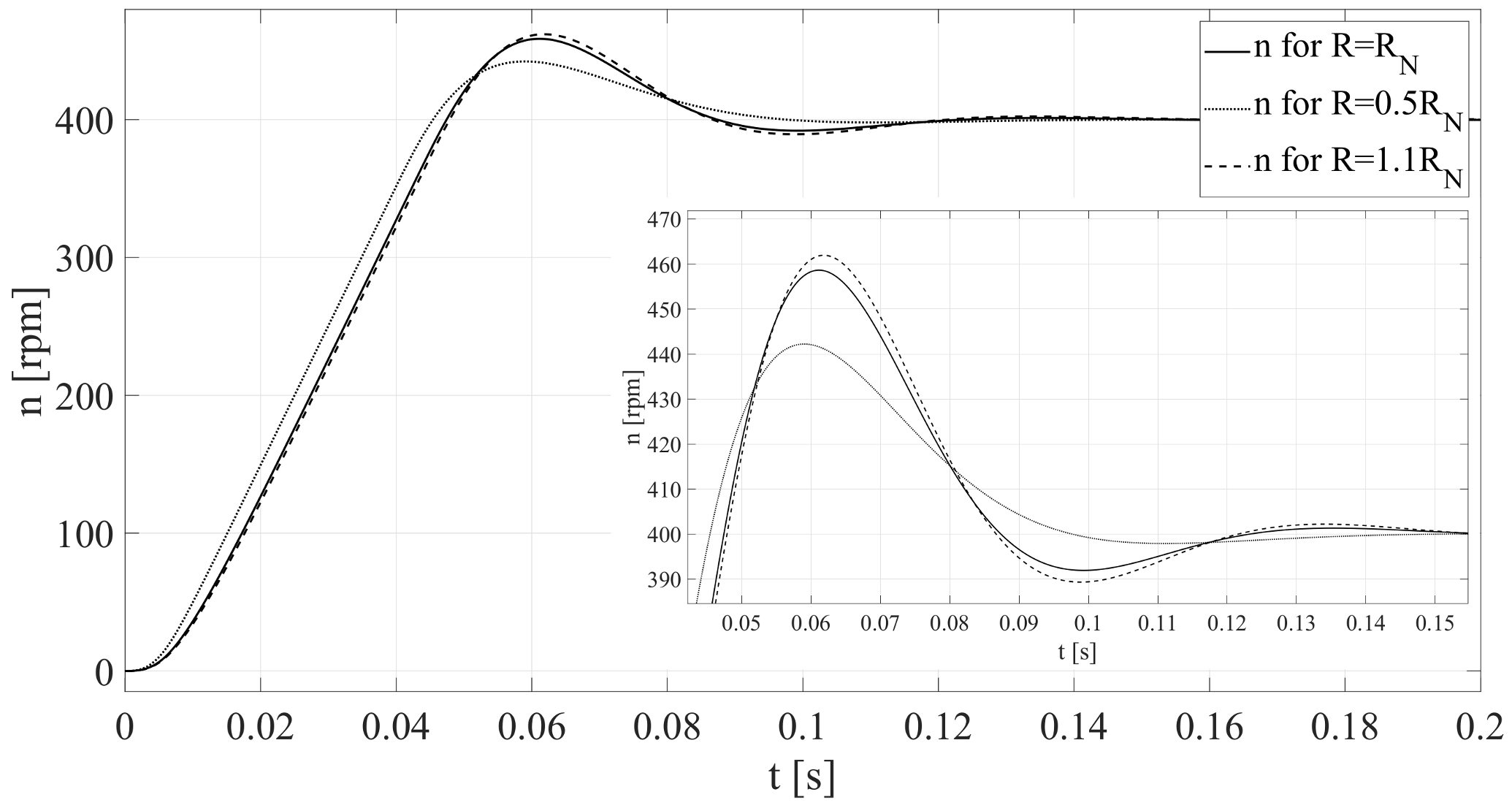
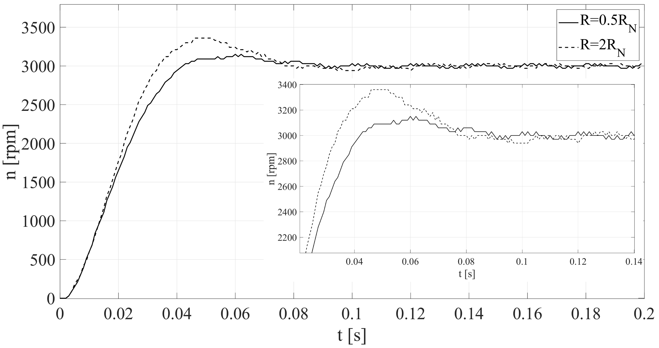
The Figure 7 shows sectors of relative stability determined by characteristic polynomial roots, for different resistance values.

After sector analysis with disturbed parameters and referring them to the nominal sector the system is relative $\theta$-stable for a resistance lower than the nominal one ($R_{min}<R_N$), because this sector is located inside the nominal sector ${\theta }_N$. When the resistance reaches the maximum value of $\left(R_{max}\right)$, study object will lose relative stability because ${\theta }_{R_{max}}$ sector is located outside the nominal sector (all roots aren’t inside the ${\theta }_{R_N}$ sector). Thus, for $R=R_{max}$ the system has greater overshoot and oscillations during start-up than for rated parameters. On the other hand, for the $R=R_{min}$ the system has the smallest overshoot, which is confirmed by the relative damping factor $\xi$.

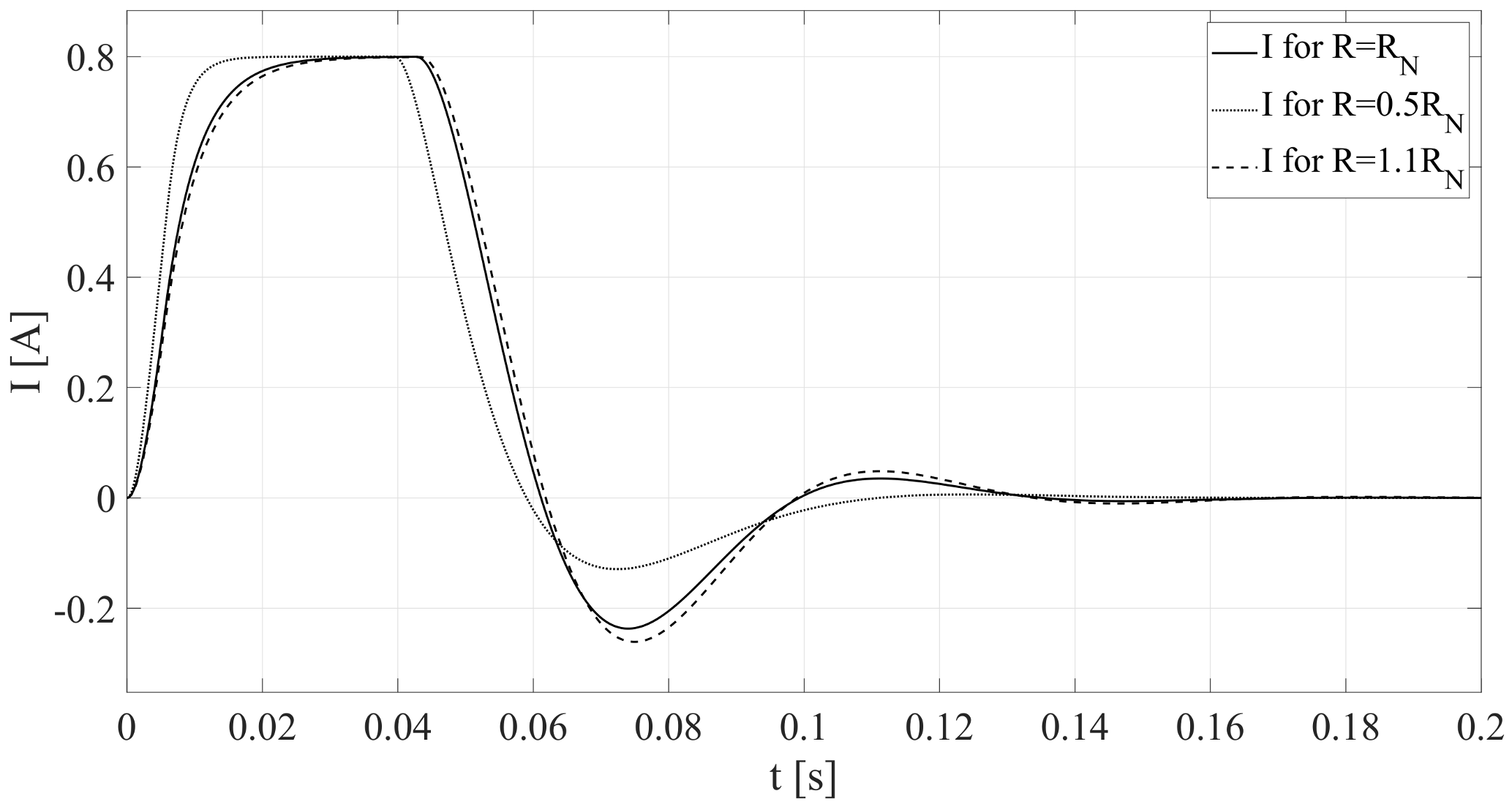
The simulation results (in Matlab environment) obtained for angular velocity (Figure 8) and current of the inverter (Figure 9) confirm $\theta$-stability analysis.

These results confirm validity of the statements regarding relative damping factor $\xi$, whose value represents the overshoot value in the real system. Each waveform, for a resistance value of $R_{min}=5.25\mathrm{\Omega }$, or $\xi =0.693$, has the lowest overshoot, and for a resistance value of $R_{max}=11.55\mathrm{\Omega }$, or $\xi =0.4524$, has the highest overshoot.

Thus, the statements of the relative damping factor $\xi$, whose the value corresponds to the overshoot in the real system, are confirmed (Figure 8 and Figure 9).

6.2. Interval of the Inductance

The range of inductance variation is:

$$L\in [0.7L_N,1.1L_N]$$

thus, transfer-function for $L_{min}$ and $L_{max}$ are in the following forms:

$$G_{Lmin}\left(s\right)=\frac{7.87·{10}^{-8}{s}^2+8.998·{10}^{-4}s+0.04479}{2.989·{10}^{-14}{s}^4+4.95·{10}^{-10}{s}^3+9.81·{10}^{-8}{s}^2+9.764·{10}^{-6}s+4.86·{10}^{-4}}$$

(31)

$$G_{Lmax}\left(s\right)=\frac{7.87·{10}^{-8}{s}^2+8.998·{10}^{-4}s+0.04479}{4.697·{10}^{-14}{s}^4+4.95·{10}^{-10}{s}^3+9.81·{10}^{-8}{s}^2+9.764·{10}^{-6}s+4.86·{10}^{-4}}$$

(32)

After analysing above transfer-functions, we get:

• for (28): $\theta ={30}^{\circ }$,
• for (31): $\theta =29.{95}^{\circ }$,
• for (32): $\theta =30.{013}^{\circ }$.

So $\theta$-stability is always fulfilled and the simulation studies confirmed above results and conclusions.

6.3. Interval of Inverter Gain

The range of variability inverter parameter $K_p$ is determined by the voltage on capacitor in DC circuit:

$$Kp\in [0.95K{p}_N,1.3K{p}_N]$$

where transfer-function (23) for $\left(K{p}_{min}\right)$ assumes form:

$$G_{K{p}_{min}}\left(s\right)=\frac{7.477·{10}^{-8}{s}^2+8.548·{10}^{-4}s+0.04255}{4.27·{10}^{-14}{s}^4+4.94·{10}^{-10}{s}^3+9.39·{10}^{-8}{s}^2+9.276·{10}^{-6}s+4.62·{10}^{-4}}$$

(33)

Analysis of the denominator (33) gives the relative damping factor $\xi =0.4785$ corresponding to the angle $\theta =28.{59}^{\circ }$.

Applying $\left(K{p}_{max}\right)$ substitution, transfer-funtcion (23) is in the following form:

$$G_{K{p}_{max}}\left(s\right)=\frac{1.023·{10}^{-7}{s}^2+1.17·{10}^{-3}s+0.05823}{4.27·{10}^{-14}{s}^4+4.97·{10}^{-10}{s}^3+1.23·{10}^{-7}{s}^2+1.269·{10}^{-5}s+6.32·{10}^{-4}}$$

(34)

where for $\left(K{p}_{max}\right)$ damping factor eqauls $\xi =0.6130$ and angle $\theta =37.{81}^{\circ }$.

Figure 10 shows relative stability sectors determined by the roots of characteristic polynomials for different values of the inverter gain $K_p$.

Analysis of the received sectors with disturbed parameters and reference to the nominal sector, shows that the system is relative $\theta$-unstable for gain value less than nominal ($K{p}_{min}<K{p}_N$), because this sector is located outside of the nominal sector. In second case the gain value is $K{p}_{max}$ and the system is relative stable because the sector ${\theta }_{K{p}_{max}}$ is within the nominal sector. The simulations (Figure 11) confirm the studies results. For $K{p}_{max}$, the control system has the lowest overshoot compared to the speed waveforms at rated and minimum $Kp$ gain value, which is presented in Figure 11.

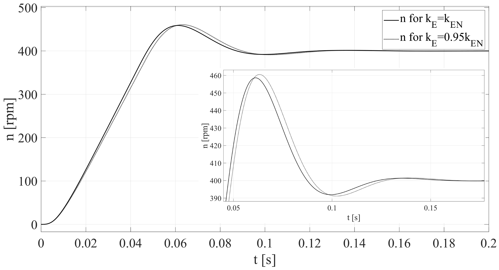
6.4. Interval of the Flux Linkage

The last parameter tested is flux linkage ${\psi }_e$, which takes limit values in the range:

$${\psi }_e\in [0.85{\mathrm{\Psi }}_{e_N},{\mathrm{\Psi }}_{e_N}]$$

and gets a transfer-function for ${\psi }_{min}$:

$$G_{{\psi }_{min}}\left(s\right)=\frac{6.69·{10}^{-8}{s}^2+7.648·{10}^{-4}s+0.03807}{4.27·{10}^{-14}{s}^4+4.95·{10}^{-10}{s}^3+9.387·{10}^{-8}{s}^2+8.3·{10}^{-6}s+4.132·{10}^{-4}}$$

(35)

According to the analysis of the characteristic polynomial (35), the result is $\xi =0.4744$ and $\theta =28.{32}^{\circ }$. This polynomial compared to the characteristic transfer-function polynomial (28) is relative $\theta$-unstable (Figure 12).

The transitions of angular speed, shown in the Figure 13, based on the cascade control structure (Section 5) confirms that the system is $\theta$-unstable for transfer-function (35).

7. Kharitonov Theorem

One of the most popular methods of testing uncertain dynamic systems is the Kharitonov theorem. Unfortunately, successive maximum and minimum values of coefficients in the interval characteristic equations are often mutually exclusive (in one equation). Therefore, the theorem very quickly allows to determine asymptotic or relative stability, but the results are approximate.

The interval polynomial is in the form [18]:

$$P\left(s\right)=[{\underline{a}}_n,{\overline{a}}_n]s^n+[{\underline{a}}_{n-1},{\overline{a}}_{n-1}]s^{n-1}+\cdots +[{\underline{a}}_1,{\overline{a}}_1]s+[{\underline{a}}_0,{\overline{a}}_0]$$

(36)

where $[{\underline{a}}_i,{\overline{a}}_i]$ are a range of uncertain polynomial coefficients and ${\underline{a}}_n>0$.

Theorem 1

(Kharitonov Theorem). Every polynomial $P\left(s\right)$ from the polynomial family (36) is stable if and only if the following four Kharitonov polynomials are stable:

$$\begin{array}{cc}\hfill p_1\left(s\right)& ={\underline{a}}_n{s}^n+{\underline{a}}_{n-1}{s}^{n-1}+{\overline{a}}_{n-2}{s}^{n-2}+{\overline{a}}_{n-3}{s}^{n-3}+{\underline{a}}_{n-4}{s}^{n-4}+{\underline{a}}_{n-5}{s}^{n-5}+\cdots \hfill \end{array}$$

(37)

$$\begin{array}{cc}\hfill p_2\left(s\right)& ={\overline{a}}_n{s}^n+{\overline{a}}_{n-1}{s}^{n-1}+{\underline{a}}_{n-2}{s}^{n-2}+{\underline{a}}_{n-3}{s}^{n-3}+{\overline{a}}_{n-4}{s}^{n-4}+{\overline{a}}_{n-5}{s}^{n-5}+\cdots \hfill \end{array}$$

(38)

$$\begin{array}{cc}\hfill p_3\left(s\right)& ={\underline{a}}_n{s}^n+{\overline{a}}_{n-1}{s}^{n-1}+{\overline{a}}_{n-2}{s}^{n-2}+{\underline{a}}_{n-3}{s}^{n-3}+{\underline{a}}_{n-4}{s}^{n-4}+{\overline{a}}_{n-5}{s}^{n-5}+\cdots \hfill \end{array}$$

(39)

$$\begin{array}{cc}\hfill p_4\left(s\right)& ={\overline{a}}_n{s}^n+{\underline{a}}_{n-1}{s}^{n-1}+{\underline{a}}_{n-2}{s}^{n-2}+{\overline{a}}_{n-3}{s}^{n-3}+{\overline{a}}_{n-4}{s}^{n-4}+{\underline{a}}_{n-5}{s}^{n-5}+\cdots \hfill \end{array}$$

(40)

The stability conditions of the low degrees interval polynomials are given in [5] and for an uncertain fourth-degree polynomial

$$\begin{array}{cc}\hfill P_4\left(s\right)& =[{\underline{a}}_4,{\overline{a}}_4]s^4+[{\underline{a}}_3,{\overline{a}}_3]s^3+[{\underline{a}}_2,{\overline{a}}_2]s^2+[{\underline{a}}_1,{\overline{a}}_1]s^1+[{\underline{a}}_0,{\overline{a}}_0]\hfill \end{array}$$

(41)

The interval polynomial is stable if the following inequalities occur:

$${\underline{a}}_4>0,{\underline{a}}_3>0,{\underline{a}}_2>0,{\underline{a}}_1>0,{\underline{a}}_0>0$$

(42)

and polynomials

$$p_2\left(s\right)={\overline{a}}_4{s}^4+{\overline{a}}_3{s}^3+{\underline{a}}_2{s}^2+{\underline{a}}_1{s}^1+{\overline{a}}_0$$

(43)

$$p_4\left(s\right)={\overline{a}}_4{s}^4+{\underline{a}}_3{s}^3+{\underline{a}}_2{s}^2+{\overline{a}}_1{s}^1+{\overline{a}}_0$$

(44)

are stable, so from Liénarda-Chiparta theorem [18] stability conditions are in the form

$${▵}_{32}={\overline{a}}_3{\underline{a}}_2{\underline{a}}_1-{\overline{a}}_3^2{\overline{a}}_0-{\overline{a}}_4{\underline{a}}_1^2>0$$

(45)

$${▵}_{34}={\underline{a}}_3{\underline{a}}_2{\overline{a}}_1-{\underline{a}}_3^2{\overline{a}}_0-{\overline{a}}_4{\overline{a}}_1^2>0$$

(46)

Thus, stability condition for considered interval polynomial are (42), (45) and (46).

After inserting the coefficients of interval polynomials $a0÷a4$ for Kharitonov’s polynomial (41) there are obtained four polynomials (37), (38), (39) and (40) representing the worst conditions of the BLDC drive:

• for (37): $\theta =0^{\circ }$, $\xi =0$
• for (38): $\theta =1.{83}^{\circ }$, $\xi =0.0319$
• for (39): $\theta =20.{55}^{\circ }$, $\xi =0.3510$
• for (40): $\theta =13.{64}^{\circ }$, $\xi =0.2358$

Comparing received sectors with a nominal sector ${\theta }_{GN}$ (28), the drive is $\theta$-unstable in each case. The results obtained even show the possibility of loss of asymptotic stability by the control system, while the real results are in the open left Gauss’s half plane.

8. Experimental Results

Low power BLDC motor (rated voltage is 15 V, current is 1.1 A) was used in laboratory stand (Motion Control Kit F240 produced by Technosoft in 1998 year [19]), thus the experiments were safe. MCK243 is a complete motion kit, including a voltage source inverter and a three-phase permanent magnet synchronous motor with incremental encoder and Hall sensors. The main element of this kit is the TMS320F243 Digital Signal Processor (DSP) for digital motion control applications.

Unfortunately, not all calculations could be proved practically. The following section presents the change of $K_p$ and R. For a better representation of $\theta$-stability laboratory experiments were realized for an increased range of parameter changes.

Testing the changes of resistance is difficult, so for $2R_N$ additional resistances were used and a start-up was performed. However, for $0.5R_N$, the controllers were optimized for a higher stator resistance, and the experiment was carried out for the rated one—this case is an artificial proof of previous calculations. The experimental results are shown in Figure 14.

Obtained results are similar to presented in Figure 8.

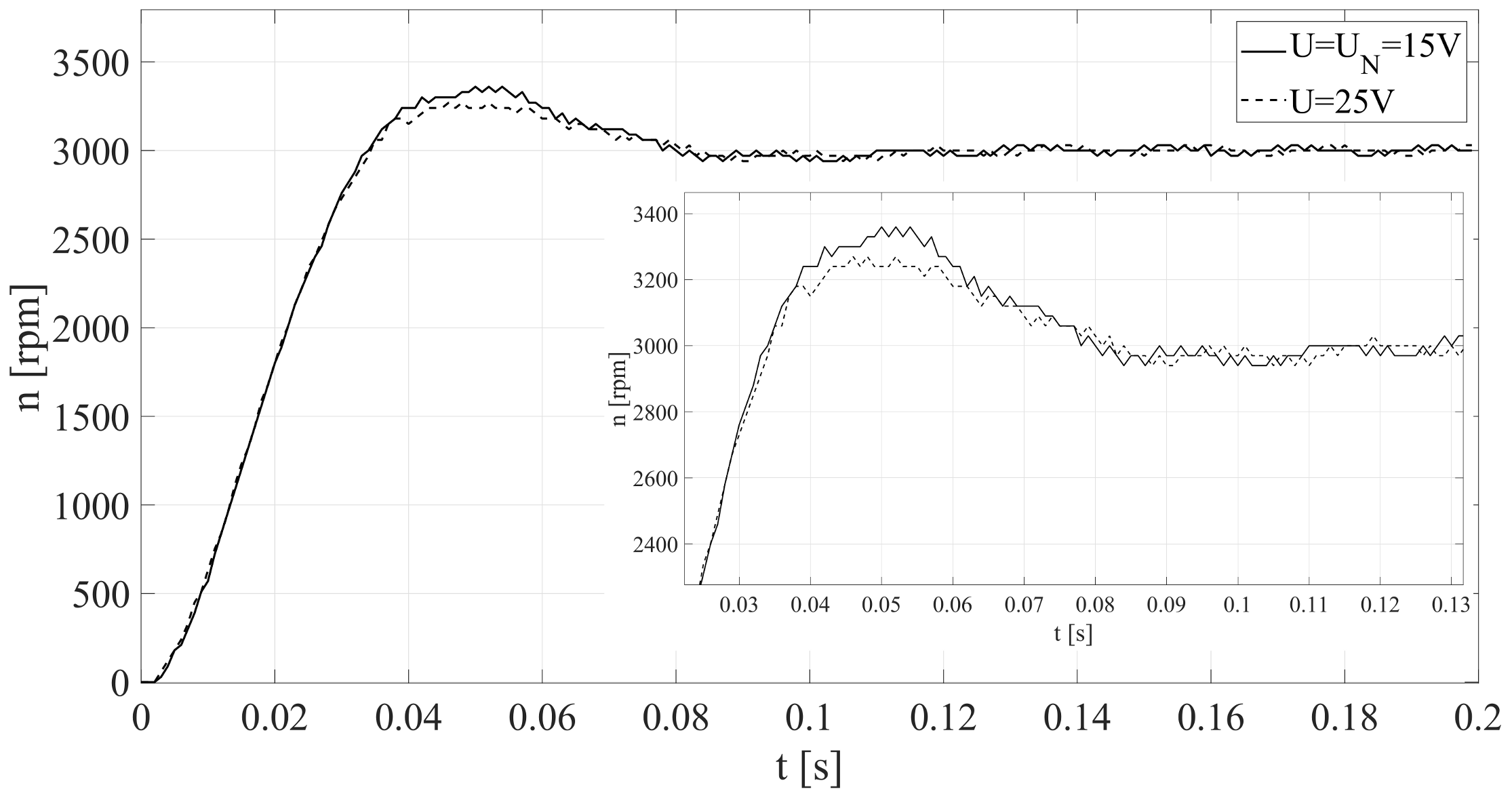
The next stage of laboratory tests was the change of voltage on the capacitor in the DC circuit, which was considered in the analysis as a change $K_p$. Experiments were carried out for 12, 15 and 25 V, again the results for a larger range of parameter changes were observed. The aim was to observe the effects of voltage changes in the DC circuit (Figure 15)—the step responses for 12 V and 15 V are practically the same, so for 12 V is omitted.

Obtained results are similar to presented in Figure 11, so laboratory results confirm previous mathematical analysis.

Experimental verification of the remaining theoretical calculations and simulations is difficult on a real motor, but the presented experiments of uncertainty the most important parameters R, $K_p$ showed the correctness of theoretical calculations.

The next experiments are not as simple because changing the inductance of the motor windings is difficult to implement. For this reason, optimization of the controllers for the incorrectly identified inductance L was done. It was assumed, in the optimization of the controllers where $L=1/0.7{\dot{L}}_N=1.31$ mH (the inverse of the uncertainty assumptions of L) and the experiment was performed for the nominal value of L. The results are shown in Figure 16.

The obtained results slightly differ from the theory, possibly due to the nonlinearity of the low-power motor tested. In addition, the obtained result can be interpreted as: what happens if L is incorrectly identified and used to adjust controllers.

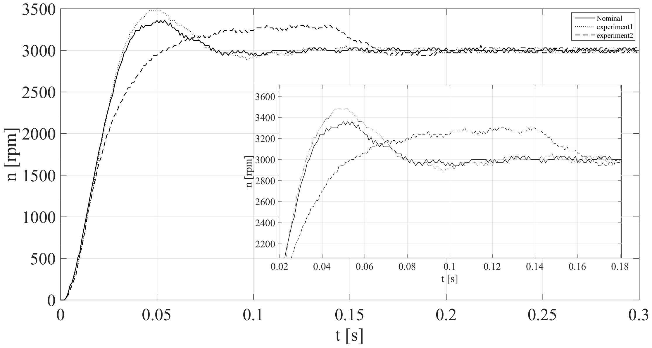
The next step was to introduce multiple perturbations of the motor model parameters to selection of the controllers settings and additionally lower supply voltage was used. Two experiments were realized/prepared for:

(1)

$R=0,5R_N,L=0,5L_N,\psi =0,8{\psi }_N,U=15$ V,

(2)

$R=2R_N,L=1,2L_N,\psi =1,2{\psi }_N,U=10$ V.

The step responses are shown in Figure 17.

Experiment 1 shows less damping ratio than the nominal case, so the system is not $\Theta$-stable. This is similar to the case shown in Figure 18. On the other hand, experiment 2, where the supply voltage is reduced, shows that the obtained signal is deformed (almost flat part for t = 0.06–0.14 s) and this is the effect of voltage limitation which is not considered in the calculation.

9. Conclusions

The analytical approach was used to determine the fourth-order transfer function for a cascade control system with a BLDC motor, for which the limits of changes of the numerator and denominator coefficients were determined.The denominator polynomial was used to calculate the relative stability of the closed-loop control system for different cases (numerical calculations).

Simulation researches confirmed the correctness of analytical-numerical calculations from the first part of the article. Later, experimental results were presented.

The article presents $\theta$-stability test for the cascade control structure of the BLDC motor drive, where the influence of changes in individual parameters (uncertainty) of the motor model and voltage inverter amplification were examined. The biggest influence on the relative stability is the change of resistance, followed by the amplification of the converter and the combined rotor flux. The inductance of stator windings has practically no effect on the $\theta$-stability of the cascade control structure and this is the most important result of this work.

The results presented in the paper can be extended to electric drives with PMSM or DC motors. Furthermore, the considered closed-loop transfer-function can be used for uncertainty studies by frequency domain methods, although the open-loop transfer-function (Nyquist criterion) is more appropriate in this case.