Combined Aggregated Sampling Stochastic Dynamic Programming and Simulation-Optimization to Derive Operation Rules for Large-Scale Hydropower System

Abstract

Simulation-optimization methods are often used to derive operation rules for large-scale hydropower reservoir systems. The solution of the simulation-optimization models is complex and time-consuming, for many interconnected variables need to be optimized, and the objective functions need to be computed through simulation in many periods. Since global solutions are seldom obtained, the initial solutions are important to the solution quality. In this paper, a two-stage method is proposed to derive operation rules for large-scale hydropower systems. In the first stage, the optimal operation model is simplified and solved using sampling stochastic dynamic programming (SSDP). In the second stage, the optimal operation model is solved by using a genetic algorithm, taking the SSDP solution as an individual in the initial population. The proposed method is applied to a hydropower system in Southwest China, composed of cascaded reservoir systems of Hongshui River, Lancang River, and Wu River. The numerical result shows that the two-stage method can significantly improve the solution in an acceptable solution time.

1. Introduction

Considering system states, inflow uncertainty, power system demands [1], and other factors, hydropower systems adopt operating rules widely to determine the power generations of each reservoir in the current period. The methods based on dynamic programming (DP), including stochastic dynamic programming (SDP) [2], sampling stochastic dynamic programming (SSDP) [3], aggregation-disaggregation approach [4,5,6,7], and stochastic dual dynamic programming (SDDP) [8,9], are among the most popular reservoir operation methods. Yeh [10] and Labadie [11] presented the state-of-the-art views for the optimization method for reservoir operation. Due to the curse of dimensionality [12,13], the adoption of SDP in sophisticated real-world problems is challenging and is difficult for large-scale problems.

In reservoir operations, the deterministic optimization or simulation method is widely used to derive operation rules. Lund and Ferreira [14] presented the application of deterministic optimization in the reservoir system of the main stem of the Missouri River, and developed and tested the derived optimal operation rules according to the results of these models. The proposed implicit stochastic optimization method is tested by using a simplified simulation model. Ji et al. [15] adopted Support Vector Regression (SVR) to derive optimal operation rules of the Jinsha reservoirs system based on deterministic optimization results. Grid search and cross-validation techniques are used to calibrate parameters of the SVR model to improve the performance of SVR. Jiang et al. [16] used the least square principle to derive operation rules of the Lianghekou reservoir based on optimal computing results of multi-dimensional dynamic programming. The deterministic optimization may also encounter the curse of dimensionality, and the simulation result may be far from the deterministic optimization if the operation function or operation rule is not well derived. With the aid of simulation [17], the derived rules can be further improved by modifying the parameters of the obtained rules.

The operation rule can also be derived by optimizing the variables of rule curves and the objective function can be computed by simulation, which is called parameterization-simulation-optimization. Koutsoyiannis and Economou [18] evaluated the parameterization-simulation-optimization method, and compared it to the high-dimensional perfect foresight method and the simplified “equivalent reservoir”, which was used for forty-one structural test problems for a hypothetical system. Rani and Moreira [19] introduced the overview of simulation and optimization modeling methods used in reservoir systems operation. Oliveira and Loucks [20] adopted genetic search algorithms to deduce the multi-reservoir operation policies defined by rules, which specify the expected (target) storage capacity or expected (target) releases of a single reservoir according to the time of year and the existing total storage capacity of all reservoirs. Chang et al. [21] proposed a methodology to derive the optimal strategy for reservoir operations, and used a constrained genetic algorithm to optimize the 10-day storage capacity of the reservoir, so as to minimize the objective function which is cumulatively defined as the square of the deficit in each period multiplied by the number of consecutive periods without water release. Liu et al. [17] derived joint operation rule curves for cascade hydropower reservoirs. The optimization model based on simulation is constructed, and the key points of the operation rule curves are identified by using the non-dominated sorting genetic algorithm-II (NSGA-II). Liu et al. [22] developed a simulation-optimization-test framework and hybrid multi-objective genetic algorithms, aiming at maximizing the utilization efficiency under flood control safety conditions, and derived the optimal refill rules for multi-purpose reservoirs. Taghian et al. [23] developed a hybrid optimization model to optimize both the conventional rule curve and the hedging rule, in which a genetic algorithm is coupled with a simulation program including an internal linear programming engine. Latorre et al. [24] presented a simulation tool to help formulate medium-term hydroelectric generation schedules, the simulation algorithm is structured around several stages that aim at coordinating the operation of all the elements in the basin. Jiang et al. [25] studied the method to draw an Energy Storage Operation Chart (ESOC) and its simulation operation processes, and a new conclusion is drawn that the larger the timescale of the operation stage, the greater the power generation. To reduce the limitation caused by the curse of dimensionality, simulation-based optimization is a promising alternative. Genetic and evolutionary algorithms are usually adopted to solve the simulation models for the operation strategies that need to be parameterized by proper function families. When there are too many parameters to be optimized or simulation calculation is sophisticated, the calculation can be very time consuming and it is usually difficult to obtain global optimization.

In this paper, a two-stage method is proposed to derive the operation rule for large-scale hydropower systems. In order to obtain an initial solution, an aggregated SSDP is used in the first stage, assuming that the reservoirs increase and decrease the reservoir level synchronously and neglecting the minimum release constraint. Then, the initial solution is used as an individual of the initial population of the genetic algorithm (GA), to obtain a better operation rule using the simulation-optimization method in the second stage. The proposed method is applied to a hydropower system in Southwest China, including 16 hydropower stations in three cascade systems. The result shows that using small population GA, even though the fitness value is improved much more for the single-stage method than for the two-stage method, the derived operation rule is still much better using the two-stage method than using the single-stage method, denoted as the simulation result. The two-stage method is superior to the single-stage simulation-optimization method in obtaining operation rules within an acceptable time.

2. Materials and Methods

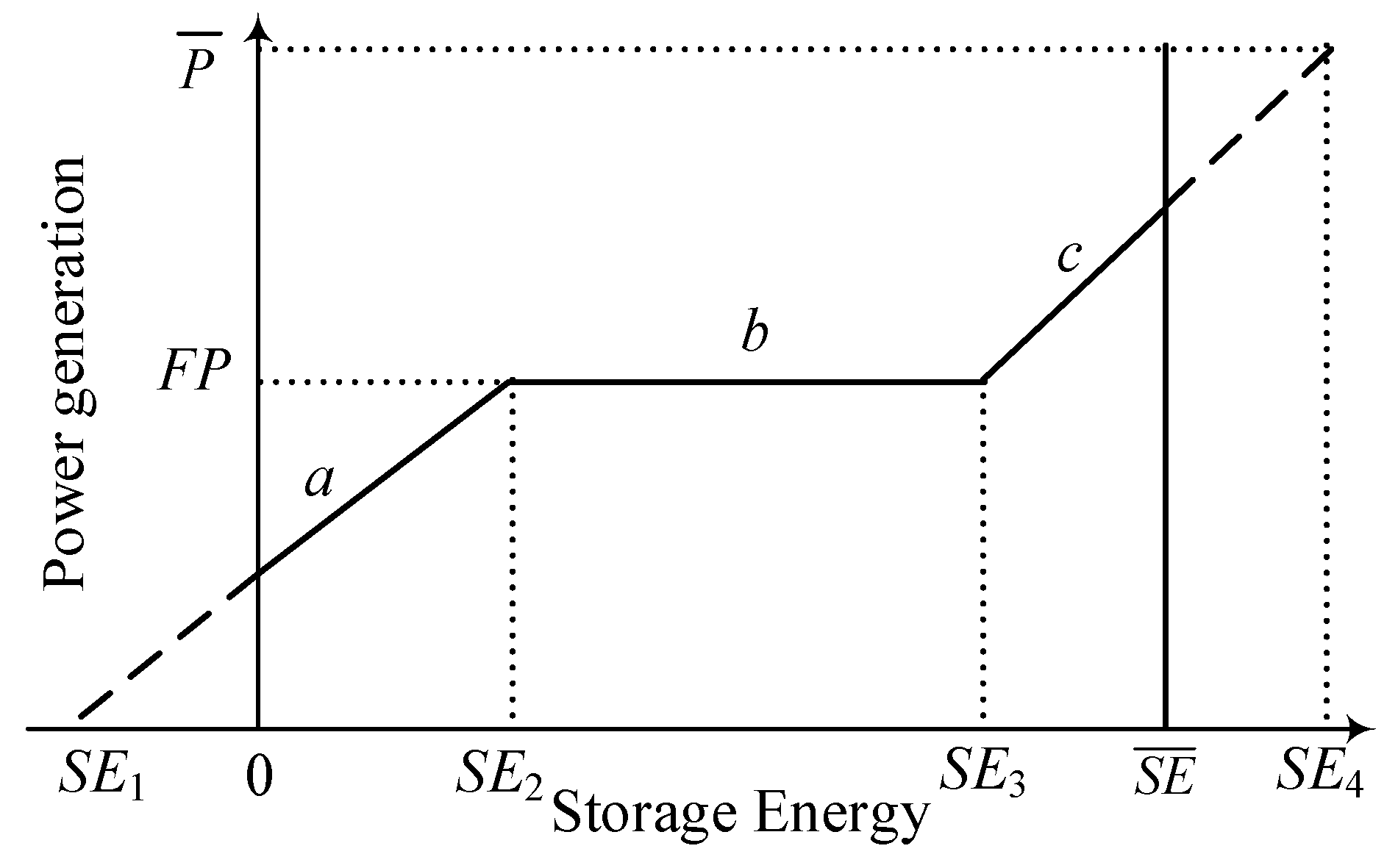
2.1. Operation Rule for Large-Scale Hydropower System

The monthly rule curves of cascade reservoirs and the cascade decision allocation method of cascade reservoirs constitute the operating rules adopted in this paper. The energy storage of the cascade reservoir system is usually adopted as the state variable that determines the whole cascade decision [17,25]. In this paper, the storage energy for a hydropower system is computed using Equation (1),

$$S{E}^t={\displaystyle \sum }_{m=1}^M\left\{e_m{w}_m^t{H}_m\left[g\left(w_m^t,{\underset{\_}{s}}_m^t\right)\right]+w_m^t{\displaystyle \sum }_{k=m+1}^M{e}_k{H}_k\left[z_k\left(s_k^t\right)\right]\right\}$$

(1)

where $S{E}^t$ is the initial storage energy at period t for reservoir m, $e_m$ is the efficiency of power generation, $w_m^t$ is the initial active storage at the period t, $H_m( )$ is a function to calculate power generating head under a given reservoir level, $g\left(w_m^t,{\underset{\_}{s}}_m^t\right)$ is a function to calculate the center of gravity of the water volume $w_m^t$ above ${\underset{\_}{s}}_m^t$, $z_k( )$ is a function to calculate the initial reservoir level, and $s_k^t$ is the initial reservoir storage.

Figure 1 shows the three-segment rule curve which is usually used for reservoir operation. Firm power is the guaranteed power provided by the hydropower plant even under adverse conditions. Line a is the segment where power generation is smaller than firm power, line b is the segment where power generation is at firm power, and line c is the segment where power generation is larger than firm power. In Figure 1, the monthly varying storage energy values of $S{E}_{t,i}$, t = 1:12 and i = 1:4, are to be optimized.

The cascade power generation decision made by using the rule curve needs to be allocated to each reservoir. A power allocation method that adopts a simplified Sheer rule [26] to maximize the objective $z^{\prime t}={\sum }_{m=1}^M{e}_m\left[{\overline{H^{″}}}_m\left(S_{m,f}^t\right){\overline{Q}}_m^t\right]$ was proposed by Wu et al. [27]. By giving the ending storage of $S_{m,f}^t$ at current period, ${\overline{H^{″}}}_m\left(S_{m,f}^t\right)$ is the expected release-weighted hydropower head from the end of the current time step t until reservoir refill or emptying. ${\overline{Q}}_m^t$ is the expected turbine release volume from the end of the current period t until reservoir refill or emptying. In the power allocation method, downstream reservoir j captures the release of upstream reservoir m and is set to be the decision variable $T_{m,j}^t$. By increasing or decreasing one or several $T_{m,j}^t$ in turn of $\frac{\partial {z^{\prime }}^t}{\partial E{T}_{m,j}^t}=\frac{\partial {z^{\prime }}^t}{\partial T_{m,j}^t}\frac{\partial T_{m,j}^t}{\partial E{T}_{m,j}^t}$, the total cascade power decision is allocated. The total energy $E{T}_{m,j}^t$ is generated by $T_{m,j}^t$ at reservoirs from m to j-1. The power allocation method should satisfy the minimum release constraints of the reservoirs as much as possible. The values of ${\overline{H^{″}}}_m\left(S_{m,f}^t\right)$ and ${\overline{Q}}_m^t$ vary with operation rules and can be approximately estimated by using simulation results from an individual reservoir operation rule before optimizing cascade operation rules, and in most cases, this error may not affect the sorting of $T_{m,j}^t$.

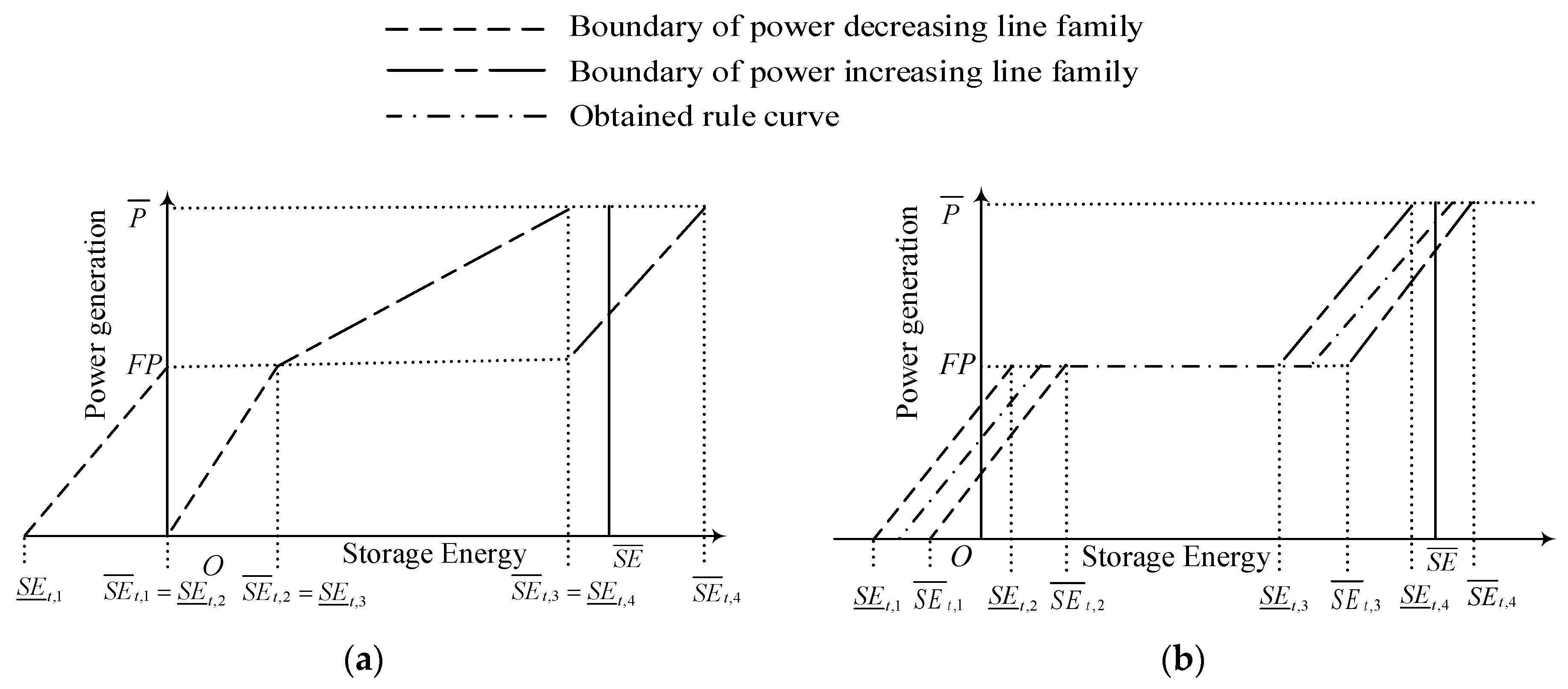
2.2. Optimization Model for Operation Rule

For each cascade hydropower station that belongs to a power generation agent, the traditional operation mode is energy maximization. Noting the operation rule $R$, the model is formulated as follows:

$$\underset{R}{\mathit{max}} F={\displaystyle \sum }_{m=1}^M{\displaystyle \sum }_{t=1}^T{E}_m^t$$

(2)

$$E_m^t=e_m{q}_m^t\left[\left(z_m^t+z_m^{t+1}\right)/2-z{d}_m^t\right]$$

(3)

$$s_m^t+Q_m^t-r_m^t=s_m^{t+1}$$

(4)

$${\underset{\_}{s}}_m^t\le s_m^t\le {\overline{s}}_m^t$$

(5)

$$p_m^t\le {\overline{p}}_m^t$$

(6)

$${\underset{\_}{r}}_m^t\le r_m^t$$

(7)

$${\displaystyle \sum }_{m=1}^M{p}_m^t\ge \underset{\_}{P}$$

(8)

where m and t are sequence numbers of reservoirs and periods, $F$ is the objective function of energy generation in simulation horizon, T is the number of periods in simulation horizon, and the time step is the month, $E_m^t$ is the energy generation, $q_m^t$ is the turbine release volume, $e_m$ is the efficiency of power generation, $z_m^t$ is the initial reservoir level, a function of initial reservoir storage $s_m^t$, $z{d}_m^t$ is the average tailwater level, local inflow and arriving outflow of upstream reservoirs compose the water inflow volume $Q_m^t$, turbine release volume $q_m^t$ and water spillage $d_m^t$ compose the reservoir release volume $r_m^t$, ${\underset{\_}{s}}_m^t$ and ${\overline{s}}_m^t$ are the lower and upper bound for reservoir storage respectively, ${\underset{\_}{r}}_m^t$ is the minimum water release volume, $E_m^t=p_m^t{h}^t$, $p_m^t$ is the power generation, $h^t$ is the number of the period hour, the installed capacity often is the maximum power ${\overline{p}}_m^t$, and $\underset{\_}{P}$ is firm power for the hydropower system.

The model means optimizing the operation rule R to obtain the maximum energy generation in simulation by using historical inflow data with the consideration of constraints (Equations (2)–(8)).

2.3. GA-Based Simulation-Optimization Method for Operation Rule

The optimization model for operation rules can be solved by GA. GA has been widely used to solve reservoir optimal operation models. GA can optimize the operation schedules [28,29,30,31] or operation rules [32,33]. In the GA of this paper, the objective function or fitness value of each individual in GA is obtained by simulation with $S{E}_{t,i}$, t = 1:12 and i = 1:4 as variables. Due to the uncertainty of reservoir inflow, the firm power constraint (Equation (8)) of the whole system cannot be satisfied at all simulation periods. Some models addressed the firm power constraint as a chance constraint, and it needs to be satisfied at certain probabilities [34,35]. The constraint can also be addressed by using the penalty function on the period shortage amount, and the penalty function can be linear and quadratic. In hydropower operation in some power systems, the managers are more willing to accept a smaller shortage in more periods, instead of accepting a larger shortage in fewer periods. Therefore, this paper adopts the quadratic penalty function on a firm power shortage. For a similar reason, the penalty function of the minimum reservoir release constraint is also quadratic.

Considering the constraints of firm power and minimum reservoir release, the fitness function is ${\sum }_{t=1}^T{\sum }_{m=1}^M{E}_m^t-{\sum }_{t=1}^{T}a{\left[\mathit{min}\left({\sum }_{m=1}^M{p}_m^t-\underset{\_}{P},0\right)\right]}^2-{\sum }_{t=1}^T{\sum }_{m=1}^{M}b{\left[\mathit{min}\left(f_m^t-{\underset{\_}{f}}_m^t,0\right)\right]}^2$, a and b are penalty coefficients for firm power and minimum release respectively, and $f_m^t$ and ${\underset{\_}{f}}_m^t$ are the rate of release flow and its minimum constraint, according to $r_m^t$ and ${\underset{\_}{r}}_m^t$, respectively.

A single solution to the problem in GA terminology is called a chromosome. In this paper, the variables of $S{E}_{t,i}$, t = 1:12 and i = 1:4, compose the chromosomes by using real number encoding [36]. The adopted GA procedure generates a population of size n randomly at the beginning. Through crossover and mutation, an offspring population of equal size n is created. The two-point crossover operator and non-uniform mutation operator [37] are used. Then, a population of size 2 n is formed by combining the parents and the offspring. The members of this new population are sorted in descending order of fitness, and the n strongest individuals are selected as the next-generation population. The evolutionary process is repeated for a preset maximum generation, or until the optimal fitness value is not changed in some continuous generations.

Because there are 48 variables to be determined by GA, and the computation of fitness values is very time consuming, the population size and evolution generation cannot be too large. Therefore, it is impossible to optimize the whole feasible domain in a limited time. In the meantime, the feasible region of $S{E}_{t,i}$ is constrained by the relation of $S{E}_{t,i}\le S{E}_{t,i+1}$, i = 1:3, which means that there are many infeasible solutions in the computation process of GA when defining $S{E}_{t,i}$, i = 1:4 on ${\underset{\_}{SE}}_t\le S{E}_{t,i}\le {\overline{SE}}_t$. In order to obtain rule curves at an acceptable time, and avoid the influence of infeasible solutions, the feasible region of $S{E}_{t,i}$ can be set in a certain region of $\left[{\underset{\_}{SE}}_{t,i},{\overline{SE}}_{t,i}\right]$, here, ${\underset{\_}{S}}_{t,i}$ and ${\overline{S}}_{t,i}$ are the lower and upper bound of $S{E}_{t,i}$, respectively. The boundary satisfies ${\overline{SE}}_{t,i}\le {\underset{\_}{SE}}_{t,i+1}$, i = 1:3. It means that the region of $\left[{\underset{\_}{SE}}_t,{\overline{SE}}_t\right]$ is divided into 4 sub-regions, and $S{E}_{t,i}$ is defined in each sub-region. By dividing $\left[{\underset{\_}{SE}}_t,{\overline{SE}}_t\right]$, the feasible region of each variable is significantly reduced, which is beneficial to efficiency. However, if the feasible region is not well defined, the risk of obtaining poor solutions is increased.

Because of the complexity of the model, GA cannot obtain the global optimal solution, but can only get the sub-optimal solution. In order to reduce the influence of feasible region division, multiple GA with the different feasible region can be used to solve the model according to the result of the former GA, and the solution of the former GA can be regarded as an individual of the initial population. Figure 2 shows an example of a feasible region reduction. In the first step, as shown in Figure 2a, the lower and upper bounds of the adjacent variable are set equal to ${\overline{SE}}_{t,1}={\underset{\_}{SE}}_{t,2}$, ${\overline{SE}}_{t,2}={\underset{\_}{SE}}_{t,3}$ and ${\overline{SE}}_{t,3}={\underset{\_}{SE}}_{t,4}$, and the boundary values are set according to experiences. Any line starting from coordinate ($S{E}_{t,1}$, 0) and ending in ($S{E}_{t,2}$, FP) denotes a power decreasing line, any line starting from coordinate ($S{E}_{t,3}$, FP) and ending in ($S{E}_{t,4}$, $\overline{P}$) denotes a power increasing line, and the line connecting ($S{E}_{t,2}$, FP) and ($S{E}_{t,3}$, FP) is the firm power line. So, the feasible region of power decreasing line and power increasing line can be denoted as in Figure 2a. After using GA to divide the rule curve according to the feasible region, the feasible region can be updated as shown in Figure 2b, and a new round of optimization can be carried out in the new feasible region. The new feasible region can be smaller than the initial feasible region, or it can include regions that are not in the initial feasible region. For example, when $S{E}_{t,i}={\overline{SE}}_{t,i}$ in the obtained rule curve, the upper bound can be updated to ${\overline{SE}}_{t,i}={\overline{SE}}_{t,i}+\mathsf{\Delta }$. When $S{E}_{t,i}={\underset{\_}{SE}}_{t,i}$ in the obtained rule curve, the lower bound can be updated to ${\underset{\_}{SE}}_{t,i}={\underset{\_}{SE}}_{t,i}-\Delta$. Here, $\Delta$ is a step length of renewing the feasible region.

Obviously, it may be much more difficult to optimize the rule curve in the initial feasible region as shown in Figure 2a than in a smaller feasible region as shown in Figure 2b. In addition, it is difficult to set the initial boundary of variables, which may lead to the poor performance of the obtained rule curve.

2.4. Derive Initial Operation Rule Using an Aggregated SSDP

According to the former analysis, a well-derived initial solution helps set initial feasible regions and is important to both solving efficiency and quality. In common SSDP, reservoir storage is often used as a state variable. However, the dimension problem limits the application of SSDP in a large-scale reservoir system. In this paper, an aggregated SSDP is used to obtain the initial solution. Some aggregation-disaggregation approaches exist for reservoir operations [4,5,6,7], while the aggregated SSDP used in this paper need not accurately solve the optimal operation model, for the aim of the aggregated SSDP is only used to obtain an initial solution, and the final operation rule can be improved through simulation-optimization. To aggregate a large-scale hydropower system, the storage energy, as in Equation (1), is used as a state variable, and the power generation of the whole system is the decision variable. The storage energy can only approximately describe the state of a hydropower system, meaning that different reservoir level combinations may have the same value of storage energy. Assuming that all reservoirs in the system store and discharge water synchronously, and the ratios of reservoir storage to its upper bound of the period are the same. Then, a hydropower system is operated like one reservoir. Using N yearly inflow scenarios, and assuming that the probability of each inflow scenario is the same and independent of inflow that happened in the past, the recursive functions of the aggregated SSDP are Equations (9)–(11):

$$\underset{P^t}{max} F^t\left(S{E}^t\right)={\displaystyle \sum }_{n=1}^N\frac{1}{N}{f}^{t,n}\left(S{E}^t\right)$$

(9)

$$f^{t,n}\left(S{E}^t\right)=\left[B^{t,n}\left(S{E}^t,P^t\right)+g^{t+1,n}\left(S{E}^{t+1}\right)\right]$$

(10)

$$g^{t+1,n}\left(S{E}^{t+1}\right)=\{\begin{array}{l}{f}^{t+1,n}\left(S{E}^{t+1}\right) t\ne T0\\ \frac{1}{N}{\displaystyle {\displaystyle \sum }_{n0=1}^N}{f}^{t+1,n0}\left(S{E}^{t+1}\right) t=T0\end{array}$$

(11)

where at period t, $F^t\left(S{E}^t\right)$ is the objective function at state $S{E}^t, f^{t,n}\left(S{E}^t\right)$ is the objective function for inflow scenario n, $B^{t,n}\left(S{E}^t,P^t\right)$ is benefit function at period t for inflow scenario n, $g^{t+1,n}\left(S{E}^{t+1}\right)$ is future value function for inflow scenario n, and T0 is the period number in a year.

In the solution using the SSDP, there is an aggregation-disaggregation algorithm. In the aggregating computation, given a storage energy state $S{E}^t$ of a cascade system at period t, the aggregation procedure is to search for a ratio $\gamma =\left(s_m^t-{\underset{\_}{s}}_m^t\right)/\left({\overline{s}}_m^t-{\underset{\_}{s}}_m^t\right)$ for all reservoirs m, obtaining the storage energy $S{E}^t$ using Equation (1). In the disaggregating computation, given period initial reservoir storage value, total power generating decision, and inflow, the decomposition procedure is to search for a ratio $\gamma =\left(s_m^{t+1}-{\underset{\_}{s}}_m^{t+1}\right)/\left({\overline{s}}_m^{t+1}-{\underset{\_}{s}}_m^{t+1}\right)$ for all reservoirs m. The power decision can be obtained when all the reservoirs try to operate for the ending storage.

In the benefit function, the system firm power can be reflected by using a penalty term, but the reservoir minimum release cannot be included. Since the reservoirs are assumed to store and discharge water synchronously, the minimum release cannot be satisfied for all reservoirs unless the reservoir storage drawing down extents to satisfy the minimum release of all reservoirs are the same. Therefore, the minimum release constraint is ignored when deriving the initial rule, and $B^{t,n}\left(S{E}^t,P^t\right)={\sum }_{m=1}^M{E}_m^t-a{\left[\mathit{min}\left({\sum }_{m=1}^M{p}_m^t-\underset{\_}{P},0\right)\right]}^2$.

Equations (9)–(11) define a recursive computation of periodic Markov processes in an infinite horizon, where one cycle corresponds to one year. The SSDP solution needs to obtain an optimal decision at each state from the last period T to the first period 1 backward in a year. This process is repeated until decisions converge in all periods and all states. At the beginning of each iteration, the future value function of period T is replaced by the value function of period 1 of the last iteration. At each station, the optimal solution is obtained through the search after traversing [38]. In the traversing stage, an optimal solution is selected from the discrete decision points. In the searching stage, a better stage solution is obtained near the optimal solution in traversing.

3. Case Study

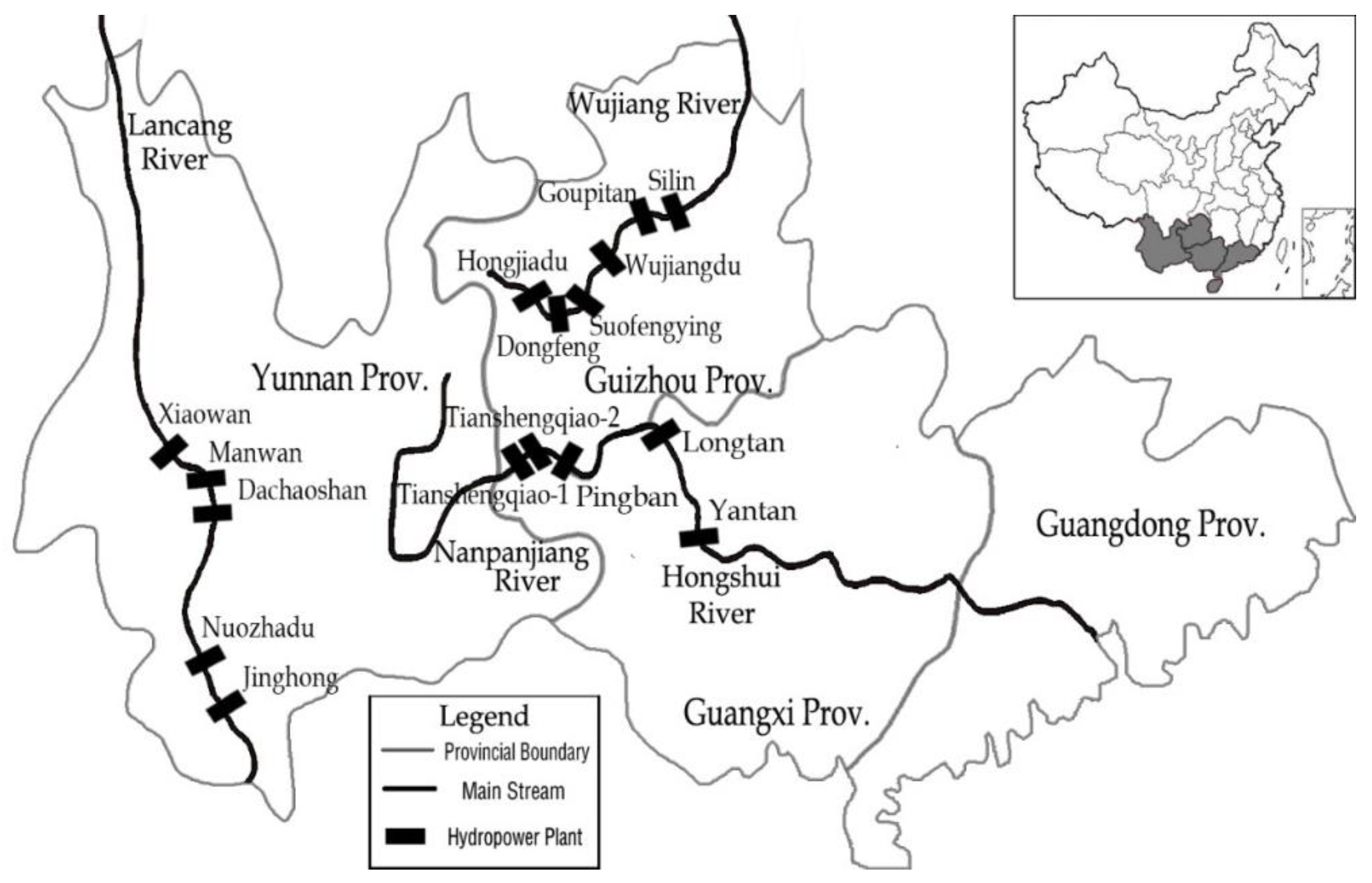
3.1. Introduction to the Engineering Background

In China, the Hongshui River system, the Wu River system, and the Lancang River system are important power sources of west–east transmission [39]. These three cascaded basins compose the studied system. Hongshui River ranks second in China for runoff volume and is the upper reach of Pearl River. It originates from the Nanpan River in Yunnan Province, after the confluence with the Beipan River in Guizhou Province, which is known as the Hongshui River. The Wu River is the largest tributary on the south of the Yangtse River. The Wu River cascaded system is located on the main stem in Guizhou Province. The Lancang River, known outside China as the Mekong River, is an international river. The Lancang River cascaded system is located on the main stem in Yunnan Province. June to September is the main flood season, while January to April is the main dry season. To make long-term operating plans, the control and dispatching centers negotiate with the cascade operating centers. The energy prices are considered constant in all periods for all reservoirs, and the objective or constraints for power grid demands usually use total energy or power. Figure 3 shows the hydropower system, with reservoir characteristics in

Table 1. Characteristics of the studied hydropower system.

Hongshui River			Lancang River			Wu River
Reservoir	Installed Capacity (MW)	Beneficial Storage (108 m3)	Reservoir	Installed Capacity (MW)	Beneficial Storage (108 m3)	Reservoir	Installed Capacity (MW)	Beneficial Storage (108 m3)
Tianshengqiao-1	1200	57.95	Xiaowan	4200	98.77	Hongjiadu	600	33.60
Tianshengqiao-2	1320	0.08	Manwan	1670	2.57	Dongfeng	695	4.90
Pingban	405	0.27	Dachaoshan	1350	3.70	Suofengying	600	0.67
Longtan	4900	111.49	Nuozhadu	5850	113.35	Wujiangdu	1250	13.60
Yantan	1210	10.50	Jinghong	1750	3.09	Goupitan	3000	29.02
						Silin	1050	3.18
Total	9035		Total	14,820		Total	7195

The storage abilities of the 6 aggregated reservoirs in bold are considered, with the other reservoirs considered to be runoff from the river.

, the storage abilities of the aggregated 6 reservoirs are considered, with the other reservoirs considered to be runoff from the river. In the simulation, inflow data from 1953–2008 are used. Set the firm power of the three cascade systems at 13,000 MW, and the penalty coefficients a and b in the penalty function are both 10⁵.

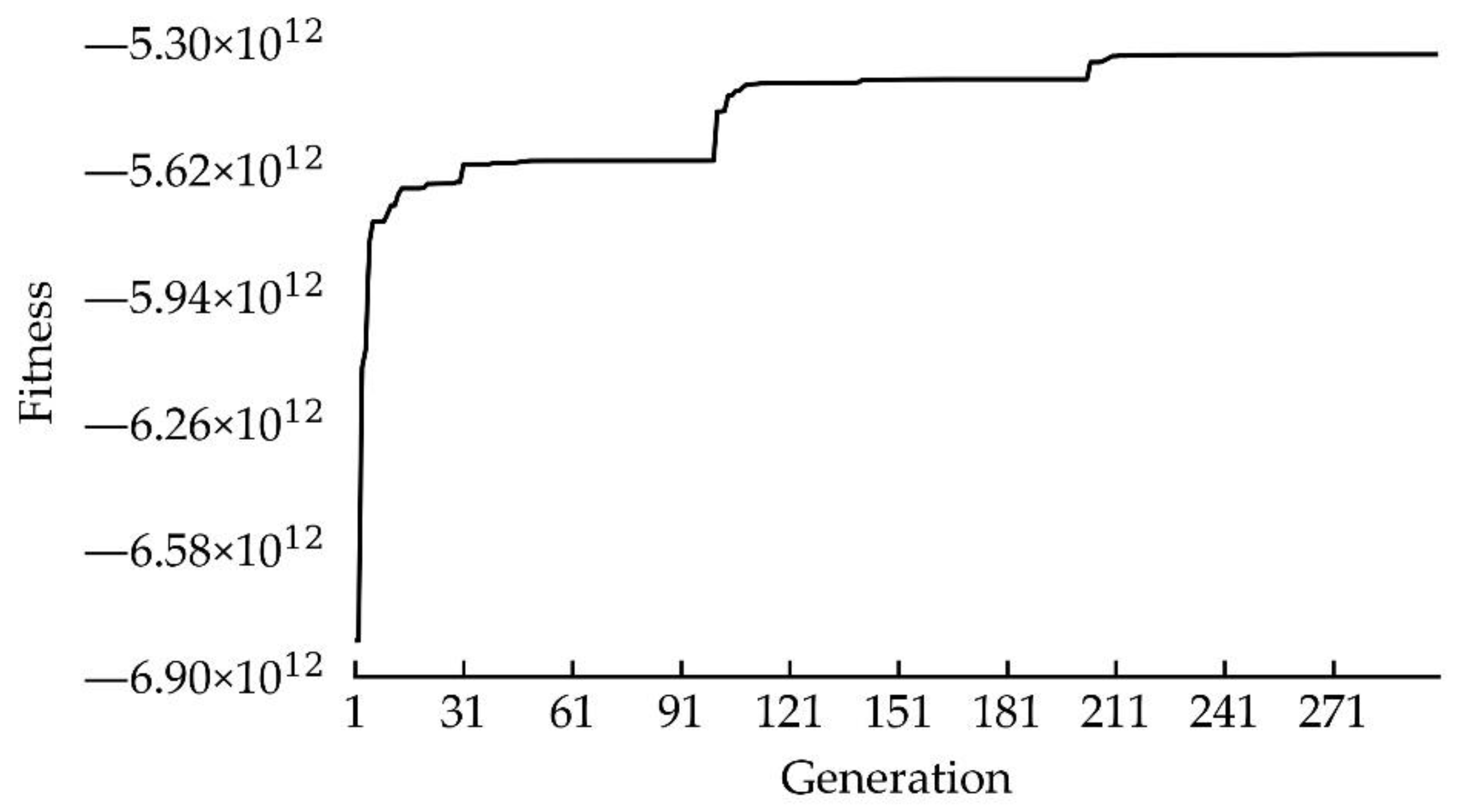
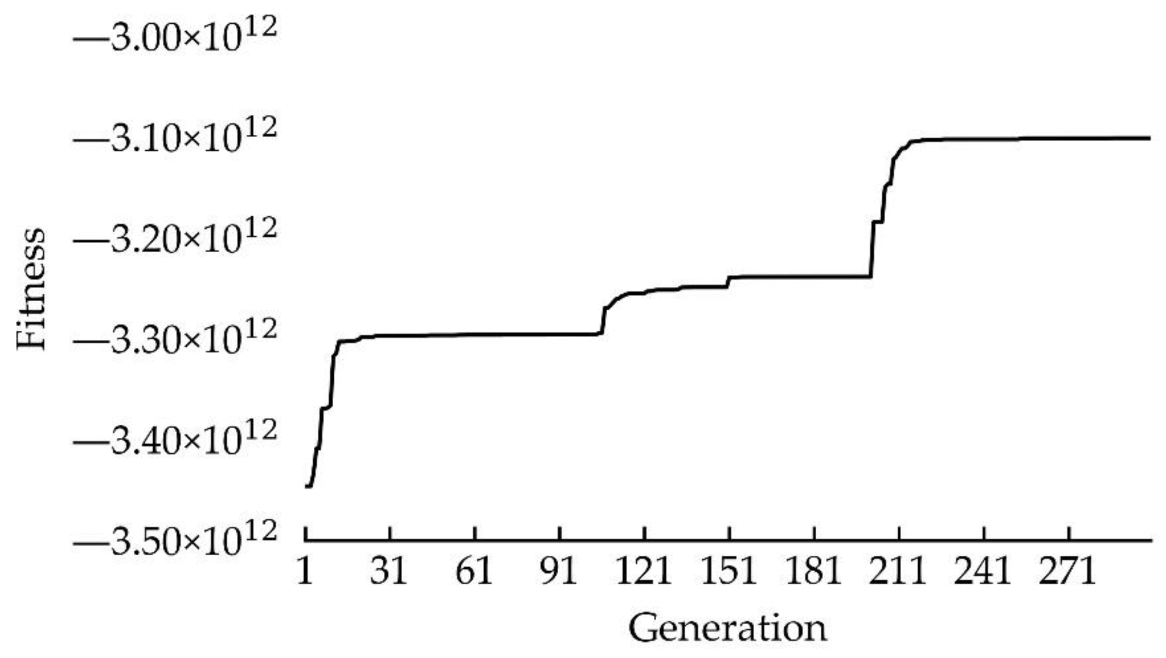
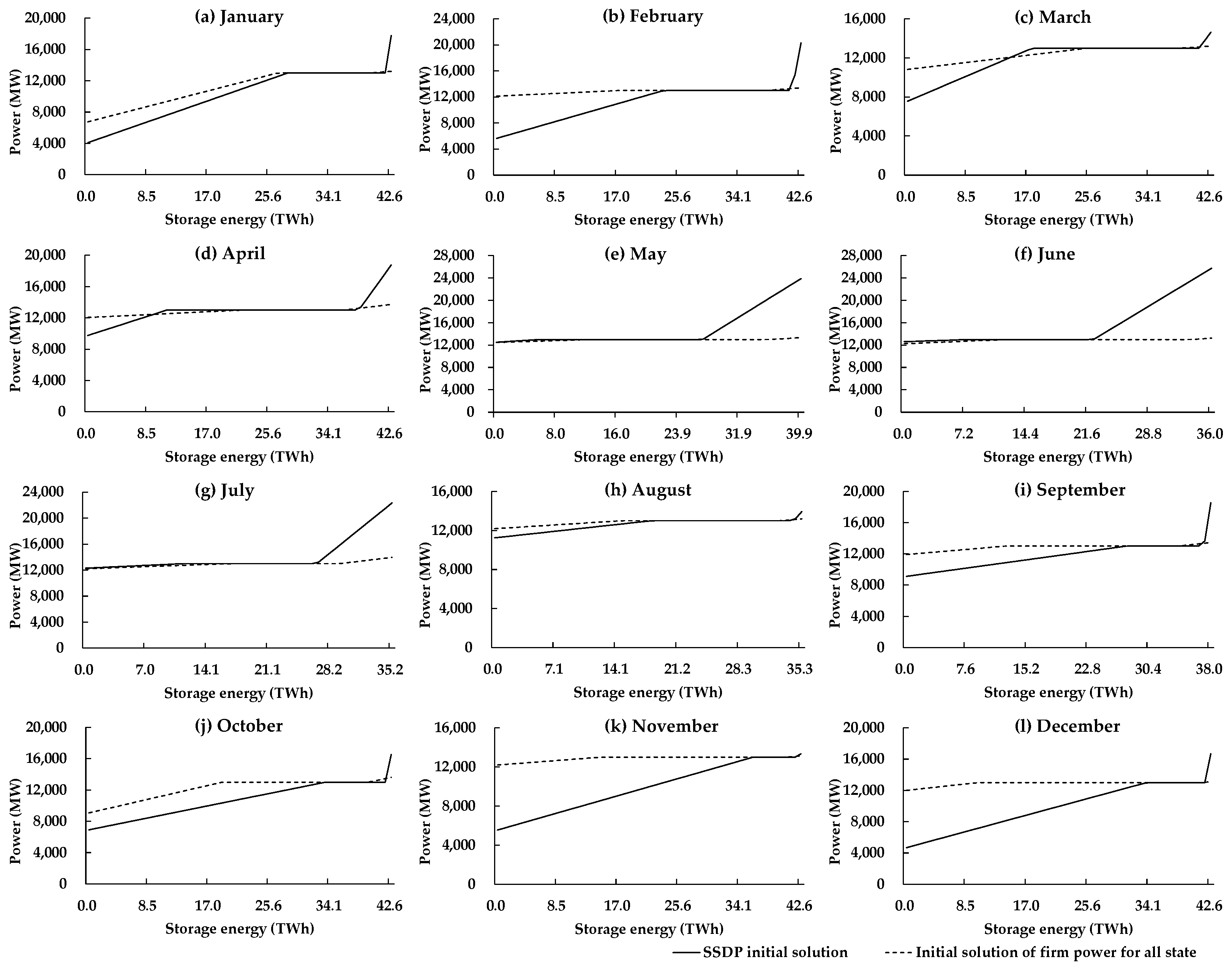
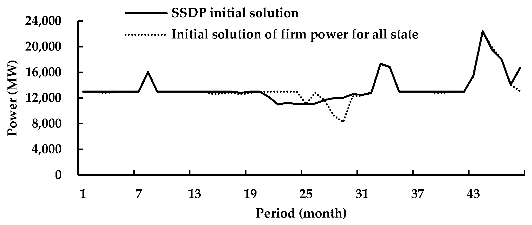
3.2. Numerical Results

By using the traditional one-stage simulation-optimization method based on GA, there is no method to obtain an initial solution. So, one can easily take the solution of firm power for all storage energy as an initial solution. Therefore, at first, the initial solution is set as the firm power for all storage energy at all periods, and it is an individual in the initial population of GA. In Figure 1, the initial feasible region of SE₁, SE₂, SE₃, and SE₄ are set at $\left[-10\overline{SE},0\right]$, $\left[0,0.8\overline{SE}\right]$, $\left[0.8\overline{SE},\overline{SE}\right],$ and $\left[\overline{SE},11\overline{SE}\right]$, respectively. The GA is run three times. After each run, the feasible region of SE₁, SE₂, SE₃, and SE₄ are reduced to $\left[S{E}_i-c\overline{SE},S{E}_i+c\overline{SE}\right]$, i = 1:4, c is a ratio number, and 0.1 and 0.05 are used after the first and the second GA run, respectively. If the feasible regions for two adjacent $S{E}_i$ intersect, they will be reduced by half of the intersected part. In each GA run, the population size P is set to 100, and the maximum evolutionary generation G is also set to 100. The operation rule obtained by the one-stage method is denoted as rule 1.

Figure 4 shows the process of evolution. There are three 100-generation evolutionary segments, each of them resulted from a GA run. In the first round of the GA run, the fitness value of the first several generations grows very fast, while it grows slowly after 30 generations, which means that the convergence is very fast. In the latter two rounds of the GA procedure, the fitness value increases slowly after 15 generations, indicating that the convergence speed is faster than the first round because the feasible region of the latter two rounds of the GA procedure is smaller than the first round.

Table 2. Simulation results of operation rules obtained by these two methods.

Solution	Energy Generation (TWh)	Total Firm Power Shortage (MW)	Maximum Firm Power Shortage (MW)	Objective Function
All firm power rules	7339.4	18,652	7993	−1.01 × 1013
SSDP rule	7343.0	27,318	2449	−3.59 × 1012
Rule 1	7344.5	41,293	4761	−5.33 × 1012
Rule 2	7344.5	26,442	2016	−3.10 × 1012

shows the simulation result. The fitness value has increased from −1.01 × 10¹³ to −5.33 × 10¹² through the three GA runs, and the increasing percentage is about 47.2%. Because the population size and evolution generations are too small to obtain a global optimal solution of the model, in the next case, a fast obtained solution will be used as the initial individual. All the fitness values are negative because the value of the penalty term for firm power is much larger than the energy generation.

Then, by using the proposed two-stage method, the initial solution is set as the result of the SSDP. The operation rule is optimized using the same settings and computing process as the previous case with only the initial solution different. In the SSDP, the 51 discretized storage energy of each period is used. The operation rule obtained by the two-stage method is denoted as rule 2. Table 2 shows the simulation results. The fitness value has increased from −3.59 × 10¹² to −3.10 × 10¹² through the three GA runs, and the increasing percentage is about 13.6%. Figure 5 shows the process of evolution. Comparing to the evolutionary process by using the one-stage method, the extent of fitness improvement is small, while the value of the objective function for rule 2 is much larger than rule 1, and the firm power shortage is much smaller. So, the quality of rule 2 is better than rule 1 due to a better initial solution.

Figure 6 shows the operation rules obtained by using both methods. In most months, it is obvious that the power generation decision of rule 2 for low storage energy is smaller than that of rule 1. The GA only obtains the local optimal solution near the initial solution. From the initial solution of firm power for all states, curves of rule 1 are closer to the firm power than rule 2. While in the SSDP model, a quadratic penalty function is adopted to solve the firm power constraint. So, in rule 2, there are power decreasing regions where the power decision is smaller than firm power and decreased with decreasing storage energy, in all months besides May, June, and July. By using the two-stage optimization method with the SSDP initial solution, the power decreasing regions are maintained.

The difference between the objective function values using these two operation rules is mainly due to the shortage extent in some dry season months. Figure 7 shows an example of simulation difference in several years. Using rule 1, the periods of firm power shortage are shorter than using rule 2, and the shortage extent is larger. It is because the power decreasing regions of rule 2 are much larger than rule 1. Therefore, using rule 2, the hydropower system reduces power generation earlier than using rule 1, and the shortage is allocated to more periods than when using rule 1. The penalty function of firm power is quadratic, which means that the same amount of power shortage occurring in more periods is better than that occurring in fewer periods. Without a good initial solution, the result of the traditional one-stage simulation-optimization method based on GA does not fully reflect the intention, while the two-stage method does.

In a personal computer with four 2.8 GHz central processing units, the computation time for each GA run is about 80 h, while the SSDP is about 3 h. So, the total computation time for obtaining the operation rule by using the proposed two-stage method is about 243 h. This is acceptable for the long-term operation of reservoirs. For the one-stage method without an initial solution, a much larger population size and evolutionary generation are needed to obtain a similar performance solution, and the computation time will increase a lot, which is beyond the acceptable extent.

4. Conclusions

In this paper, a two-stage method was proposed to derive operation rules for a large-scale hydropower system. In the first stage, an initial solution is obtained by using an aggregated SSDP. In the second stage, a simulation-optimization model is solved by using several rounds of the GA procedure, the feasible region is reduced after each round of GA, and the initial solution obtained in the first stage is used as an initial individual in the first round of GA. Due to the complexity of operation in large-scale hydropower reservoirs, the dimension problem limits the adoption of common SSDP in a large-scale reservoir system, and the conventional simulation-optimization methods can only obtain a local solution in most cases. The combination method is novel and can improve the quality of the solution without much of an increase in computing time.

The proposed method was used for the operation of three cascaded hydropower reservoirs in Southwest China to test the validity and practicability. The result showed that the fast convergent GA can only obtain a solution near the initial solution, and the global optimization ability cannot be fully exerted. Therefore, a good initial solution is crucial to the result, and the aggregated SSDP is an appropriate method to obtain an initial solution. Using a good initial solution, the proposed two-stage method obtained a much better solution than the traditional single-stage method. Without the initial solution, much larger population size and evolutionary generation are needed to obtain a similar performance solution, and the computation time will increase a lot, which is beyond the acceptable extent.

Since large amounts of complex cascade hydropower systems have been formed in China, it is difficult for a traditional algorithm to derive high-quality operation rules within an acceptable time. From the detailed comparison of numerical results, it can be seen that compared with the traditional one-stage simulation-optimization method based on GA, this combination method can obtain higher-quality solutions without increasing the solution time. We believe that the method proposed in this paper is of great significance and could provide a reference to derive operation rules for a large-scale hydropower system.

References

1. Feng, Z.K.; Niu, W.J.; Cheng, X.; Wang, J.Y.; Wang, S.; Song, Z.G. An effective three-stage hybrid optimization method for source-network-load power generation of cascade hydropower reservoirs serving multiple interconnected power grids. J. Clean. Prod. 2020, 246, 119035. [Google Scholar] [CrossRef]
2. Lei, X.-H.; Tan, Q.-F.; Wang, X.; Wang, H.; Wen, X.; Wang, C.; Zhang, J.-W. Stochastic optimal operation of reservoirs based on copula functions. J. Hydrol. 2018, 557, 265–275. [Google Scholar] [CrossRef]
3. Côté, P.; Arsenault, R. Efficient Implementation of Sampling Stochastic Dynamic Programming Algorithm for Multireservoir Management in the Hydropower Sector. J. Water Resour. Plan. Manag. 2019, 145. [Google Scholar] [CrossRef]
4. Turgeon, A. Optimal operation of multireservoir power systems with stochastic inflows. Water Resour. Res. 1980, 16, 275–283. [Google Scholar] [CrossRef]
5. Turgeon, A.C. Raymond An aggregation-disaggregation approach to long-term reservoir management. Water Resour. Res. 1998, 34, 3585–3594. [Google Scholar] [CrossRef]
6. Tan, Q.-F.; Wang, X.; Wang, H.; Wang, C.; Lei, X.-H.; Xiong, Y.-S.; Zhang, W. Derivation of optimal joint operating rules for multi-purpose multi-reservoir water-supply system. J. Hydrol. 2017, 551, 253–264. [Google Scholar] [CrossRef]
7. Pan, Z.; Chen, L.; Teng, X. Research on joint flood control operation rule of parallel reservoir group based on aggregation–decomposition method. J. Hydrol. 2020, 590. [Google Scholar] [CrossRef]
8. Helseth, A.; Braaten, H. Efficient Parallelization of the Stochastic Dual Dynamic Programming Algorithm Applied to Hydropower Scheduling. Energies 2015, 8, 14287–14297. [Google Scholar] [CrossRef] [Green Version]
9. Raso, L.; Chiavico, M.; Dorchies, D. Optimal and Centralized Reservoir Management for Drought and Flood Protection on the Upper Seine–Aube River System Using Stochastic Dual Dynamic Programming. J. Water Resour. Plan. Manag. 2019, 145. [Google Scholar] [CrossRef] [Green Version]
10. Yeh, W.W.G. Reservoir management and operations models: A state-of-the-art review. Water Resour. Res. 1985, 21, 1797–1818. [Google Scholar] [CrossRef]
11. Labadie, J.W. Optimal operation of multireservoir systems: State-of-the-art review. J. Water Resour. Plan. Manag. 2004, 130, 93–111. [Google Scholar] [CrossRef]
12. Powell, W.B. Approximate Dynamic Programming: Solving the Curses of Dimensionality; John Wiley & Sons: Hoboken, NJ, USA, 2007; Volume 703. [Google Scholar]
13. Giuliani, M.; Castelletti, A.; Pianosi, F.; Mason, E.; Reed, P.M. Curses, Tradeoffs, and Scalable Management: Advancing Evolutionary Multiobjective Direct Policy Search to Improve Water Reservoir Operations. J. Water Resour. Plan. Manag. 2016, 142, 04015050. [Google Scholar] [CrossRef] [Green Version]
14. Lund, J.R.; Ferreira, I. Operating rule optimization for Missouri River reservoir system. J. Water Resour. Plan. Manag. Asce 1996, 122, 287–295. [Google Scholar] [CrossRef]
15. Ji, C.M.; Zhou, T.; Huang, H.T. Operating Rules Derivation of Jinsha Reservoirs System with Parameter Calibrated Support Vector Regression. Water Resour. Manag. 2014, 28, 2435–2451. [Google Scholar] [CrossRef]
16. Jiang, Z.; Song, P.; Liao, X. Optimization of Year-End Water Level of Multi-Year Regulating Reservoir in Cascade Hydropower System Considering the Inflow Frequency Difference. Energies 2020, 13, 5345. [Google Scholar] [CrossRef]
17. Liu, P.; Guo, S.L.; Xu, X.W.; Chen, J.H. Derivation of Aggregation-Based Joint Operating Rule Curves for Cascade Hydropower Reservoirs. Water Resour. Manag. 2011, 25, 3177–3200. [Google Scholar] [CrossRef]
18. Koutsoyiannis, D.E. Athanasia Evaluation of the parameterization-simulation-optimization approach for the control of reservoir systems. Water Resour. Res. 2003, 39. [Google Scholar] [CrossRef] [Green Version]
19. Rani, D.; Moreira, M.M. Simulation–Optimization Modeling: A Survey and Potential Application in Reservoir Systems Operation. Water Resour. Manag. 2009, 24, 1107–1138. [Google Scholar] [CrossRef] [Green Version]
20. Oliveira, R.; Loucks, D.P. Operating rules for multireservoir systems. Water Resour. Res. 1997, 33, 839–852. [Google Scholar] [CrossRef]
21. Chang, L.C.; Chang, F.J.; Wang, K.W.; Dai, S.Y. Constrained genetic algorithms for optimizing multi-use reservoir operation. J. Hydrol. 2010, 390, 66–74. [Google Scholar] [CrossRef]
22. Liu, X.; Guo, S.; Liu, P.; Chen, L.; Li, X. Deriving Optimal Refill Rules for Multi-Purpose Reservoir Operation. Water Resour. Manag. 2010, 25, 431–448. [Google Scholar] [CrossRef]
23. Taghian, M.; Rosbjerg, D.; Haghighi, A.; Madsen, H. Optimization of Conventional Rule Curves Coupled with Hedging Rules for Reservoir Operation. J. Water Resour. Plan. Manag. 2014, 140, 693–698. [Google Scholar] [CrossRef]
24. Latorre, J.M.; Cerisola, S.; Ramos, A.; Perea, A.; Bellido, R. Coordinated Hydropower Plant Simulation for Multireservoir Systems. J. Water Resour. Plan. Manag. 2014, 140, 216–227. [Google Scholar] [CrossRef]
25. Jiang, Z.Q.; Qin, H.; Ji, C.M.; Hu, D.C.; Zhou, J.Z. Effect Analysis of Operation Stage Difference on Energy Storage Operation Chart of Cascade Reservoirs. Water Resour. Manag. 2019, 33, 1349–1365. [Google Scholar] [CrossRef]
26. Lund, J.R. Derived power production and energy drawdown rules for reservoir. J. Water Resour. Plan. Manag. Asce 2000, 126, 108–111. [Google Scholar] [CrossRef] [Green Version]
27. Wu, X.Y.; Cheng, C.T.; Zeng, Y.; Lund, J.R. Centralized versus Distributed Cooperative Operating Rules for Multiple Cascaded Hydropower Reservoirs. J. Water Resour. Plan. Manag. 2016, 142, 05016008. [Google Scholar] [CrossRef]
28. Cheng, C.-T.; Wang, W.-C.; Xu, D.-M.; Chau, K.W. Optimizing Hydropower Reservoir Operation Using Hybrid Genetic Algorithm and Chaos. Water Resour. Manag. 2007, 22, 895–909. [Google Scholar] [CrossRef] [Green Version]
29. Chang, J.X.; Bai, T.; Huang, Q.; Yang, D.W. Optimization of Water Resources Utilization by PSO-GA. Water Resour. Manag. 2013, 27, 3525–3540. [Google Scholar] [CrossRef]
30. Tayebiyan, A.; Ali, T.A.M.; Ghazali, A.H.; Malek, M.A. Optimization of Exclusive Release Policies for Hydropower Reservoir Operation by Using Genetic Algorithm. Water Resour. Manag. 2016, 30, 1203–1216. [Google Scholar] [CrossRef]
31. Yun, R.A.; Singh, V.P.; Dong, Z.C. Long-Term Stochastic Reservoir Operation Using a Noisy Genetic Algorithm. Water Resour. Manag. 2010, 24, 3159–3172. [Google Scholar] [CrossRef]
32. Akbari-Alashti, H.; Bozorg-Haddad, O.; Marino, M.A. Application of Fixed Length Gene Genetic Programming (FLGGP) in Hydropower Reservoir Operation. Water Resour. Manag. 2015, 29, 3357–3370. [Google Scholar] [CrossRef]
33. Chang, F.J.; Chen, L.; Chang, L.C. Optimizing the reservoir operating rule curves by genetic algorithms. Hydrol. Process. 2005, 19, 2277–2289. [Google Scholar] [CrossRef]
34. Askew, A.J. Chance-constrained dynamic programing and the optimization of water resource systems. Water Resour. Res. 1974, 10, 1099–1106. [Google Scholar] [CrossRef]
35. Rossman, L.A. Reliability-constrained dynamic programing and randomized release rules in reservoir management. Water Resour. Res. 1977, 13, 247–255. [Google Scholar] [CrossRef]
36. Jian-Xia, C.; Qiang, H.; Yi-min, W. Genetic Algorithms for Optimal Reservoir Dispatching. Water Resour. Manag. 2005, 19, 321–331. [Google Scholar] [CrossRef]
37. Cheng, C.-T.; Ou, C.P.; Chau, K.W. Combining a fuzzy optimal model with a genetic algorithm to solve multi-objective rainfall–runoff model calibration. J. Hydrol. 2002, 268, 72–86. [Google Scholar] [CrossRef] [Green Version]
38. Wu, X.Y.; Cheng, C.T.; Lund, J.R.; Niu, W.J.; Miao, S.M. Stochastic dynamic programming for hydropower reservoir operations with multiple local optima. J. Hydrol. 2018, 564, 712–722. [Google Scholar] [CrossRef]
39. Cheng, C.; Shen, J.; Wu, X.; Chau, K. Operation challenges for fast-growing China’s hydropower systems and respondence to energy saving and emission reduction. Renew. Sustain. Energy Rev. 2012, 16, 2386–2393. [Google Scholar] [CrossRef] [Green Version]
Figure 1. Three-segment rule curve.
Energies 14 00625 g001
Figure 2. Feasible region change. (a) Initial feasible region division, and (b) second round optimization feasible region division.
Energies 14 00625 g002
Figure 3. The studied hydropower system.
Energies 14 00625 g003
Figure 4. Evolution process using firm power initial solution for all states.
Energies 14 00625 g004
Figure 5. Evolution process using sampling stochastic dynamic programming rule as an initial solution.
Energies 14 00625 g005
Figure 6. The result of operation rules obtained by these two methods: (a) January, (b) February, (c) March, (d) April, (e) May, (f) June, (g) July, (h) August, (i) September, (j) October, (k) November, (l) December.
Energies 14 00625 g006
Figure 7. An example of simulation difference of operation rules.
Energies 14 00625 g007