Abstract
During drilling operations, effective displacement of fluids can provide high-quality cementing jobs, ensuring zonal isolation and strong bonding of cement with casing and formation. Poor cement placements due to incomplete mud removal can potentially lead to multiple critical operational problems and serious environmental hazards. Therefore, efficient mud removal and displacement of one fluid by another one is a crucial task that should be designed and optimized properly to guarantee the zonal isolation and integrity of the cement sheath. The present work provides an overview of the research performed on mud removal and cement placement to help the industry achieve better cementing jobs. An extensive number of investigations have been conducted in order to find some key techniques for minimizing the cement contamination and obtaining maximum displacement efficiency. Yet, even after implementing those techniques, the industry happens to encounter poor cementing jobs. The present review aims to assist with evaluating the current theories, methodologies, and practical techniques, in order to possibly identify the research gaps and facilitate the way for further improvements.
1. Introduction
In the completion of oil and gas wells, one of the essential prerequisites for a successful cementing job is the complete removal of the drilling mud and its effective substitution by the cement slurry. Proper cementing jobs ensure safety, whereas poor displacements lead to multiple critical problems, including environmental aspects such as contamination of fresh water bearing zones and leakage to the surface. The fact that the industry, even after implementing proper techniques discovered through many investigations, still experiences poor cementing jobs implies the need for more research and clarification of the complications involved in displacement processes.
Efficient mud removal potentially helps to achieve the principal goals of cementing operations, mainly zonal isolation, strong bonding of cement with casing and formation walls, and structural support for the well. The shape of the interface plays an influential role during the displacement process. Elongated and unstable interfaces are usually associated with channeling through the interface, excessive mixing, and cement contamination, which can lead to poor or even failed cementing jobs. As mentioned, one of the major objectives of cementing is to provide zonal isolation and restrict the fluid flow between the formations; this happens once the drilling fluid is effectively removed from the annulus. Otherwise, it can cause different problems such as interzonal communication, unwanted production, annular gas migration, and casing corrosion. Hence, costly and time-consuming remedial actions will be required and, most importantly, serious environmental hazards will be generated because of inefficient mud removal and fluid displacement.
Annular fluid migration due to a pressure imbalance has been known to be one of the troublesome problems during the drilling or well completion process. Gas migration is probably the most dangerous and the most frequent kind of annular fluid migration, where gas tends to move to a zone with lower pressure or the surface (Bearden et al. [], Carter and Slagle [], Sutton et al. []). Although incomplete mud removal is not the main culprit of this problem, efficient mud removal or proper cementing is one of the major prerequisites for prevention of gas migration.
In addition to zonal isolation, including the isolation of groundwater to prevent its contamination, cementing provides structural support for the well. Bonding and cement sealing durability are essential factors that can be guaranteed by a proper cementing job.
The stability of the interface between the two fluids appears to have major importance in cementing applications. For a highly efficient displacement, the interface should be as flat and stable as possible. Instability of the interface between two fluids can result in channeling, inter-fluid mixing, and consequently inefficient displacement. For instance, considering a sequence of fluids as cement–spacer–mud and assuming that the displacing and displaced fluids are compatible, an improper design of the fluids can lead to elongated and unstable interfaces at spacer–mud and cement–spacer contacts, channeling of the displacing fluids through the interfaces, and mud layers left on the annulus walls. Therefore, the properties of the fluids can highly influence the dynamics of the interface.
In a concentric annulus, the velocity profile is axisymmetric, while in an eccentric annulus, the mean velocity in the wide side of the annulus is higher than in the narrow side. In such a case, there is always a possibility that the displacing fluid flows from the wide side with a higher rate and bypasses the displaced fluid in the narrow side. In reality, the drill pipe and casing are usually positioned eccentrically in the wellbore, especially in deviated and horizontal wellbores. Thus, in inclined and horizontal wells, further considerations may be needed to facilitate the mud removal process and to prevent the displaced fluid from being trapped in the narrow annular gap.
As described, there are several factors, such as physical and chemical properties of fluids, geometrical specifications of the annulus, flow regime, and flow rate, which can remarkably affect the efficiency of mud removal and cement placement. The factors affecting the eventual quality of the cementing job are not limited to the ones mentioned above, although they can be considered as the major factors defining the efficiency of the displacement process. The type of the cement and formation can influence the cement-formation interaction, leading to fluid loss, dehydration of cement slurry, and alteration of its physical properties during placement. Moreover, cementing within unconsolidated and highly permeable formations or naturally fractured formations can lead to lost circulation, if proper lost-circulation materials (LCMs) and techniques are not used. As discussed by Nelson and Guillot [], during cementing in zones with formations that contain clay minerals, such as in shale formation, cement–clay interactions can have adverse effects on the hole stability and cement-formation bonding. Therefore, it is necessary that the drilling fluids and cement are designed in a way that their chemical compositions are compatible with the clay. The properties of the formation can also affect the cement-formation bonding, as was shown by Evans and Carter [] in their experimental study on bonding between cement and pipes/formations. They concluded that higher bond strengths could be achieved on more permeable formations. The type of the mud and the surface finish of the pipe can influence the bonding. According to the study of Evans and Carter [], the wetted pipes by both water-based mud (WBM) and oil-based mud (OBM) had considerably lower bonding than the dry pipe, with OBM wetted pipe showing the lowest bonding strength. Moreover, the temperature and pressure can play their roles in changing the quality of the cementing job. The temperature can change the rheological properties of the drilling fluid, spacer, and cement, influencing the dynamics of the fluid displacement. The pressure appears to not have as significant of an effect as the temperature on the rheological properties of the cement and drilling fluids. On the other hand, cementing in high-pressure zones can be accompanied by difficulties, because the chances of interzonal communication (reservoir fluid flow from high-pressure zones to lower-pressure zones) become higher. This is normally due to the fact that the cement is not able to maintain a high pressure as it hardens. In addition, if the cement slurry is not designed properly for the conditions, it can experience excessive fluid loss and dehydration, leading to a lack of bonding with the formation/casing and leaving a space for the flow of reservoir fluids into the well and between the high-pressure and low-pressure zones.
Although various experimental and theoretical works have been previously performed in order to understand and optimize the displacement process in annuli, there are yet challenging areas of study due to the complexity and remarkable variety of the situations that may happen in the oil and gas industry. The present review begins with discussions on the effect of various parameters involved, followed by a brief overview of the laboratory experimental works. Then, the theoretical approaches for modelling the displacement process are looked into, followed by further discussions on the dynamics of the interface between the fluids and the instabilities possibly presented in the process. It should be mentioned that the focus of the present work is merely on the fluid displacement processes during the cementing jobs, and not covering casing cleaning operations, as in the latter, the displacement normally takes place in an annulus with a larger hydraulic diameter and, thus, most theoretical models discussed in this paper, mainly the ones that are developed based on the Hele-Shaw approach, lose accuracy and applicability.
2. Fluid Properties and Operational Conditions
Research concerning the displacement mechanics began as early as 1940. Some basic factors that influence the displacement process in a vertical wellbore were recognized and introduced by Jones and Berdine in 1940 []. They found that the condition of the drilling fluid, pipe movement such as reciprocation and casing or liner rotation, pipe centralization, flow rate, and difference in densities of the two fluids were the key factors influencing the displacement efficiency.
It appeared that there are two major categories of factors influencing the displacement process: (i) driving factors that can potentially boost the flow energy and help the displacement process—greater frictional pressure drop of the displacing fluid flow, buoyancy force, drag force between the two fluids, and movement of casing (rotation and reciprocation), and (ii) resisting factors that increase the immobility of the displaced fluid. Density and viscosity hierarchies can improve the displacement, whereas high gel strength and yield stress of the displaced fluid (and displacing fluid if its yield stress is too high to let the fluid flow in the narrow annular gaps) can act as resisting factors. Moreover, eccentricity can induce resistance against an efficient displacement by reducing the mobility of the displaced fluid in the narrow annular sections.
2.1. Rheological Properties
Proper mud conditioning before cementing, which has been the topic of studies for years, is one of the most important factors affecting the displacement efficiency and the success of the cementing job. Drilling fluids possess the necessary properties that are needed for facilitating the drilling operation and providing proper cutting transport. This does not necessarily mean that these properties help to achieve efficient mud removal. Rheological properties of mud such as apparent viscosity, yield point, and gel strength development should be optimized prior to drilling to prevent excessive filter cake build up and pockets of gelled mud. Thus, additional considerations regarding the rheological properties of the two fluids will be needed. Howard and Clark [] were probably the first to suggest that a decrease in viscosity of the drilling fluid would increase displacement efficiency. Later the effect of rheological properties of displacing and displaced fluids was studied in various works, such as Flumerfelt [], Nguyen et al. [], Tehrani et al. [], Miranda et al. [], Aranha et al. [], and Foroushan et al. []. There were also other investigations, such as the ones of Lockyear and Hibbert [], Lockyear et al. [], and Silva et al. [], that discussed the effect of yield stress and gel strength of mud on the displacement process. From these studies it could be concluded that a large viscosity ratio (the ratio of viscosity of the displacing fluid over that of the displaced fluid) improves the displacement process; gel strength of mud should be low enough to make sure that the gelled mud can be broken down and moved from the narrow side of the annulus; the yield stress of mud and spacer should be low to avoid becoming trapped in the narrow side.
2.2. Density
Clark and Carter [] used a scaled model of a wellbore, with a formation made of a 10 ft sandstone core, to investigate the importance of the driving forces. The major finding was that the buoyant force resulting from the density difference between cement and mud had less effect on mud displacement than expected. The stated reason was that for a permeable medium at elevated temperatures the mud trapped in the narrow part of the annulus lost water from its structure and was less mobile. Similar results were found by Haut and Crook [], where an increase in density difference did not help the displacement process due to immobility of the mud. On the other hand, through experiments in inclined annuli, Jakobsen et al. [] concluded that a greater density of the displacing fluid contributes to removing the bypassed displaced fluid from the lower narrow annular gap, by both increasing the pressure gradient and pushing the fluid in the axial direction while moving down perpendicular to the well, resulting in the mud being pushed up around the casing and carried away by the faster flow in the larger annular gap. Szabo and Hassager [], through simulations, verified that a sufficiently great density contrast can promote the azimuthal flow in an eccentric annulus and contribute to a faster motion of fluids in the narrow annular gap. Kroken et al. [] showed that great density differences between the displacing and displaced fluid in highly inclined wells at low flow rates increased the buoyancy of the displaced fluid, helping the vertical flow of the heavier fluid from wide annular side on top to narrow side on bottom, and hence, increased the chances of efficient displacement. Similarly, Ytrehus et al. [] observed that in horizontal displacement in eccentric annuli, the heavier fluid running through the wider annular gap on top moves down due to gravity and replaces the displaced fluid by moving around the annulus. There have been more investigators that found that a displacing fluid with a higher density than that of the displaced one improves the cementing operation and the displacement process. Their works include both experiments, such as those performed by Lockyear et al. [], Tehrani et al. [], Miranda et al. [], and analytical methods, such as those developed by Flumerfelt [], Nguyen et al. [], and Foroushan et al. [].
2.3. Pipe Motion
Clark and Carter [] suggested that the pipe motion with scratchers substantially improved mud displacement, especially in areas of hole enlargement. There were other investigators, such as McLean et al. [], that supported the idea that pipe motion, either rotation or reciprocation, improves the displacement process. Moran and Savery [], through an experimental study of cementing in eccentric annuli, showed that rotating the casing during cement placement resulted in more successful primary cement jobs and reduced the probability of remedial work such as zonal isolation squeezes and liner top squeezes. They indicated that casing movement can help to balance the annular flow by exerting shear on the immobile mud pockets left in the narrow annular gap. Bittleston and Guillot [] also used their numerical simulator to study the effect of casing movement and concluded that casing movement can partially counteract the detrimental effect of pipe eccentricity. More recently, experiments conducted by Ytrehus et al. [] showed that rotating the inner pipe increases the mobility of the fluid stuck in the narrow annular sections, and thus, considerably improves the displacement process. Based on the same experiments, Lund et al. [] investigated the effect of inner pipe rotation on the displacement within the washout sections, and they concluded that although the pipe rotation has no significant effect with concentric annuli, it definitely increases the overall displacement efficiency in eccentric annuli and in the washout sections. They mentioned, however, that the applied rotational rate, 15 RPM, did not fully compensate for the adverse effect of eccentricity. Looking at the works carried out, although it seems that the rotational speed varies between 10 and 40 RPM, one may still suggest the need for further in-depth investigations on the effect of rotational speed on the displacement efficiency.
2.4. Flow Regime
Holding sufficient density and viscosity hierarchies between the displacing and displaced fluids, keeping the displacement flow in laminar regime has appeared to provide highly efficient displacements. Parker et al. [] showed that having a displacing fluid with sufficiently greater density, gel strength, and viscosity than the displaced fluid, efficient displacements could be achieved at low flow rates, and increasing the flow rate, for the same selection of fluids, resulted in inefficient displacements. On the other hand, Howard and Clark [], Brice and Holmes [], Clark and Carter [], Haut and Crook [], Lockyear et al. [], Jakobsen et al. [], and Moran and Savery [] all suggested that running the displacing fluid in turbulent regime improved the displacement efficiency. Brice and Holmes [] presented the field experience of a 26-wells program, where the focus was placed on turbulent flow techniques. They concluded that turbulent flow improves the cementing job and reduces the need for remedial works. Brice and Holmes [] introduced a new factor, namely, the contact time defined as the period that a certain point on the annulus is in contact with the turbulent flow of cement slurry, and suggested that turbulent flows can provide efficient displacements, if the contact time is great enough (normally greater than 10 min). It should be noted that merely having a displacing fluid flowing in turbulent does not necessarily guarantee the potential of improvements in displacement efficiency, as the displaced fluid, which can be still in laminar regime, might require higher pressure drops than the one produced by the displacing fluid in turbulent to be effectively displaced. This was verified by Clark and Carter [], where they concluded that the turbulent regime of the cement slurry would improve the displacement if it could produce the same pressure drop as the more viscous fluid running in laminar. Moreover, the flow rates required to have a turbulent flow in concentric annuli are normally not sufficient for the flow to be turbulent in eccentric annuli as well. As suggested by Couturier et al. [], the turbulent flow regime helps the displacement process if the flow is turbulent everywhere all around the annulus. McLean et al. [] observed that thinning the cement to achieve turbulent flow reduced the displacement efficiency, as the cement, even if flowing in turbulent, was unable to displace a thick mud running in laminar flow. They stated that solely having either laminar or turbulent flow does not by itself suggest anything regarding the quality of the displacement job, and to prevent the mud from being bypassed by the displaced fluid the pressure gradient of the displacing fluid together with buoyancy effects must exceed the pressure gradient needed to move the mud through the narrow annular gap. In general, presuming that the turbulent flow can enhance the fluid displacement can be misleading and there remains a need for clarification on whether a turbulent regime improves the displacement process, or the high flow rate will act adversely, trigger the instability of the interface, and increase the amount of inter-fluid mixing. More recently, it was argued by Foroushan et al. [,] that increasing the flow rate is not always in favor of the displacement process. They showed that a critical value of flow rate can be obtained, below which the interface remains stable and, having proper density and viscosity contrasts, a good displacement can be achieved. Yerubandi et al. [] explored the fluid displacement in extended-reach drilled wells and concluded that increasing the flow rate, while having a good density hierarchy, deteriorated the cement placement process.
2.5. Pipe Eccentricity
Eccentricity is one of the primary factors that influences the displacement process. In a concentric annulus, a uniform annular clearance around the casing allows cement to completely seal around the casing to the borehole wall. In eccentric annuli, however, cement tends to run faster in the larger annular gap, compromising the mud removal. Although centralizers can be used to keep the annulus as concentric as possible, most of the time, achieving an effectively high standoff ratio appears to be difficult. Moreover, the casing can bend or sag between centralizers, resulting in a considerably lower standoff at different locations. Therefore, during a cementing job, cement slurry will have difficulties to displace the mud in the narrow side of an eccentric annulus, and the mud channel can form, which will weaken the cement bond between the casing and the formation. An example of such a condition is shown in Figure 1, taken from Chief Counsel’s report of Macondo incident in 2011 [].
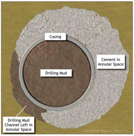
Figure 1.
Mud channel left on the narrow side of the annulus [].
Lockyear and Hibbert [] suggested that an increase in standoff had a dramatic effect on the quality of both mud displacement and cement placement. Moran and Savery [] presented a comprehensive experimental study on the effect of eccentricity and affirmed the importance of centralization. There have been indeed numerous works, such as the ones by McLean et al. [], Couturier et al. [], Jakobsen et al. [], Guillot et al. [], Chen et al. [], Foroushan et al. [], Ytrehus et al. [], Skadsem et al. [], Lund et al. [], where the importance of proper centralization and the adverse influence of eccentricity is emphasized.
In practice, there are, however, situations where the eccentricity can act in favor of the displacement process. Imagining a case of displacement in highly inclined or horizontal annuli with considerable density contrast between the displacing and displaced fluids, there are a few different possibilities that can take place. If the annulus is concentric, the denser fluid tends to gravitate more to the bottom and keep the lighter fluid on top, making a sloped interface which can become highly elongated depending on the magnitude of the density difference (Figure 2a). Having an eccentric annulus for such a case, can slow down the heavier fluid on the lower part of the annulus, resulting in a less elongated interface or ideally, if the eccentricity is set to its optimum, a nearly flat interface (Figure 2b). The other situation that can arise is that the annulus is so eccentric that the displacing fluid only flows in the larger annular sections on top (Figure 2c), which in such case the heavier displacing fluid, being on top of the lighter fluid within the elongated interface region, gravitates down to the lower parts of the annulus and replaces the mud. There is, however, a chance of contaminated cement and small channels remaining in the narrow annular gap on the bottom, as an axial displacement has not effectively taken place. According to the observations of Ytrehus et al. [], for a concentric case there could exist a sloped interface where the denser fluid flows on bottom, and when the eccentricity was increased, the heavier fluid could no longer flow axially in the narrow annulus section. This means that there is possibly an optimal eccentricity through which the heavier fluid can still flow on bottom simultaneously with the flow on top, making a flatter interface. This is in line with the work of Carrasco-Teja et al. [], in which they reported that a condition can be found where increasing the eccentricity in horizontal annuli can shorten the length of the interface. The inclination angle would, of course, influence the potential situations explained above. Therefore, there is possibly a need for more clarifications, and the research and investigations on this area can possibly be expanded.
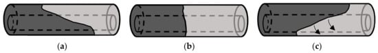
Figure 2.
Buoyancy dominant displacement in eccentric annulus, (a) negative slope front, (b) almost flat front with optimum eccentricity, (c) positive slope front with great eccentricity.
2.6. General Rules
Over the years of research, especially in the early ages, the researchers tried to develop a system of rules to follow for achieving more efficient displacements during primary cementing operations.
McLean et al. [] suggested that to prevent mud from being bypassed by the cement slurry in the narrower annular gaps, a viscosity difference is necessary. They proposed a rule, which was to have the yield strength of the cement greater than that of the mud multiplied by the largest annular gap divided by the narrowest annular gap. However, it should be noted that the cement yield stress must be still low enough for it to initiate the flow in the narrower annular sections. In line with this, Lockyear and Hillbert [] suggested that if the cement yield stress is too high, it might be impossible for the shear stress to exceed the yield stress and, thus, cement might not be able to flow into the narrow side, even if, theoretically, it is possible for mud to be displaced. Lockyear and Hibbert [] and Lockyear et al. [] proposed some generalized rules for fluid displacement. First, before the displacement, the mud gel must be broken. They suggested that the wall shear stress must be greater than the mud gel strength, as in the absence of any pipe movement, the frictional pressure drop is the only force acting on the gelled mud. This means that
where b is the width of the narrowest annular gap, is the frictional pressure drop, and is the mud gel strength.
Second, Lockyear et al. [] suggested that to keep the displaced fluid moving in the narrow annular gap, the wall shear stress generated by the frictional pressure drop of the displacing fluid, plus the difference in hydrostatic head, must exceed the displaced fluid yield stress, meaning that
where is the density, is the yield stress, and subscripts 1 and 2 denote displaced and displacing fluids, respectively. The condition of Equation (2) was also proposed by Couturier et al. []. The next requirement, according to Lockyear et al. [], was to avoid channeling by controlling the velocity of the interface in the narrow annular sections, by increasing the velocity (for example by increasing the density contrast) and/or by promoting mixing and exchange of fluids around the annulus (by running in turbulent flow regime).
According to Couturier et al. [], another desirable condition was to have the displaced fluid in the narrow annular sections running at a greater velocity than that of displacing fluid in wider annular regions. They imposed the following condition for this requirement, assuming that the displacing fluid is flowing in a channel with the size of the largest annular gap and the displaced fluid in a channel with the size of the narrowest annular gap.
Another requirement developed for horizontal (and close to horizontal) wells was suggested by Kroken et al. []. They recommended that for the displacing fluid (cement or spacer) to be able to move down the annular space to the narrow lower sections and displace the displaced fluid (spacer or mud), the buoyancy forces must exceed the inertial forces. In other words, the Froude number must be less than 1, as follows
In Equation (4), is the diameter of the wellbore and is the average velocity. For laminar displacements, Tehrani et al. [] recommended a minimum of 10 to 15% density contrast between the displacing and displaced fluids for an efficient cement placement. Moreover, Couturier et al. [] suggested that given that the flow of the displacing fluid all around the annulus is turbulent, the turbulent flow can be the most effective for the purpose of mud removal.
3. Laboratory Experimental Techniques for Fluid–Fluid Displacement
There have been numerous experimental works, such as the ones of Parker et al. [], McLean et al. [], Clark and Carter [], Martin et al. [], Haut and Crook [], Lockyear et al. [], Tehrani et al. [], Moran and Savery [], and Aranha et al. [], conducted to study the fluid displacement processes. In this section, selected experimental setups from more recent works are described to provide an overview of scales and functionality of the referred work.
The Displacement and Mixing Facility (DMF) at the University of Tulsa (Tulsa University Drilling Research Projects) was designed and built by Durmaz [] for the experiments of fluid displacement in pipes for the purpose of studying plug cementing operations. The test section was made of a transparent 2″ pipe with a length of 35 ft. Later, this facility was modified and re-built by Foroushan et al. [,,] to accommodate the experiments of fluid displacement in annuli. The outer pipe of the annulus was made of an acrylic pipe with inner diameter (ID) of 3″ and the inner pipe was aluminum with an outer diameter (OD) of 2.5″, which provided a diameter ratio of 1.2. The specifications of the test section are given in Table 1. A schematic of the experimental facility is shown in Figure 3.

Table 1.
Specifications of the experimental facility—Foroushan [].
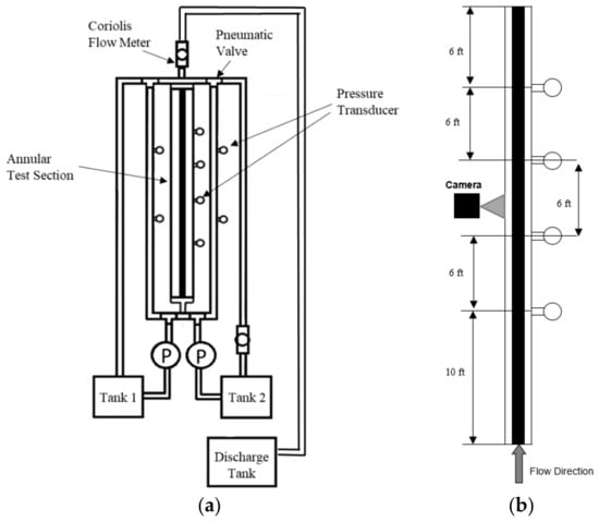
Figure 3.
Schematic of (a) experimental facility and (b) test section details—Foroushan [].
They prepared the displacing and displaced fluids in two different tanks, and to conduct a displacement test, the fluids were directed from separate re-circulation lines to the test section through the three-way pneumatic valves. Their test section could be positioned in all inclination angles, ranging from 0 degrees (vertical) to 90 degrees (horizontal). To adjust the eccentricity, Foroushan et al. [] used two in-house adjustable centralizers, which, to minimize the flow disturbance, were placed before the first pressure transducer from the inlet and right downstream the last pressure transducer. However, it should be mentioned that both test section pipes were gradually deformed with time and expecting that they could have a perfectly concentric annulus or full control on the eccentricity appeared to be too ideal. To evaluate the displacement efficiency, they recorded videos of the displacement of fluids dyed two different colors at a point 17 ft away from the inlet with a camera coverage of 2 ft. They used only one camera to record the videos, and, hence, the evaluation of the displacement was merely two-dimensional. With a length of 34 ft (10.36 m), the ratio of the length to annular gap (for a concentric annulus) was about 1632. In their experiments, the mean velocity of the flow ranged between 0.18 m/s and maximum 0.82 m/s, and the flow was always in laminar regime. They used Xanthan gum and Cesium Formate brine with water to obtain fluids with different rheological properties and densities. The rheological properties of the fluids were described by the Herschel–Bulkley model and they had fluids with density ratios ranging from 1.06 to 1.35.
An experimental setup for the displacement of fluids in an annulus was built and utilized by Ytrehus et al. [] and Lund et al. [] at SINTEF, Trondheim, Norway. Figure 4 shows the schematic of their experimental facility along with a more detailed descriptive scheme of the main components of the flow test setup. Table 2 presents the dimensional specifications of the test section. Their test section consisted of five sub-sections each with a length of approximately 2 m. The inner pipe of the annulus had an OD of 5″ and the outer pipe of the annulus, which was a transparent plastic pipe, had an ID of 6.5″ in all sub-sections, except the fourth one, where the ID of the outer pipe was 11″, representing a washout region in the wellbore. Ignoring the washout section, the ratio of the annulus length over annular gap for this setup was about 525. The inner pipe could be rotated at the rotational speed of 15 RPM. Through six fixed locations on the test section, necessary adjustments of the eccentricity and rotation could be applied to the inner pipe. Their test section could be positioned at different inclination angles, from 60 degrees inclined to 90 degrees (horizontal). To determine the displacement efficiency, Ytrehus et al. [] used both video cameras (four cameras with side view and two cameras with view from the bottom) and conductivity probes. The conductivity probes were located at four different places along the test section and at eight points (at different azimuthal angles) around the annulus. Ytrehus et al. [] and Lund et al. [] performed experiments with a mean flow velocity of 0.5 m/s and they used water-based Herschel–Bulkley fluids with density differences of approximately 10%.
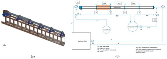
Figure 4.
Schematic of (a) test section and (b) experimental facility details—Lund et al. [].
Table 2.
Specifications of the experimental facility—Ytrehus et al. [].
The experimental facility of Ytrehus et al. [] and Lund et al. [], compared to most experimental setups previously used, appears to be quite multifunctional, as it can provide insight into both the effect of irregularities and inner-pipe rotation in highly inclined annuli.
To investigate the effect of irregularities on potential cement contamination within and above the washout sections, Skadsem et al. [] conducted full-scale experiments with water-based spacer fluids and conventional class G Portland cement slurry. Their cementing-test assembly consisted of a 32 lbm/ft 7″ tubing inside a 53.5 lbm/ft 9 5/8″ casing, with a 2.5 m long 84 lbm/ft 16″ casing as the washout section. The standoff was approximately 45% and the inclination angle was 85 degrees. The experimental setup of Skadsem et al. [] was the modified version of the one initially built and used by Aas et al. [] for the purpose of studying plug cementing and well abandonment. Aas et al. [] conducted experiments of cement placement with the tubing remained in the wellbore (9 5/8″ casing in their setup) with both conventional and expandable cements and performed pressure tests with water to investigate the sealing ability of the cement. Skadsem et al. [] measured the pressure, temperature, and fluid conductivity during the tests. Two flow rates of 18 m3/h and 48 m3/h were used for the experiments. To avoid inter-mixing of the cement with the spacer fluid inside the tubing, they were separated by a wiper ball. Skadsem et al. [] conducted leakage tests a week after the cement was placed, giving it enough time to cure. Moreover, they checked the quality of the cementing job visually, by cutting the annulus at different locations, namely, right before the washout section, in the washout section, and 2 m downstream of the washout section. Figure 5 shows their testing assembly with an example of the cut annulus after cement placement.
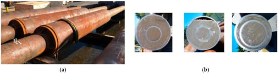
Figure 5.
Cement placement test, (a) experimental setup within washout sections and (b) cut sections after cement placement from left to right: before, in, and after the washout section—Skadsem et al. [].
More recently, Renteria and Frigaard [] presented experimental works of a dimensionally scaled lab facility for displacement of fluids in a horizontal annulus. The test section of their experimental setup consisted of four 1.2 m long transparent Plexiglass pipes with an ID of 1 3/4″ and an aluminum pipe with an OD of 1 3/8″ and had a total length of 4.8 m. Figure 6 shows the simplified schematic of their experimental facility. They used in-house eccentricity adjustment devices at five different locations of the test section to change the eccentricity of the annulus. They applied a visualization method through video cameras installed at every sub-section of the annulus to evaluate the displacement tests. To minimize the optical aberrations, each sub-section of the test section was placed inside a transparent box (fish tank in Figure 6), filled with glycerol. Renteria and Frigaard [] used a mirror arrangement, as shown in Figure 7, to reflect the bottom, back, and top views of the annulus to the cameras. They conducted experiments for fluids with the viscosity ratio in the range of 0.09 to 12, and the density difference from about 0.02% to ±16.58%.
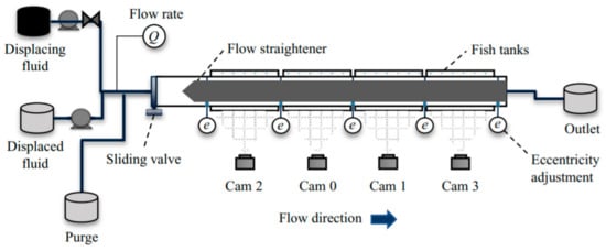
Figure 6.
Simplified schematic of experimental setup—Renteria and Frigaard [].
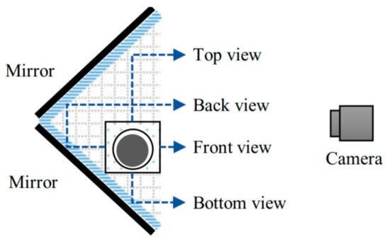
Figure 7.
Cross-sectional view of mirror arrangement—Renteria and Frigaard [].
In addition to the works discussed, it is worthwhile to mention the experimental work conducted by Ravi and Beirute [,], where an experimental device was built to investigate the mechanism involved in the erosion of the partially dehydrated-gelled (PDG) drilling mud and filter cake. The main purpose of their work was to define the erodibility of the partially dehydrated-gelled (PDG) drilling mud and filter cake and develop a procedure to improve the removal of mud and filter cake from the annulus walls in practice. Figure 8 shows a simple schematic of their experimental facility, which consisted of a pipe with an OD of 2″ inside a 5″ pipe, together placed inside a simulated formation inside a casing that was placed in a water bath. The water bath was surrounded by a temperature control medium. The total length of the test section was 18 ft, and the pressure was measured at 8 ft and 4 ft from the ends, through pressure taps that were installed on the pipes within the space between the 2″ and 5″ pipes. The space between these two pipes was sealed and the pressure taps were connected to differential pressure transducers. In order to collect the filtrate, holes were drilled on the containment casing and it could be controlled by a valve that was connected to the filtrate tank. To study the removal of dehydrated-gelled mud from the annulus during the cement placement operation, Ravi and Beirute [] proposed a 4-day experimental procedure, which was composed of: (Day 1) Calibration with turbulent flow of water and 10 min of drilling mud circulation at different flow rates with filtrate valve closed, followed by 3 h of mud circulation at three different flow rates with filtrate valve open and shut off with a differential pressure of 100 psi into the formation; (Day 2) Circulation of the drilling mud at different flow rates restarted after 18 h of shutdown, the pressure drop was monitored, and the cell was shut off with a differential pressure of 100 psi across the formation; (Days 3 and 4) The same procedure of Day 2 was followed, except that on Day 4, a spacer fluid was pumped after the mud circulation and it was then followed by cement slurry. The entire assembly was allowed to cure for 48 h and then cut to sections to visually check the quality of the cementing.
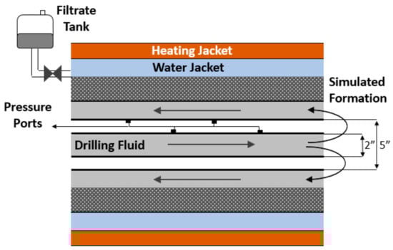
Figure 8.
Schematic of erodibility measurement experimental setup—Ravi and Beirute [].
Valuable findings and conclusions were made from the experimental results through the pressure drop measurements. Ravi and Beirute [] observed that the PDG drilling fluid and filter cake could be eroded if the pressure drop in the annulus was higher than a certain value. They proposed that if the shear stress applied at the interface of the main flow and the PDG drilling fluid layer on the annulus wall exceeds the yield stress of the PDG mud and filter cake, erosion of the mud layer and filter cake can occur. Moreover, noting that the PDG drilling mud and filter cake are packed with solid particles, they proposed a method to estimate the minimum shear stress required for the erosion of the PDG mud and filter cake to begin. To implement this method, however, one must either know the erodibility of the PDG drilling fluid or conduct similar experiments to obtain the shear stress.
Following a similar idea, Biezen et al. [] conducted experiments of drilling fluid displacement by spacer fluids, in concentric and 20% eccentric annuli to study the mud removal and erodibility mechanisms in horizontal wellbores. Figure 9 shows a schematic of their experimental setup, which consisted of an 8.5 ft annulus with a 3″-OD inner pipe and a 5″-ID outer pipe. To simulate the build-up of filter cake, they mounted a 1 ft core section on the outer pipe (shown as the hollow core section in Figure 9), through which the filtrate could be collected as the pressure was applied to the cell. The inner pipe of the annulus could be set at different standoffs and the outer pipe was exposed to a heating jacket where the temperature could be controlled and kept constant. They monitored pressure, temperature, flow rate, and electrical conductivity of the fluids during the experiments. To conduct the experiments, Biezen et al. [] followed a 3-day procedure: (Day 1) Drilling fluid circulation followed by an over-night shut-in period with no pressure applied on the cell; (Day 2) Drilling fluid circulation followed by a 24 h shut-in period with constant pressure and temperature, and hence, filter cake build-up; (Day 3) Drilling fluid removal, where a spacer fluid displaced the mud in the annulus at step-wise increasing flow rates and the removal of the drilling mud from the annulus walls could be indicated by the conductivity probes. Biezen et al. [] used real drilling fluids, which contained solid particles, that were used in North Sea operations and their spacer fluids were particularly made to possess yield stresses lower than those of the drilling muds.
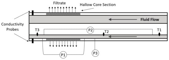
Figure 9.
Schematic of experimental setup—Biezen et al. [].
4. Displacement Flow Modelling
Although experimental works can normally provide valuable qualitative insights into fluid displacement phenomenon, they must be treated with caution when drawing generalized conclusions for establishing practical rules for field applications. The displacement flow tested in the laboratory might not successfully resemble the flow in the real field conditions, as a number of parameters can be overlooked due to the limitations caused by the nature of experimental works. For instance, as explained by Nelson and Guillot [], the ratio of casing length to the annular gap, which can be an important parameter in eccentric and buoyancy-dominant cases, has been difficult to reproduce in the laboratory in a way that the lab-scale flow dynamics would resemble those of the field. Having several of the flow dimensionless numbers matching those of the field is often attempted, but because of the complexity of the problem and number of influential parameters involved, it becomes difficult to reproduce the same field conditions in the lab. Even with all the attempts, there can always exist new displacement cases that have no similarities to the cases previously studied. Thus, a general analytical model that is able to predict the displacement efficiency and assist with finding out about possible challenges of the problem before the operation is conducted appears to be more beneficial. The physical phenomenon to be modelled is a multi-fluid flow—the displacement of one fluid by another- of non-Newtonian fluids with different properties in annuli of various eccentricities and inclination angles, running in laminar or turbulent flow regimes. Saasen et al. [] provided an evaluation of the complexities involved in experimental and theoretical studies on fluid displacement processes. When theoretical modelling is concerned, as discussed by Saasen et al. [], one of the factors that can keep the theoretical predictions different from realistic is the assumption of the no-slip condition at the annulus walls. The condition appears to be inconsistent with the cases where the annulus wall comes in contact with the displacing fluid as the interface travels forward. Moreover, Saasen et al. [] pointed out, noting that the cement and drilling fluids contain particles (solid and liquid), that the no-slip condition can only hold validity for any flow length scale greater than the largest dispersed particle. In other words, if the thickness of the mud layer on the annulus walls is comparable to the size of the solid particles in the fluids, there are high chances that other mechanisms are involved in the removal of the mud layer. The particles subjected to a shear in the region around the interface and close to the walls begin to rotate, introducing a new flow pattern in that region and contributing to the dispersion of displaced fluid into the main flow of the displacing fluid, and hence, its removal from the walls. Having a turbulent flow regime can make the situation even more complex, as the particles (both solid and dispersed liquid) can fall into interactions with turbulent eddies and, depending on eddy sizes compared to the particle sizes, different physical mechanisms can become into effect. Therefore, developing an analytical model that can address all the complexities of such a multifaceted problem does not seem trivial, and even with the recent developments in analytical and numerical computations, there still exist gaps that require more in-depth investigations.
One of the earliest attempts to include analytical calculations in the study of the fluid displacement was the work proposed by McLean et al. []. They proposed a fluid flow calculation method where they divided the eccentric annulus into sectors and treated each sector as an equivalent sector of a concentric annulus adjusted to have approximately the same gap size between the walls of the borehole and the casing. In addition to the experimental results and discussions, they provided qualitative evaluation of displacement efficiency based on the calculated ratio of the mud velocity to the average velocity of cement in the annular space. Later, Flumerfelt [] developed an analytical model for displacement of non-Newtonian power-law (PL) fluids in parallel plate and narrow-gap concentric annuli. The work was followed by the one of Beirute [] where mathematical models to describe the displacement of non-Newtonian PL fluids, under laminar flow conditions in a vertical pipe and parallel plates (narrow-gap concentric annuli), were developed. Beirute and Flumerfelt [] also proposed a displacement flow model with a similar approach for a more general rheological model, Robertson–Stiff. They determined the interface axial position through temporal integration of the velocity of fluid particles at the interface. As stated by themselves, the models were offering an approximation and one of the major problems was that there was discrepancy between the displaced volume calculated, based on the location of interface, and the actual volume of fluid flowing into the calculation domain. Hence, there were cases that their model would show a mass balance inconsistency. These were mostly the cases where the physical properties of the displacing and displaced fluids were significantly different, and the problem would start fading as the properties of the fluids approached each other. Thus, their model was not able to provide accurate quantitative predictions for severe cases of unstable interfaces that were axially elongated. Flumerfelt [] and Beirute [], however, tried to resolve this problem by introducing a correction factor to the calculation of displaced volume. They concluded that increasing the density, viscosity, and yield stress ratios and decreasing the displacement flow rate increases the breakthrough time, hence, providing better displacements.
Bittleston et al. [] and Pelipenko and Frigaard [,] proposed 2-D numerical models based on the Hele–Shaw approach for the laminar displacement of visco-plastic fluids in eccentric annuli, where they used a classical dimensional scaling method to reduce the three-dimensional equations of motion to a two-dimensional gap-averaged model. They mapped the narrow eccentric annulus geometry to a Hele–Shaw cell geometry, as shown in Figure 10, and derived the flow equations in the new transformed system of coordinates.
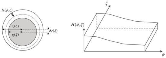
Figure 10.
Narrow eccentric annulus mapped to Hele-Shaw cell—Pelipenko and Frigaard [].
Bittleston et al. [] derived a coupled system of equations that consisted of a quasi-linear Poisson-type equation for the stream function of bulk fluid flow, a series of first-order convection equations for the fluid concentrations, and closure expressions for the fluid properties in terms of the gap-averaged fluid concentrations. Their final model can be summarized as the following equations.
with constitutive relations:
the stream function definition
and the concentration equations
Equations (6) and (7) are obtained from the constitutive laws of visco-plastic fluids and imposed the condition that a Herschel–Bulkley fluid needs to start flowing (meaning that the fluid does not move if subjected to a shear stress less than its yield stress). In Equations (5)–(9), and are the azimuthal divergence and gradient operators, respectively, contains the buoyancy term, is the local mean radius of the annulus, is the stream function, is a positive increasing function of , arising from the viscous shear-thinning behavior of the fluids, is the annular gap half-width, is the fluid yield stress, and are the gap-averaged velocities, and is the gap-averaged concentration of fluid . Bittleston et al. [] used the flux-corrected-transport (FCT) scheme to explicitly solve the concentration at each time step and a hybrid asymptotic-numerical method to solve Equation (5). For any given flow rate, the stream function could be obtained through Equations (5)–(7). This would make it possible to obtain the velocity fields via Equation (8), and advance the fluids concentration in time by Equation (9). The authors assumed that the fluids were homogeneous across the annular gap and ignored the dynamics of the flow in the vicinity of the interface by scaling laws. One of the assumptions that could highly contribute to numerical dispersion was the use of closure expressions for rheological properties of the fluids, such that the Herschel–Bulkley parameters followed the mixture laws, meaning that, for example, the flow index n could be defined as .
As a whole, the model developed by Bittleston et al. [] offered an advancement in modelling of the fluid displacement in eccentric annuli and predicting the quality of the fluid displacements, and appeared successful in alerting the user about potential failures in the cementing job. One of the most challenging cases studied within their work was the displacement of drilling mud (density = 1440 Kg/m3, flow behavior index = 0.7, consistency index = 0.02 Pa-s, and yield stress = 4.79 Pa) by spacer (density = 1440 Kg/m3, flow behavior index = 1, consistency index = 0.01 Pa-s, and yield stress = 3.76 Pa) through an 11-inch washout section from 800 m to 900 m depth, and a 50%-eccentric section from 1200 m to 1300 m depth. The casing is 8 ½ inch with a hole size of 9 5/8 inch. The eccentricity of the rest of the annulus was 20%, and the spacer was followed by a cement slurry (density = 1800 Kg/m3, flow behavior index = 1, consistency index = 0.03 Pa-s, and yield stress = 7.05 Pa). Looking at the predictions provided in Figure 11, the spacer appeared to be inefficient in displacing the drilling mud, especially within the two mentioned challenging intervals, where it bypasses the mud in the narrower annular sections. Cement seemed to efficiently displace the spacer, which could be expected for the cement having a considerably higher density and viscosity. However, considering the model assumptions earlier discussed, doubts and questions can be raised about the accuracy of the inter-fluid mixing and cement contamination, as the model is derived based on a gap-averaging approach and cannot predict the existence of the mud layer left on the casing and wellbore walls due to elongated interfaces in the annular space at every azimuthal angle. The authors argued that although the case studied seemed to present numerical diffusion, the important message is delivered to the user: the cementing job might involve mud channels on the narrow sides and cement contamination.
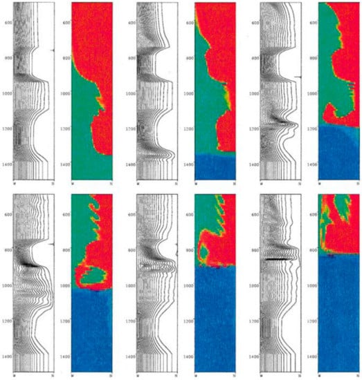
Figure 11.
Cement–spacer–mud displacement-flow streamlines and fluid concentration at times = 600, 800, 1000, 1200, 1400, and 1600 s (from left to right, top to bottom)—Bittleston et al. [].
Moreover, the case studies presented in the paper did not include stand-off values lower than 50%, which can generate a question if the model is able to accurately predict the existence of a mud channel within the narrow annular sections in more severe cases of eccentricity.
Following the work of Bittleston et al. [], Pelipenko and Frigaard [,,] extended their model to the case where there was a distinct interface between the displacing and displaced fluids. In that way, the entire flow domain was divided to two sub-domains of displacing and displaced fluids, and the equation of concentration was replaced by an interface tracking formulation which included the gap-averaged kinematic description of fluid interface along with normal and tangential boundary conditions at the interface. Pelipenko and Frigaard [,] investigated the uniqueness of the solution of Equation (5) for either of the concentration-based or interface tracking-based methods within the practical range of conditions. They concluded that the model by Bittleston et al. [] is mathematically sensible and that for reasonable distributions of fluid concentrations or interfaces, there existed a unique solution to stream function. Moreover, they explored the possibility of the occurrence of steady state displacement flows, in which the interface seems to travel steadily, and they provided analytical solutions to stream function and interface shape for steady-state displacements in concentric and slightly eccentric annuli. They studied the effect of different rheological parameters on the shape of the interface and the solutions and results suggested that steady-state displacements can take place during the cementing operation. The work, however, could not provide insights into the instability of the displacement flow. In another work, Pelipenko and Frigaard [] offered a numerical solution to the model of Bittleston et al. [] and alternatively to the one based on interface tracking formulation (Pelipenko and Frigaard [,]) for sections of wellbores with constant geometrical specifications. Compared to three-dimensional computational approaches, their model was aimed to provide a more convenient solution method in terms of numerical complications and computational time, as it was developed for a two-dimensional gap-averaged Hele–Shaw cell where various scaling arguments were used to reduce the three-dimensional Navier–Stokes equations to a two-dimensional system only in axial and azimuthal directions. Pelipenko and Frigaard [] presented a discussion on the instability of the displacement front and divided the cases to three possible categories: (i) stable steady-state interfaces (such as a travelling wave (Figure 12a), (ii) stable, but unsteady mobile interfaces (both fully mobile fluids (Figure 12b) and burrowing motions (Figure 12c), and (iii) stable unsteady interfaces that are immobile on the narrow side of the annulus (Figure 12d).
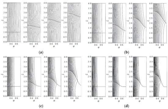
Figure 12.
Stream function and interface progress: (a) steady state, (b) unsteady mobile interface, (c) unsteady burrowing, (d) unsteady immobile—Pelipenko and Frigaard [].
The instability discussed by Pelipenko and Frigaard [] is not a local interface instability but is a global displacement flow instability. The authors argued that since the displacements of cementing operations are always designed in a sensible way that the heavier and more viscous fluid displaces the lighter and less viscous fluid, the interface always stays stable, and thus, only the steady/unsteady motion of the interface and its general pattern within the displacement flow is of concern. There are a few important points, however, that must be noted. A proper design of fluids for an efficient cement placement is not a trivial task and the industry, knowing that density and viscosity hierarchies must be held, still happens to have to deal with inefficient displacements. Therefore, an interface instability analysis can become considerably beneficial in determining the onset of the instability, and thus, the most suitable fluid properties and flow rate for an optimized displacement. Moreover, in the cases that the interface is elongated due to eccentricity and/or high inclination angle, there will be regions with parallel motion of the displacing and displaced fluids. Fluids with different properties running at different velocities at each side of the interface in such regions can generate a Kelvin–Helmholtz type of instability. Studying the instability of the interface in such regions can assist with finding out if the instability is in the favor of the displacement, as it can promote a motion of the slower or nearly static fluid on the other side, or it causes inter-fluid mixing and results in more cement contamination without contributing much to the displacement process.
Having a model that obtains the flow field in the annular gap can be not only useful, but also essential for a lot of cases, because even with apparently reasonable density and viscosity hierarchies, having a flat interface in the annular gap is unlikely and different properties of the fluids result in different (local) interface shapes in the annular gap. Figure 13a,b, as examples to this discussion, present the effect of PL rheological properties of fluids on the shape of the interface between two vertical plates, studied by Flumerfelt []. According to this study, increasing the consistency index of the displacing fluid, while keeping all other properties the same as those of the displaced fluid, can provide a flatter interface, whereas decreasing the flow behavior index of the displaced fluid can result in a more elongated interface.
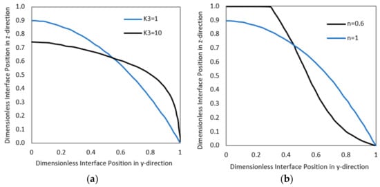
Figure 13.
Effect of fluid rheology on the interface shape: (a) effect of consistency index, (b) effect of flow behavior index—Flumerfelt [].
Similar discussions on the interface shape were presented by Taghavi et al. [], where they developed a model for buoyancy-dominant displacement flows in near-horizontal channels, where the heavier fluid tends to flow on the bottom of the channel, keeping the lighter fluid on top. Figure 14a shows the effect of viscosity for Newtonian fluids, whereas Figure 14b presents the effect of the flow behavior index for non-Newtonian fluids. In both figures, the density of the displacing fluid is greater than that of the displaced fluid. Figure 14a shows the calculated interface shape for three different viscosity ratios of Newtonian fluids, where m is the ratio of the viscosity of the displaced fluid over the one of the displacing fluid. Decreasing the ratio helps to have a less elongated interface, as expected. The results of Figure 14b, however, could not easily be guessed. The case of a low generalized viscosity ratio (m = 0.1), with flow behavior indices of 0.25 and 1 for displacing and displaced fluids, respectively, is compared to a case with a greater generalized viscosity ratio (m = 10), with flow behavior indices of 1 and 0.25 for displacing and displaced fluids, respectively. It appears that the first design provides a shorter and flatter interface, hence potentially better displacement. This is a conclusion that could not be easily drawn on the field, without proper model calculations and, thus, a confirmation that the design of the displacement fluids is not as simple as it may sound by the rule of thumb of “keeping density and viscosity hierarchies”.
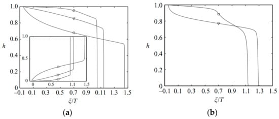
Figure 14.
Effect of fluid rheology on the interface shape: (a) viscosity ratio: m = 0.1 (o), m = 1 (∆), m = 10 (□), (b) generalized m = 0.1, nH = 0.25, nL = 1 (∆), m = 10, nH = 1, nL = 0.25 (□)—Taghavi et al. [].
An elongated (local) interface region is expected to leave thicker mud layers on the wellbore and casing walls, resulting in contaminated and incomplete cementing job. Although two-dimensional gap-averaged models, such as the one of Bittleston et al. [] and Pelipenko and Frigaard [,,,], can give qualitative insights into the potential of such problems, they cannot provide quantitative predictions of the mud removal between the wellbore and casing walls and closer to the walls.
Szabo and Hassager [] used the arbitrary Lagrange–Euler (ALE) finite element technique to simulate 3-D displacements of Newtonian fluids in vertical eccentric annuli. They also proposed a simple expression for the displacement efficiency based on an idealized lubrication theory and suggested that the ratio of the displacement length to the gap width, provided that it is sufficiently large, does not affect the displacement efficiency. This was supported by their simulations as well. However, the simulations were performed for a limited combination of dimensionless numbers and eccentricities, and more simulations were probably needed to establish a firm conclusion in this regard. Rasmussen et al. [] proposed an improvement to the work of Szabo and Haasager [], where they used the Lagrange–Euler finite element method with a streamline upwind Petrov–Galerkin formulation for the computations of the interface condition. This gave them the chance to simulate the displacement in longer annuli at different inclination angles, differently from the work of Szabo and Haasager [] where the total amount of the fluid pumped corresponded to a displacement length less than 9 times of the annular width and only vertical displacements were considered. Moreover, Rasmussen et al. [] concluded that the lubrication theory could not predict the shape of the displacement front and was only valid for vertical wells.
Savery et al. [] developed a numerical 3-D simulator to model the fluid displacement and mixing in eccentric annuli with irregularities and washout sections. For computational convenience in dealing with an irregular-shaped outer boundary, they applied a boundary-conforming curvilinear coordinate transformation, and to calculate the displacement and inter-mixing, they used a convection-diffusion equation for fluid concentration. The numerical model could also handle the case of casing reciprocation and rotation, where they showed that rotating the casing could act in the favor of displacement. Perhaps an important piece of information that was missing in the work of Savery et al. [] was about the computational time and cost to simulate the displacement process in a realistically long portion of a wellbore.
A new generation 3-D simulator was more recently introduced by Tardy et al. [], where a high-resolution annular displacement model, accounting for the complex 3-D annulus shape with full determination of axial and azimuthal flows was developed. Tardy [] provided theoretical details of the model where the lubrication theory with narrow-gap approximation was used to solve the 3-D velocity and concentration fields along with a 2-D elliptic pressure equation. A finite volume method was used to solve the equations numerically, and this required a lower CPU time than fully 3-D Computational Fluid Dynamics (CFD) computations, although possibly still greater than the simplified 2-D models. Moreover, their model was well validated against experimental works of Ytrehus et al. [] and CFD simulations by ANSYS FLUENT.
The fully 3-D models, being capable of capturing the details of the flow dynamics, are expected to provide the most accurate and realistic predictions on the quality of the fluid displacement process and a better understanding of its complications. However, they are often found to have limited practical applications because of their complexity, and the fact that numerical methods and CFD, although providing powerful tools for more accurate calculations, require a great deal of knowledge and expertise to present their best computational performance. Therefore, a model, such as the one of Tardy [], that is kept computationally simple, but also with an attempt to exclude some of the theoretical simplifications of the previously developed models, becomes considerably useful practically.
Following the idea of flow in a narrow slot, Foroushan et al. [,,] proposed a model for displacement of fluids in narrow eccentric annuli at different inclination angles. Through the conservation of momentum, they solved a Poisson-type of differential equation with an irregular boundary, because of the unwrapped annulus, for each fluid region. They assumed symmetry along the x-axis and solved only for half of the unwrapped annulus, shown in Figure 15. To solve for the displacement flow, they used the flow solution in concentric annuli at the largest and narrowest gaps of the annulus as the boundary conditions. This meant that the change of the shear stress in the z-direction was negligible only at these two locations, which with the assumption of symmetry was a legitimate approximation.
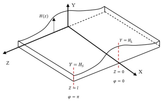
Figure 15.
Unwrapped eccentric annulus configuration—Foroushan et al. [].
To solve for the shape and location of the interface, they used the condition of kinematics of the interface. Noting that depending on the inclination angle, the interface could form itself into different shapes as previously pointed out by Taghavi et al. [] and Rasmussen et al. [], Foroushan [] proposed displacement solutions for three categories, each of which would present similar shapes of the interface. These were: (i) displacement in vertical or nearly vertical wells with symmetric interface, including the cases of other inclination angles with insignificant density contrast, (ii) displacement in horizontal or nearly horizontal wells with dominant buoyancy effects, when the heavier fluid has the tendency to stay on the bottom, and (iii) displacement in inclined wells. The main model equations for displacement in vertical annuli were given as below. The momentum equation at each fluid region
was solved with the following boundary conditions for each fluid zone:
Fluid 1 (displaced fluid)
and Fluid 2 (displacing fluid)
coupled with kinematics of the interface as follows.
In Equations (11) and (12), and are the solutions of the velocity field of Fluid i at the largest and narrowest annular gaps, respectively, corresponding to flow solutions in concentric annuli with annular gaps HL and HS, respectively. In Equation (13), is the distance between the interface and the adjacent wall within Fluid 1 (displaced fluid) region, and is the flux of the displaced fluid. They obtained the solution of the flow analytically and used it to find the interface solution numerically through Equation (13). This offered a solution method with a considerably lower computational time compared to the fully numerical and CFD models. Foroushan et al. [] used the concept of apparent viscosity and calculated a variable apparent viscosity along the annular space, as the shear stress and shear rate are expected to change with the annular gap size. They tested the method for power-law (PL) and yield-power-law (YPL) fluids and validated the results against CFD simulations of ANSYS FLUENT. The model of Foroushan et al. [,] was used to simulate a few of the experimental cases of Lund et al. []. The displacements under study include the experiments E, G, I, and J in the work of Lund et al. [], which are displacements in 42% eccentric annuli at horizontal (Exp G and Exp I) and 60 degrees inclined (Exp E and Exp J) configurations, with a flow rate of 15.7 m3/h (mean velocity = 0.5 m/s). In all the cases, the displaced and displacing fluids have densities of 1000 and 1100 Kg/m3, respectively, and the rheological properties are given in Table 3, reported based on the dimensionally consistent formulation of Saasen and Ytrehus [], also explained in []. Figure 16 and Figure 17 illustrated the displacement efficiency calculated based on the model of Foroushan et al. [] compared with experiments run at SINTEF provided in the work of Lund et al. []. In general, the displacements appear to be improved as the inclination angle decreases according to both experiments and analytical model. The analytical model, however, does not predict as great of a difference in the displacement efficiency as the experiments, as the inclination angle decreases. For the displacement cases I and J, the breakthrough, according to the model, at both inclination angles appears to happen earlier than that of the experiments. This can be because the analytical model uses the concept of apparent viscosity and the calculated variable viscosity at certain annular gaps (especially the narrower section) might not be accurately representing the rheology of the fluids. On the other hand, noting that the increase in the displacement efficiency with a change of the annulus configuration, from horizontal to 60 degrees inclined, is only attributed to the density difference, which is the same in both groups of experiments; having the increase in efficiency in group E and G be not as significant as in group I and J suggests that the rheological properties of the fluids used in the experiments were not exactly the same as each other and as the ones used in the model. Moreover, the experimental results correspond to displacement cases with a washout section, which was not considered in the analytical model simulations.
Table 3.
Properties of displacement fluids—Lund et al. [].
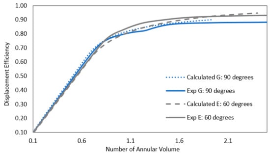
Figure 16.
Comparison of displacement efficiency for cases E and G—experiments by Lund et al. [] and model by Foroushan et al. [].
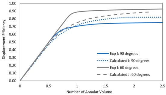
Figure 17.
Comparison of displacement efficiency for cases I and J—experiments by Lund et al. [] and model by Foroushan et al. [].
5. Fluids Interface
The instability of the displacement flow can be perhaps viewed from two perspectives: the local view of interface instability and the global view of the entire front and its progress with time. This means that in an annulus, the interface can be looked at locally, moving between the walls in the annular gap, and globally in a larger scale as the whole displacing fluid front progresses. Although the dynamics of these two are not independent, having a locally stable interface does not necessarily guarantee that the displacement front will not be elongated and possibly discontinued at places along the way. This is because other factors such as eccentricity, geometric irregularities, and inclination angle can greatly affect the shape of the global interface. A suitable terminology for the way the interface evolves globally is perhaps to define it as stable steady or stable unsteady, as was suggested by Pelipenko and Frigaard [], instead of stable or unstable. Generally speaking, the shape of the interface can define how effective the displacement can be. Elongated and unstable are normally associated with channeling, resulting in excessive inter-fluid mixing and cement contamination. Interfacial instability in a fluid system can be characterized by material interpenetration, which implies the effects of density and viscosity, and mixing at molecular scales, which implies the effect of surface tension or lack thereof. Among the hydrodynamic instabilities, the two that can be most related to the case of fluid displacement are Rayleigh–Taylor and Kelvin–Helmholtz instabilities, understanding of which can be an important starting point in comprehending the interfacial interactions and displacement flow dynamics during mud removal and cement placement processes.
5.1. Rayleigh–Taylor Type of Instability
Rayleigh–Taylor instability is a buoyancy-driven instability and occurs in superposed fluid flow systems that contain fluids with different densities in the presence of acceleration, such as gravity. The instability of the interface between two superposed Newtonian fluids was initially studied by Rayleigh []. In that study, he assumed that the fluids had different densities and that they were initially at rest with the denser fluid on top of the lighter one.
Later, Taylor [] included the effect of a constant acceleration acting perpendicularly to the interface. He pointed out that when two superposed fluids of different densities and negligible viscosities are accelerated in a direction perpendicular to their interface, this surface could be stable for small deviations if the acceleration is directed from the denser to the less dense fluid.
The original Rayleigh–Taylor instability assumes that the fluids are inviscid, and the superposed fluids are stationary before any disturbance occurs at the interface. It states when the heavy fluid sits on top of the light fluid, any small perturbation at the interface grows exponentially with the temporal growth rate of:
where A is the Atwood number, defined by
g is gravitational acceleration, and are the density of the fluid on top and bottom, respectively, and k is the spatial wave number. It can be seen that for negative Atwood numbers, when the density of the top fluid is less than another, the interface will stay stable, whereas a positive Atwood number guarantees that the growth rate is a positive real number, resulting in the exponential growth of the interfacial disturbance with time.
A more general model that includes both viscosity and surface tension of the fluids has been developed by Chandrasekhar []. The research in this area has benefited from the vast contribution made by Mikaelian [,,]. Mikaelian [] studied the turbulent mixing generated by Rayleigh–Taylor instability and provided discussions on the size of the eddies generated by this instability. The two main conclusions were that the largest eddy size and the mixing length are related (the largest eddy generated is 40% of the mixing length), and the large eddies were at least ten times larger than smallest eddies. Mikaelian [] studied the effect of the viscosity on the turbulent energy generated by the Rayleigh–Taylor instability, and concluded that the viscosity had a damping effect.
Foroushan et al. [] made use of the analyses performed by Chandrasekhar [] and Mikaelian [], and based on a perturbation approach developed an instability model for a Rayleigh–Taylor type of instability, where the steady velocity solution of the fluids under the base unperturbed condition was taken into account. In this way, they could investigate the effect of the flow rate as well as other physical parameters. They applied the moment technique proposed by Mikaelian [] to the general 4th-order perturbation equation obtained as
and found an expression for the temporal growth rate of the perturbations as follows.
where is the general acceleration term in z-direction, which is related to the pressure drop and densities of both fluids in the domain, A is the Atwood number, is the ratio of sum of viscosities to sum of densities, and are the densities of displaced and displacing fluids, respectively, and and are the viscosities of displaced and displacing fluids, respectively. Through this analysis, Foroushan et al. [] showed that, finding the onset of instability for different design parameters, improvements on the design of the displacement process could be suggested in order to keep the interface as stable as possible. In a case study, they showed that for a displaced fluid with density = 1546 Kg/m3, flow behavior index = 0.785, consistency index = 0.209 Pa-s, and flow rate = 50 gpm, in an annulus with the size of 3 inch × 2.5 inch, the density ratio must be at least 1.28 if the displacing fluid has the same viscosity, and the ratio of the apparent viscosity in a concentric annulus must be at least 1.26, if the densities are the same (see Figure 18).
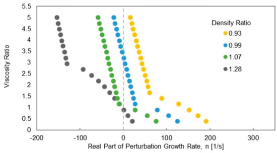
Figure 18.
Effect of density and viscosity of fluids—Foroushan et al. [].
According to the discussions by Foroushan et al. [], increasing the flow rate increases the chance of interface instability. They suggested that there exists a maximum flow rate above which the interface becomes unstable. Figure 19 shows an example of such a study for a displaced fluid with density = 1546 Kg/m3, flow behavior index = 1, consistency index = 0.0312 Pa-s, and yield stress = 9.7 lbf/100 ft 2, and displacing fluid with density = 1618 Kg/m3, flow behavior index = 0.428, consistency index = 1.889 Pa-s, and yield stress = 5.88 lbf/100 ft 2. They concluded that in this case, for the flow rates above 38 gpm (0.904 bpm) the interface becomes unstable and some mixing can be generated.
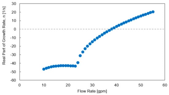
Figure 19.
Effect of displacement flow rate—Foroushan [].
Moreover, it was shown by Foroushan [] that keeping the average annular velocity unchanged, depending on the properties of the displacing and displaced fluids, changing the annular size can make the interface stable/unstable. For a displacement case, with the displaced fluid (density = 1546 Kg/m3, flow behavior index = 0.787, consistency index = 0.189 Pa-s, yield stress = 1.87 Pa) and displacing fluid (density = 1582 Kg/m3, flow behavior index = 0.295, consistency index = 4.088, yield stress = 0), it was observed that the interface could stay stable in a wellbore-casing size of 12 ¼″–9 5/8″, while unstable in a borehole-casing of 8 1/2″–7″and a lab-scale annulus of 3″–2.5″. Figure 20 shows that, for this combination of fluids, as the borehole size and diameter ratio increase, the interface becomes more stable. A borehole size of 8 1/2″ requires a diameter ratio greater than 1.37 for the interface to stay stable, whereas a borehole size of 12 ¼″ with a diameter ratio of 1.27 can be stable.
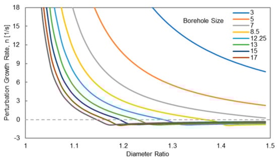
Figure 20.
Effect of annulus size—Foroushan [].
It should be noted that the instability study by Foroushan et al. [] is based on a method where the growth (or decay) rate is only temporal, meaning that the wavenumber is a real number, which is different from the case that the spatial growth (or decay) of the interfacial disturbance is studied with a complex wavenumber as a function of disturbance frequency.
Concerning Rayleigh–Taylor instability for non-Newtonian fluids, the works carried out by Saasen and Tyvand [], Saasen and Hassager [], and Sharma and Sharma [] can be mentioned, where the instability of superposed viscoelastic fluids was studied. It was shown that the interface can become more unstable as the length of the disturbance increases. This means that in the cases with potentially longer interfaces, such as in inclined annuli, more instabilities can be observed than in a case similar to vertical annuli. Sharma and Sharma [] studied Rayleigh–Taylor instability of particle-laden superposed fluids and concluded that the presence of particles did not change the results of the instability.
Focusing on a case where the global fluid interface is elongated due to the eccentricity, it can happen, especially if the wellbore is inclined, that the heavier fluid is superposed on top of the lighter fluid, and the Rayleigh–Taylor instability coming into act, the denser displacing fluid moves down and replaces patches of the displaced fluid, pushing them to the higher-velocity flow regions. This was observed by Tehrani et al. [], where they suggested that gravity-driven azimuthal instabilities can help the displacement in the narrow annular side, although patches of the mud might be left trapped at regions. Similar discussions and observations were carried out by Jakobsen et al. [], Szabo and Hassager [], and Ytrehus et al. [].
5.2. Kelvin–Helmholtz Type of Instability
The Kelvin–Helmholtz instability was first described by Helmholtz [], but the problem of instability was first posed and solved by Kelvin []. The original model was developed for two stratified fluids, with horizontal velocities, and a relatively horizontal interface separating the two fluids and with a velocity difference or gradient across the interface. In this case, the region on the upper fluid that is carried down for the perturbation will be dragged horizontally with the lower fluid. This results in vorticity generation at the mixing layer and the interface will roll up with the direction of the vorticities. If the viscous dissipation is high enough to dissipate the vorticity’s energy, the interface will stay stable.
During the cementing operations, the interface between the two fluids can become elongated, either because of improper design of the fluids, or because of eccentricity and/or high inclination angles. In such a case, a part of the flow along the elongated interface can be represented by stratified flow, where the fluids move in the same relative direction as the interface position. Under this condition, depending on the properties of the fluids and relative velocities of each fluid region, the interface can experience a Kelvin–Helmholtz type of instability.
From a mud-removal point of view, a stable Kelvin–Helmholtz interface might result in an incomplete cementing, leaving a thin mud film on the annulus walls. Thus, initiation of an unstable interface that develops vorticity-like motions in the stratified flow section closer to the walls can be perhaps a favorable phenomenon. Figure 21 displays CFD simulation results of Foroushan et al. [] for the case with a mud layer left on the annular wall (on top) and a case where the Kelvin–Helmholtz instability disturbs the mud layer and contributes into its removal.
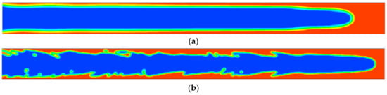
Figure 21.
Instability of interface in fluid displacement, (a) stable K–H (0.5 s), (b) unstable K–H (0.5 s)—Foroushan [].
The problem of the Kelvin–Helmholtz instability for fluids with different densities and viscosities has been analytically studied by Chandrasekhar [] and Drazin and Reid [] through a perturbation method. Within these studies, the base unperturbed case is normally considered as a laminar steady-state flow solution, similar to the one earlier explained for Rayleigh–Taylor instability. There have been works, such as the ones of Kuru et al. [] and Cohen and Hanratty [], where one of the phases was running in turbulent. Kuru et al. [], who performed a linear instability analysis of the stratified channel flows, concluded that, first, only small differences were found in the growth rate of disturbances between laminar and turbulent flows of air over water, if the friction velocity and the liquid height were the same. Second, they suggested that the primary effect of turbulence was found to be through changes in the time-averaged velocity profile. This was supported by Cohen and Hanratty [], where they observed that the liquid film can hold a smooth interface even if the flow of the other phase is turbulent, as long as its flow rate is below a critical value. These observations, however, were only for air–liquid systems, and their validity for liquid–liquid needs to be investigated. Frigaard [] performed a linear instability analysis for parallel flows of Bingham Plastic fluids for which an unyielded plug region was adjacent to the interface. The main conclusion of this work was that a long unyielded fluid region would not suffer from the classical linear interfacial instabilities produced by an infinitesimal perturbation. Sahu et al. [] analyzed the linear instability of a Newtonian fluid on a non-Newtonian YPL fluid, where the non-Newtonian fluid layer was yielded, because of high pressure drops. They used the linear perturbation method to derive an Orr–Sommerfeld eigenvalue problem for low wavenumbers and concluded that increasing the values related to the yield stress and flow behavior index can induce instabilities, especially when the thickness of the non-Newtonian layer is large.
During the mud displacement/cement placement, normally to avoid problems due to incompatibility of cement slurry with drilling mud, a preflush fluid is pumped between the mud and cement. The preflush fluid, in addition to being compatible with both the drilling mud and the cement, is expected to possess desirable physical and chemical properties to enhance the mud removal and help to achieve a complete cement placement with minimal contaminations. The preflush fluids can be divided in two categories: (i) a wash fluid, which normally has a low density and viscosity (such as water) and can run in turbulent, and (ii) a spacer fluid, which ideally has an optimal design of density and rheological properties to ensure an effective mud removal. The fluids are expected to have proper chemical properties to make sure that the annular surfaces are left clean and water-wet for the cement slurry to create a strong bonding. A cementing job can include one, both these fluids, or a chain of washes and spacers between the drilling mud and cement slurry. As discussed, one of the problems that can become troublesome and lead to issues such as inter-zonal communication and annular fluid migration, and possibly environmental hazards, is the inefficient removal of the mud layer on the walls of the wellbore and the casing. Therefore, more research on the instability of the interface in this region and dynamics of the flow for the mud layer removal, under laminar and turbulent flow regimes, is beneficial and perhaps necessary. From the mechanical point of view, the main idea to remove the mud layer after displacing the bulk drilling mud is to agitate the surface of the mud layer left on the walls so that lumps and particles of the drilling mud can become detached from the wall and be carried out with the main flow. Thus, creating an unstable interface can help this process, and both of the instability types discussed above would come to action. As explained, Rayleigh–Taylor instability can induce turbulence locally, generating eddies around its mixing length. To provide a visual idea, the work of Rahman and San [] can be mentioned, where they performed high-resolution numerical simulations for both multi-mode and single-mode inviscid Rayleigh–Taylor instability. Figure 22, from their work, shows the time-evolution of density field (or interface between the two fluids) for a single-mode Rayleigh–Taylor instability. The signs of chaotic mixing and induced Kelvin–Helmholtz instability can be seen within the mixing length. This means that, although a stable interface is desired for the stage of the cement placement, an unstable interface as such can help generating disturbances and eddies around the interface and even lead to a secondary instability, namely, Kelvin–Helmholtz.
Figure 22.
Time evolution of Rayleigh–Taylor instability: (a) t = 1.8, (b) t = 2.7, (c) t = 3.6, (d) t = 4.5—Rahman and San [].
In addition to having the right properties of the fluids for generating this instability, a flow rate above the critical one can help to induce more disturbances at the interface region, promoting Kelvin–Helmholtz instability. Moreover, a turbulent flow regime, because of its chaotic and stochastic nature, appears to help the process of mud entrainment into the main flow. Running the primary displacement flow in turbulent for cement placement has not been proven to provide better displacements. As earlier discussed, some works such as the ones of Foroushan et al. [,] and Yerubandi et al. [] suggested that keeping the flow rate below a certain level provided better displacements. McLean et al. [] concluded that the turbulent flow did not offer a better displacement, and thinning the cement to run it in turbulent regime caused additional channeling. More recently, Maleki and Frigaard [] compared the performance of laminar and turbulent flows of spacer fluids displacing a drilling mud, and stated that no firm and clear conclusion could be drawn that the turbulent flow resulted in more efficient displacements, as there were cases where the laminar flows performed better. They also suggested that the performance of the preflush fluids should be judged based on the frictional pressure drop that they generate, regardless of the flow regime. This was previously discussed by Nelson and Guillot [], where they stated that having a turbulent flow alone is not sufficient and unless the fluid running in turbulent has a frictional pressure drop at the same level as the one of a viscous fluid displaced under laminar conditions, the displacement would not be efficient. However, as mentioned by Nelson and Guillot [], because of the complicated mechanisms involved in turbulent flow displacement, finding the conditions for efficient turbulent flow is more difficult. Guillot et al. [] studied the effectiveness of preflushes on the displacement efficiency through numerical simulations, and concluded that although washes appeared to have a tendency to run in the wider annular part and in some cases do not prevent the direct contact between the fluids, in general, they can be effective when instabilities are induced, promoting mixing and dispersion of the drilling mud into the wash. Although the combination of turbulence, Rayleigh–Taylor, and Kelvin–Helmholtz instabilities seems to provide a condition for agitation and dispersion of the mud layer into the flow of the preflush fluid, an in-depth investigation of the phenomenon for nonlinear deformations of the interface with non-Newtonian fluids and affected by turbulence can definitely assist with the establishment of guidelines for more efficient mud removal and eventually cementing jobs. Biezen et al. [] conducted experiments of drilling fluid removal in horizontal annuli with lower-yield stress spacer fluids mixed with surfactants and observed that, in a concentric annulus, the top section was cleaned at a mean velocity of 0.205 m/s (laminar flow), whereas the bottom side of the annulus required a mean velocity as high as 1.13 m/s (turbulent flow) to be cleared and water-wetted. They recognized the problem as the drilling fluid being so light (specific gravity of 1.25) that it displayed low abilities in keeping the barite suspended during the static periods. Therefore, high flow rates were needed to disperse and remove the fluid packed with settled barite from the lower annular section. Furthermore, as previously discussed, the dynamics of the flow and fluid interaction can be altered, knowing that the fluids contain particles subjected to rotational motions in the vicinity of the interface and within the displaced fluid layer on the walls. In addition, depending on the size of the particles, the way they may interact with each other and be packed in the film region, and the shear history within the mud layer on the wall, the properties of the fluids can be different closer to the walls. Altogether, these might suggest that a closer look into the vorticity of flow and different methods of instability analysis might be necessary in future.
6. Conclusions
The present overview contains a brief review of theoretical, experimental, and field studies conducted over the years to assist the industry with overcoming the challenges that it faces during primary cementing operations. Although there have been general rules developed to be used in practice during fluid displacement processes, it appears that the methods could yet be improved as there are still unresolved challenges that can lead to inefficient displacement and cement contamination. The current review covers an overall idea on the progress made in the field of fluid displacement, and thereby identifies the technology gaps that can be addressed to assist enhancing the cement placement jobs.
Although it is known by the industry that, for an efficient displacement, the displacing fluid must have higher viscosity and density than the displaced fluid, the theoretical work could still be improved to provide insight into potential challenges of a work for an optimized design of fluids prior to the cementing job. Moreover, there might exist cases where the density and viscosity hierarchies cannot be held for the nature of the work, such as in the case of foam cement, where the density of cement can happen to be lower than the drilling fluids. An instability analysis of the fluids’ interface, high-speed-computing, analytical or numerical methods can assist a better understanding of the dynamics of the flow in any particular case.
It appears that various works have not reached a solid agreement about the effectiveness of a displacement flow run in turbulent regime. In general, it seems that for the cement placement, laminar flows can have a better performance, as the observations show that running the flow in turbulent did not improve the displacement and, in some cases, it even deteriorated it. Running in turbulent, however, can agitate the flow and, in the case of elongated interfaces or mud layers/pockets left on the walls and within narrow annular gaps, can help the removal of the trapped displaced fluid by disturbing the interface. The mechanism, in such a case, is that the displaced fluid is radially and azimuthally replaced by the displacing fluid, rather than being axially displaced, and, consequently, this process is normally accompanied with a great deal of inter-fluid mixing. Thus, running the flow in turbulent can greatly help the process of mud removal, such as in the case of a wash fluid pumped in the annulus before the cement slurry, used to minimize the chances of mud layers/channels left in the annulus, before the cement placement. For the cement placement, however, it seems that it can increase the possibility of mixing and contamination. With that in mind, it seems that when it concerns turbulent flows, as can be expected, there are several physical unknowns involved in the process and in a general case, it is not readily possible to predict whether the turbulence will enhance the displacement process or not. Therefore, more research on the dynamics of the displacement and mud removal in turbulent flow regime can be beneficial.
The eccentricity is proven to have adverse effects on the displacement efficiency, as it can hinder the displacement within the narrow regions. In the buoyancy-dominant inclined cases, however, it can appear to have different effects, as certain eccentricities can help to prevent an elongated interface due to the gravity effects. Further research in this area can provide more clarity on the effect of eccentricity in such cases. Moreover, rotating the inner pipe can enhance the displacement, by increasing the mobility of the fluid trapped in the narrow annular gaps. An in-depth understanding of the role of pipe movement (rotation or reciprocation) at different speeds and under different flow conditions, perhaps, requires more studies to be conducted.
The theoretical modelling of fluid displacement has proven to be challenging; an ideal model would be expected to be comprehensive to consider the complexity of the problem in all aspects, to provide the most accurate and realistic predictions, as well as being practical and easy to use with minimal computational time. The analytical models developed under certain assumptions and simplifications, although they might not require much computational time, probably fail to capture the flow dynamics in challenging cases and around the interface. On the other hand, three-dimensional numerical models, although expected to provide more detailed displacement flow solutions, are normally followed by high computational costs. For example, as the experiments mostly fail to reproduce similar length to annular gap ratios to the ones of real field conditions and, also, knowing that three-dimensional numerical methods require a noticeably long computational time to simulate the displacement in real length, analytical or semi-analytical methods appear to have become more favorable. Moreover, as discussed, there are still research gaps that the theoretical work needs to improve on.
Funding
This research was funded by the Research Council of Norway, through grant numbers 237893 and 294688, and by the operators Equinor, Stavanger, Norway and OMV, Vienna, Austria.
Institutional Review Board Statement
Not applicable.
Informed Consent Statement
Not applicable.
Data Availability Statement
Data sharing is not applicable to this article.
Conflicts of Interest
The authors declare no conflict of interest.
References
- Bearden, W.G.; Spurlock, J.W.; Howard, G.C. Control and Prevention of Inter-Zonal Flow. J. Pet. Technol. 1965, 17, 579–584. [Google Scholar] [CrossRef]
- Carter, G.; Slagle, K. A Study of Completion Practices To Minimize Gas Communication. J. Pet. Technol. 1972, 24, 1170–1174. [Google Scholar] [CrossRef]
- Sutton, D.L.; Faul, R.; Sabins, F. Annular gas flow theory and prevention methods described. Oil Gas J. 1984, 82, 50. [Google Scholar]
- Nelson, E.B.; Guillot, D. Well Cementing; Schlumberger: Sugar Land, TX, USA, 2006. [Google Scholar]
- Evans, G.W.; Carter, L.G. Bounding Studies of Cementing Compositions to Pipe and Formations. In Drilling and Production Practice; American Petroleum Institute: Washington, DC, USA, 1962. [Google Scholar]
- Jones, P.; Berdine, D. Oil-well cementing. In Drilling and Production Practice; American Petroleum Institute: Washington, DC, USA, 1940. [Google Scholar]
- Howard, G.C.; Clark, J.B. Factors to be considered in obtaining proper cementing of casing. Drill. Prod. Prac. API 1948, 257–272. [Google Scholar]
- Flumerfelt, R.W. Laminar Displacement of Non-Newtonian Fluids in Parallel Plate and Narrow Gap Annular Geometries. Soc. Pet. Eng. J. 1975, 15, 169–180. [Google Scholar] [CrossRef]
- Nguyen, D.; Kagan, M.; Rahman, S.S. Evaluation of drilling fluid removal by cement slurry from horizontal wells with the use of an accurate mathematical model. J. Pet. Sci. Eng. 1992, 8, 191–204. [Google Scholar] [CrossRef]
- Tehrani, A.; Ferguson, J.; Bittleston, S.H. Laminar Displacement in Annuli: A Combined Experimental and Theoretical Study. In Proceedings of the SPE Annual Technical Conference and Exhibition, Washington, DC, USA, 1 January 1992; p. 12. [Google Scholar]
- Miranda, C.R.; Carvalho, K.T.; Vargas, A.A.; Rodrigues, L.F.; Marchesini, F.H. Minimizing Fluid Contamination During Oilwell Cementing Operations. In Proceedings of the Offshore Mediterranean Conference and Exhibition, Ravenna, Italy, 1 January 2007; p. 13. [Google Scholar]
- Aranha, P.E.; Miranda, C.; Cardoso, W.; Campos, G.; Martins, A.; Gomes, F.C.; de Araujo, S.B.; Carvalho, M. A Comprehensive Theoretical and Experimental Study on Fluid Displacement for Oilwell-Cementing Operations. SPE Drill. Completion 2012, 27, 596–603. [Google Scholar] [CrossRef]
- Foroushan, H.K.; Ozbayoglu, E.M.; Gomes, P.J.; Yu, M. Mud/Cement Displacement in Vertical Eccentric Annuli. SPE Drill. Completion 2020, 35, 297–316. [Google Scholar] [CrossRef]
- Lockyear, C.F.; Hibbert, A.P. Integrated Primary Cementing Study Defines Key Factors for Field Success. J. Pet. Technol. 1989, 41, 1320–1325. [Google Scholar] [CrossRef]
- Lockyear, C.F.; Ryan, D.F.; Gunningham, M.M. Cement Channeling: How to Predict and Prevent. SPE Drill. Eng. 1990, 5, 201–208. [Google Scholar] [CrossRef]
- Silva, M.G.P.; Martins, A.L.; Barbosa, B.C.; Garcia, H., Jr. Designing Fluid Velocity Profiles for Optimal Primary Cementing. In Proceedings of the SPE Latin America/Caribbean Petroleum Engineering Conference, Port-of-Spain, Trinidad, 1 January 1996; p. 9. [Google Scholar]
- Clark, C.R.; Carter, G.L. Mud Displacement with Cement Slurries. J. Pet. Technol. 1973, 25, 775–783. [Google Scholar] [CrossRef]
- Haut, R.C.; Crook, R.J. Primary Cementing: The Mud Displacement Process. In Proceedings of the SPE Annual Technical Conference and Exhibition, Las Vegas, NV, USA, 1 January 1979; p. 12. [Google Scholar]
- Jakobsen, J.; Sterri, N.; Saasen, A.; Aas, B.; Kjosnes, I.; Vigen, A. Displacements in Eccentric Annuli During Primary Cementing in Deviated Wells. In Proceedings of the SPE Production Operations Symposium, Oklahoma City, OK, USA, 1 January 1991; p. 9. [Google Scholar]
- Szabo, P.; Hassager, O. Displacement of one Newtonian fluid by another: Density effects in axial annular flow. Int. J. Multiph. Flow 1997, 23, 113–129. [Google Scholar] [CrossRef]
- Kroken, W.; Sjaholm, A.J.; Olsen, A.S. Tide Flow: A Low Rate Density Driven Cementing Technique for Highly Deviated Wells. In Proceedings of the IADC/SPE Drilling Conference, New Orleans, LA, USA, 1 January 1996; p. 6. [Google Scholar]
- Ytrehus, J.D.; Lund, B.; Taghipour, A.; Divyankar, S.; Saasen, A. Experimental Investigation of Wellbore Fluid Displacement in Concentric and Eccentric Annulus, International Conference on Offshore Mechanics and Arctic Engineering; American Society of Mechanical Engineers: New York, NY, USA, 2017.
- McLean, R.H.; Manry, C.W.; Whitaker, W.W. Displacement Mechanics in Primary Cementing. J. Pet. Technol. 1967, 19, 251–260. [Google Scholar] [CrossRef]
- Moran, L.K.; Savery, M.R. Fluid Movement Measurements Through Eccentric Annuli: Unique Results Uncovered. In Proceedings of the SPE Annual Technical Conference and Exhibition, Anaheim, CA, USA, 1 January 2007; p. 7. [Google Scholar]
- Bittleston, S.; Guillot, D. Mud removal: Research improves traditional cementing guidelines. Oilfield Rev. 1991, 3, 44–54. [Google Scholar]
- Lund, B.; Ytrehus, J.D.; Taghipour, A.; Divyankar, S.; Saasen, A. Fluid-Fluid Displacement for Primary Cementing in Deviated Washout Sections, International Conference on Offshore Mechanics and Arctic Engineering; American Society of Mechanical Engineers: New York, NY, USA, 2017.
- Parker, P.N.; Ladd, B.J.; Ross, W.M.; Wahl, W.W. An Evaluation Of A Primary Cementing Technique Using Low Displacement Rates. In Proceedings of the Fall Meeting of the Society of Petroleum Engineers of AIME, Denver, CO, USA, 3–6 October 1965; p. 7. [Google Scholar]
- Brice, J.W., Jr.; Holmes, B.C. Engineered Casing Cementing Programs Using Turbulent Flow Techniques. J. Pet. Technol. 1964, 16, 503–508. [Google Scholar] [CrossRef]
- Couturier, M.; Guillot, D.; Hendriks, H.; Callet, F. Design Rules And Associated Spacer Properties For Optimal Mud Removal In Eccentric Annuli. In Proceedings of the Annual Technical Meeting, Calgary, AB, Canada, 1 January 1990; p. 9. [Google Scholar]
- Foroushan, H.K.; Ozbayoglu, E.M.; Miska, S.Z.; Yu, M.; Gomes, P.J. On the Instability of the Cement/Fluid Interface and Fluid Mixing (includes associated erratum). SPE Drill. Complet. 2018, 33, 63–76. [Google Scholar] [CrossRef]
- Yerubandi, K.B.; Hennessy, K.; Jogdand, A. Understanding Fluid Displacement in Extended-Reach Drilled Wells. In Proceedings of the International Petroleum Technology Conference, Dhahran, Saudi Arabia, 13 January 2020; p. 9. [Google Scholar]
- United States National Commission on the BP Deepwater Horizon Oil Spill and Offshore Drilling. Macondo: The Gulf Oil Disaster: Chief Counsel’s Report, 2011.
- Guillot, D.J.; Desroches, J.; Frigaard, I. Are Preflushes Really Contributing to Mud Displacement During Primary Cementing? In Proceedings of the SPE/IADC Drilling Conference, Amsterdam, The Netherlands, 1 January 2007; p. 8. [Google Scholar]
- Chen, Z.; Chaudhary, S.; Shine, J. Intermixing of Cementing Fluids: Understanding Mud Displacement and Cement Placement. In Proceedings of the IADC/SPE Drilling Conference and Exhibition, Fort Worth, TX, USA, 4 March 2014; p. 11. [Google Scholar]
- Skadsem, H.J.; Kragset, S.; Lund, B.; Ytrehus, J.D.; Taghipour, A. Annular displacement in a highly inclined irregular wellbore: Experimental and three-dimensional numerical simulations. J. Pet. Sci. Eng. 2019, 172, 998–1013. [Google Scholar] [CrossRef]
- Carrasco-Teja, M.; Frigaard, I.; Seymour, B. Cementing Horizontal Wells: Complete Zonal Isolation Without Casing Rotation. In Proceedings of the CIPC/SPE Gas Technology Symposium 2008 Joint Conference, Calgary, AB, Canada, 1 January 2008; p. 13. [Google Scholar]
- Martin, M.; Latil, M.; Vetter, P. Mud displacement by slurry during primary cementing jobs-predicting optimum conditions. In Proceedings of the SPE Annual Fall Technical Conference and Exhibition, Denver, CO, USA, 9–12 October 1977. [Google Scholar]
- Durmaz, S. Displacement and Mixing of Fluids in Pipe Flow; University of Tulsa: Tulsa, OK, USA, 2014. [Google Scholar]
- Foroushan, H.K. Displacement of Fluids in Annuli; University of Tulsa: Tulsa, OK, USA, 2018. [Google Scholar]
- Foroushan, K.H.; Ozbayoglu, M.E.; Gomes, J.P. How Realistic is the Calculated Cementing Displacement Efficiency? In Proceedings of the IADC/SPE International Drilling Conference and Exhibition, Galveston, TX, USA, 25 February 2020; p. 17. [Google Scholar]
- Skadsem, H.J.; Kragset, S.; Sørbø, J. Cementing an Irregular Annulus Geometry: Full-Scale Experiments and 3D Simulations. In Proceedings of the SPE/IADC International Drilling Conference and Exhibition, The Hague, The Netherlands, 4 March 2019; p. 15. [Google Scholar]
- Aas, B.; Sørbø, J.; Stokka, S.; Saasen, A.; Lunde, Ø.; Phillips, C.; Vrålstad, T. Cement placement with tubing left in hole during plug and abandonment operations. In Proceedings of the IADC/SPE Drilling Conference and Exhibition, San Diego, CA, USA, 6–8 March 2012. [Google Scholar]
- Renteria, A.; Frigaard, I.A. Primary cementing of horizontal wells. Displacement flows in eccentric horizontal annuli. Part 1. Experiments. J. Fluid Mech. 2020, 905, A7. [Google Scholar] [CrossRef]
- Ravi, K.M.; Beirute, R.M. Methods and Apparatus for Measuring the Erodability of Drilling Fluid Deposits. U.S. Patent 5,309,761, 10 May 1994. [Google Scholar]
- Ravi, K.M.; Beirute, R.M.; Covington, R.L. Erodability of Partially Dehydrated Gelled Drilling Fluid and Filter Cake. In Proceedings of the SPE Annual Technical Conference and Exhibition, Washington, DC, USA, 1 January 1992; p. 16. [Google Scholar]
- Biezen, E.; van der Werff, N.; Ravi, K. Experimental and Numerical Study of Drilling Fluid Removal from a Horizontal Wellbore. In Proceedings of the SPE Annual Technical Conference and Exhibition, Dallas, TX, USA, 1 January 2000; p. 14. [Google Scholar]
- Saasen, A.; Lund, B.; Ytrehus, J.D. Theoretical Basis for Prediction of Drilling Fluid Removal in Annuli. In Proceedings of the ASME 2017 36th International Conference on Ocean, Offshore and Arctic Engineering, Trondheim, Norway, 25–30 June 2017. [Google Scholar]
- Beirute, R.M. Miscible Displacement of Viscous, Non-Newtonian Fluids in Different Geometries. An Analytical Approach. Ph.D. Thesis, University of Houston, Houston, TX, USA, 1977. [Google Scholar]
- Beirute, R.M.; Flumerfelt, R.W. Mechanics Of The Displacement Process Of Drilling Muds By Cement Slurries Using An Accurate Rheological Model. In Proceedings of the SPE Annual Fall Technical Conference and Exhibition, Denver, CO, USA, 1 January 1977; p. 15. [Google Scholar]
- Bittleston, S.H.; Ferguson, J.; Frigaard, I.A. Mud removal and cement placement during primary cementing of an oil well—Laminar non-Newtonian displacements in an eccentric annular Hele-Shaw cell. J. Eng. Math. 2002, 43, 229–253. [Google Scholar] [CrossRef]
- Pelipenko, S.; Frigaard, I. On steady state displacements in primary cementing of an oil well. J. Eng. Math 2004, 46, 1–26. [Google Scholar] [CrossRef]
- Pelipenko, S.; Frigaard, I.A. Mud removal and cement placement during primary cementing of an oil well—Part 2; steady-state displacements. J. Eng. Math. 2004, 48, 1–26. [Google Scholar] [CrossRef]
- Pelipenko, S.; Frigaard, I.A. Visco-plastic fluid displacements in near-vertical narrow eccentric annuli: Prediction of travelling-wave solutions and interfacial instability. J. Fluid Mech. 2004, 520, 343–377. [Google Scholar] [CrossRef]
- Pelipenko, S.; Frigaard, I.A. Two-dimensional computational simulation of eccentric annular cementing displacements. IMA J. Appl. Math. 2004, 69, 557–583. [Google Scholar] [CrossRef]
- Taghavi, S.M.; Seon, T.; Martinez, D.M.; Frigaard, I.A. Buoyancy-dominated displacement flows in near-horizontal channels: The viscous limit. J. Fluid Mech. 2009, 639, 1–35. [Google Scholar] [CrossRef]
- Rasmussen, H.K.; Hassager, O.; Saasen, A. Viscous flow with large fluid–fluid interface displacement. Int. J. Numer. Methods Fluids 1998, 28, 859–881. [Google Scholar] [CrossRef]
- Savery, M.; Darbe, R.; Chin, W. Modeling Fluid Interfaces During Cementing Using a 3D Mud Displacement Simulator. In Proceedings of the Offshore Technology Conference, Houston, TX, USA, 1 January 2007; p. 8. [Google Scholar]
- Tardy, P.M.J.; Flamant, N.C.; Lac, E.; Parry, A.; Sutama, C.S.; Almagro, S.P.B. New Generation 3D Simulator Predicts Realistic Mud Displacement in Highly Deviated and Horizontal Wells. In Proceedings of the SPE/IADC Drilling Conference and Exhibition, The Hague, The Netherlands, 11 March 2019; p. 18. [Google Scholar]
- Tardy, P.M.J. A 3D model for annular displacements of wellbore completion fluids with casing movement. J. Pet. Sci. Eng. 2018, 162, 114–136. [Google Scholar] [CrossRef]
- Lund, B.; Ytrehus, J.D.; Taghipour, A.; Saasen, A. Displacement Efficiency In Eccentric Annuli. In 39th International Conference on Ocean, Offshore and Arctic Engineering; American Society of Mechanical Engineers: New York, USA, 2020. [Google Scholar]
- Saasen, A.; Ytrehus, J.D. Rheological Properties of Drilling Fluids: Use of Dimensionless Shear Rates in Herschel-Bulkley and Power-law Models. Appl. Rheol. 2018, 28. [Google Scholar] [CrossRef]
- Saasen, A.; Ytrehus, J.D. Viscosity Models for Drilling Fluids—Herschel-Bulkley Parameters and Their Use. Energies 2020, 13, 5271. [Google Scholar] [CrossRef]
- Rayleigh. Investigation of the Character of the Equilibrium of an Incompressible Heavy Fluid of Variable Density. Proc. Lond. Math. Soc. 1882, s1–s14, 170–177. [Google Scholar] [CrossRef]
- Taylor, G.I. The instability of liquid surfaces when accelerated in a direction perpendicular to their planes. I. Proc. R. Soc. Lond. Ser. A Math. Phys. Sci. 1950, 201, 192–196. [Google Scholar]
- Chandrasekhar, S. Hydrodynamic and Hydromagnetic Stability; Courier Corporation: Chelmsford, MA, USA, 1961. [Google Scholar]
- Mikaelian, K.O. Effect of viscosity on Rayleigh-Taylor and Richtmyer-Meshkov instabilities. Phys. Rev. E Stat. Phys. Plasmas. Fluids Relat. Interdiscip. Top. 1993, 47, 375–383. [Google Scholar] [CrossRef] [PubMed]
- Mikaelian, K.O. Approximate treatment of density gradients in Rayleigh-Taylor instabilities. Phys. Rev. A 1986, 33, 1216–1222. [Google Scholar] [CrossRef] [PubMed]
- Mikaelian, K.O. Turbulent mixing generated by Rayleigh-Taylor and Richtmyer-Meshkov instabilities. Phys. D Nonlinear Phenom. 1989, 36, 343–357. [Google Scholar] [CrossRef]
- Saasen, A.; Tyvand, P.A. Rayleigh-Taylor instability and Rayleigh-type waves on a Maxwell-fluid. Z. Angew. Math. Phys. ZAMP 1990, 41, 284–293. [Google Scholar] [CrossRef]
- Saasen, A.; Hassager, O. Gravity waves and Rayleigh Taylor instability on a Jeffrey-fluid. Rheol. Acta 1991, 30, 301–306. [Google Scholar] [CrossRef]
- Sharma, R.C.; Sharma, K.C. Rayleigh-taylor instability of two viscoelastic superposed fluids. Acta Phys. Acad. Sci. Hung. 1978, 45, 213. [Google Scholar] [CrossRef]
- Sharma, R.C.; Sharma, K.C. Rayleigh—Taylor instability of two superposed conducting fluids in the presence of suspended particles. Acta Phys. Acad. Sci. Hung. 1977, 43, 251–258. [Google Scholar] [CrossRef]
- Von Helmholtz, H. Über Discontinuirliche Flüssigkeits-Bewegungen; Akademie der Wissenschaften zu Berlin: Berlin, Germany, 1868. [Google Scholar]
- Kelvin Thomson, W. XLVI. Hydrokinetic solutions and observations. Lond. Edinb. Dublin Philos. Mag. J. Sci. 1871, 42, 362–377. [Google Scholar] [CrossRef]
- Drazin, P.; Reid, W. Hydrodynamic Stability; Cambridge University Press: Cambridge, UK, 1981; pp. 8–14. [Google Scholar]
- Kuru, W.; Sangalli, M.; Uphold, D.; McCready, M. Linear stability of stratified channel flow. Int. J. Multiph. Flow 1995, 21, 733–753. [Google Scholar] [CrossRef]
- Cohen, L.S.; Hanratty, T.J. Generation of waves in the concurrent flow of air and a liquid. AICHE J. 1965, 11, 138–144. [Google Scholar] [CrossRef]
- Frigaard, I.A. Super-stable parallel flows of multiple visco-plastic fluids. J. Non Newton. Fluid Mech. 2001, 100, 49–75. [Google Scholar] [CrossRef]
- Sahu, K.C.; Valluri, P.; Spelt, P.D.M.; Matar, O.K. Linear instability of pressure-driven channel flow of a Newtonian and a Herschel-Bulkley fluid. Phys. Fluids 2007, 19, 122101. [Google Scholar] [CrossRef]
- Rahman, S.; San, O. A relaxation filtering approach for two-dimensional Rayleigh–Taylor instability-induced flows. Fluids 2019, 4, 78. [Google Scholar] [CrossRef]
- Maleki, A.; Frigaard, I.A. Comparing laminar and turbulent primary cementing flows. J. Pet. Sci. Eng. 2019, 177, 808–821. [Google Scholar] [CrossRef]
Publisher’s Note: MDPI stays neutral with regard to jurisdictional claims in published maps and institutional affiliations. |
© 2021 by the authors. Licensee MDPI, Basel, Switzerland. This article is an open access article distributed under the terms and conditions of the Creative Commons Attribution (CC BY) license (http://creativecommons.org/licenses/by/4.0/).