Real-Time Autonomous Residential Demand Response Management Based on Twin Delayed Deep Deterministic Policy Gradient Learning

Abstract

With the roll-out of smart meters and the increasing prevalence of distributed energy resources (DERs) at the residential level, end-users rely on home energy management systems (HEMSs) that can harness real-time data and employ artificial intelligence techniques to optimally manage the operation of different DERs, which are targeted toward minimizing the end-user’s energy bill. In this respect, the performance of the conventional model-based demand response (DR) management approach may deteriorate due to the inaccuracy of the employed DER operating models and the probabilistic modeling of uncertain parameters. To overcome the above drawbacks, this paper develops a novel real-time DR management strategy for a residential household based on the twin delayed deep deterministic policy gradient (TD3) learning approach. This approach is model-free, and thus does not rely on knowledge of the distribution of uncertainties or the operating models and parameters of the DERs. It also enables learning of neural-network-based and fine-grained DR management policies in a multi-dimensional action space by exploiting high-dimensional sensory data that encapsulate the uncertainties associated with the renewable generation, appliances’ operating states, utility prices, and outdoor temperature. The proposed method is applied to the energy management problem for a household with a portfolio of the most prominent types of DERs. Case studies involving a real-world scenario are used to validate the superior performance of the proposed method in reducing the household’s energy costs while coping with the multi-source uncertainties through comprehensive comparisons with the state-of-the-art deep reinforcement learning (DRL) methods.

1. Introduction

1.1. Background and Motivation

The energy sector is currently undergoing a fundamental transition, with the major agenda being building a low-carbon future. To achieve this goal, a large-scale integration of renewable energy sources (RESs) at the generation side and electrification of transport and heat technologies at the demand side have been witnessed. However, significant challenges have emerged alongside this transition for electricity systems worldwide, since RES generation is inherently characterized by its intermittency and uncontrollability, while the introduction of electric vehicles (EVs) and heating loads contributes to the greater number of variable electrical demand profiles and higher demand peaks, which are disproportionately higher than the increase in energy consumption [1]. To address these challenges, an urgent need to enhance the flexibility of electricity systems has arisen in order to achieve the required generation and demand balancing in a cost-effective manner. To this effect, energy storage (ES) and =flexible demand (FD) technologies exhibit a huge flexibility potential, and have thus attracted unprecedented interest from both the research and industry communities.

In the arising decentralized and digitalized energy paradigm, a large proportion of RES generation, FD, and ES technologies will be owned and operated by small-scale residential end-users, and are thus becoming collectively known as distributed energy resources (DERs) [2]. Complemented by the increasing prevalence of advanced metering, information, and communication technologies, advanced home energy management systems (HEMSs) endow residential end-users with the ability to monitor and proactively control their consumption, generation, and storage of electricity in close in near-real time in order to minimize their energy bills. However, developing an effective HEMS for end-users is a non-trivial task driven by the existence of multi-source uncertainties in the residential environments. Tied to the end-user’s living habits, the operational times and durations of the demands of their appliances are usually uncertain and cannot be accurately predicted. An analogous argument holds for photovoltaic (PV) generation by end-users, as it is inherently weather-dependent. Furthermore, it poses significant challenges for an HEMS to devise a demand response (DR) strategy that can respond to the time-varying electricity prices in a cost-effective fashion. Nevertheless, an effective HEMS is vital for uncovering and harvesting the flexibility associated with the end-users’ DERs.

1.2. Literature Review

The existing literature that is targeted toward optimal DR management problems can be predominantly divided into two categories; their key features, advantages, and limitations are summarized in

Table 1. Summary of the existing methods used in optimal demand response (DR) management.

Category	Key Features	Modeling Method	Advantages or Limitations
Model-based	- Relies on full knowledge of - distributed energy resource’s (DER’s) - operating model and parameters - Relies on an accurate forecast of exogenous parameters - Unable to deal with the multi-source uncertainties effectively and efficiently	Deterministic	- Unable to deal with uncertainties
		SP	- Unable to accurately estimate the probability distribution of uncertain parameters - Computationally inefficient
		RO	- Leads to overly conservative solutions
Model-free	- Requires no full system identification and no a priori knowledge of the system - Employs data-driven and machine learning approaches to learn a generalizable DR strategy - Computationally efficient at deployment	RL	- Unable to deal with problems with high-dimensional continuous states and/or action spaces
		DRL	- Capable of handling high-dimensional continuous states and action spaces - Effective learning of fine-grained control policies

.

The first category focuses on model-based DR management. In [3,4,5,6,7], a deterministic energy cost minimization problem is formulated and solved to determine the optimal day-ahead schedule of the different loads of the end-users. However, model-based management approaches require full knowledge of appliances’ operational models and parameters. Furthermore, such an optimization requires accurate forecasts of exogenous parameters, such as the utility price patterns and weather-related PV generation. As a result, the inevitable inaccuracy of the adopted operational model (due to the lack of expert domain knowledge) and the exogenous forecasts deteriorate the quality (i.e., cost-effectiveness) of the obtained DR management strategy.

While the above deterministic optimization approach neglects the intrinsic uncertainties in the DR management problem, the scenario-based stochastic programming (SP) and robust optimization (RO) approaches have been widely adopted to deal with these uncertainties. SP generally employs statistical distributions to represent the uncertainties, whereas RO represents them as feasible sets. In [8], Monte-Carlo simulation was employed to generate scenarios for the uncertainty associated with the utility prices, and SP was subsequently solved for optimal DR management. The authors of [9] took into account the uncertainties associated with an EV’s scheduling availability and the solar photovoltaic (PV) production in an SP model to minimize the expected energy cost for the end-user. In [10], a chance-constrained optimization model was formulated to enforce the probabilistic satisfaction of the temporally coupled constraints of flexible loads. In [11], a Lyapunov optimization model was developed to minimize the energy and thermal discomfort costs of a smart home equipping a smart heating, ventilation, and air conditioning (HVAC) system. An RO approach was adopted in [12] to minimize the worst-case cost, accounting for the uncertainties associated with the end-user’s electricity usage behavior. However, the computational burden of SP increases drastically with the number of employed scenarios [13]. Though scenario reduction techniques have been commonly adopted to reduce the number of scenarios, significant challenges associated with identifying suitable statistical distributions and selecting a computationally manageable number of representative scenarios remain [13]. Furthermore, the nature of RO in hedging against the worst-case realization of the uncertain parameters often causes the obtained solution to be overly conservative [14].

In contrast, the second category focuses on model-free reinforcement-learning (RL)-based approaches, which have recently arisen as an attractive alternative to their model-based counterparts. In RL, an agent is trained to construct a near-optimal policy through repeated interaction with a black-box environment, i.e., without full system identification and no a priori knowledge of the environment. Furthermore, an RL agent can harness the increasing influx of data collected from Internet of Things sensors, and thus enables successive data processing and interpretation so as to train a representation of the DR management strategies that are generalizable and cope with the environmental uncertainties. Finally, at deployment, a trained RL model is able to compute real-time DR management decisions within several milliseconds, constituting a computationally efficient tool for real-time energy management tasks.

Founded on these favorable properties, the application of different RL methods to residential DR management problems has recently been witnessed. Among them, the conventional Q-learning (QL) method constitutes the most popular approach, primarily as a result by its simplicity. QL was employed in [15,16,17] for optimal appliance scheduling and in [18,19,20,21] for the management of an integrated PV and ES system. However, as a tabular-based method, QL is susceptible to the “curse of dimensionality”. Concretely, it constructs a look-up table that discretizes both the state and action domains to estimate the Q-value function for every state–action pair. As a result, the feedback signal that the agent obtains regarding the influence of its actions on the environment is often distorted and may be uninformative. Moreover, the structure of the entire feasible action space may be adversely affected, which may contribute to sub-optimal policies. Furthermore, this dimensionality challenge is aggravated in the setting of the DR management problem, as both the state of the environment (e.g., the state of charge of the ES) and the agent’s actions (e.g., charging/discharging power of the ES) are continuous and multi-dimensional. In light of these limitations, the fitted Q-iteration (FQI) method was applied to schedule thermostatically controlled loads [22,23], an electric water heater [24], and EVs and ES [25]. FQI employs a regression model (based on handcrafted features) to approximate the Q-value function. However, FQI involves training of the regression model on hundreds of iterations, and is thus inefficient for use in synergy with a complex regressor, such as a deep neural network [26].

More recently, there has been a growing interest in combining RL and deep learning. Deep RL (DRL) techniques promise effective learning of more sophisticated and fine-grained control policies than those achieved by traditional RL methods [26] founded upon look-up tables or shallow regression models. In this regard, the deep Q network (DQN) method constitutes the most popular approach. The DQN is applied to perform DR management for shiftable loads [27,28], EVs [25,29], ES [30,31,32], and HVAC systems [33]. Rather than using a look-up table, the DQN relies on a deep neural network (DNN) to approximate the Q-value function. As such, the DQN promises effective learning in multi-dimensional continuous state spaces. Nevertheless, it performs incompetently in problems with continuous action spaces because the DNN can only output the discrete Q-value estimates rather than continuous action itself [34]. For instance, the management actions for ES in [31] were assumed to be fully charging, fully discharging, or staying idle. This design significantly restrains the flexibility potential of ES and hampers the application of the DQN in addressing the investigated problem.

Going further, relevant research efforts have been expended in order to develop DRL methods for continuous control The deep policy gradient (DPG) method was introduced in [27,28]. The DPG employs a DNN to directly estimate the action selection probability at a given state, rather than estimating the Q-value function of taking an action at a given state. However, the actions considered in [27,28] are restricted to the on/off status of different flexible-load devices, whereas their load schedules are actually optimized through the solution of a cost minimization problem at the learned on/off status. In addition, the DPG is often criticized for its low sampling efficiency and the high variance in its gradient estimates, which lead to slow convergence [35]. To overcome this drawback, Refs. [36,37] applied the deep deterministic policy gradient (DDPG) method in order to optimize the schedules of different appliances. The DDPG is an actor–critic DRL method, which estimates both the policy as well as its associated Q-value during training. As a result, it substantially alleviates the variance in the gradient estimates and contributes to better convergence performance. However, a common limitation of the DDPG is that the learned Q-value function may overestimate the Q-value function, leading to sub-optimal policies [38].

1.3. Contributions

This paper address the bottlenecks of previously employed model-free approaches by proposing a novel real-time DR management system based on the twin delayed deep deterministic policy gradient (TD3) method, which leverages the performance of the DDPG method. To the best of the authors’ knowledge, this is the first application of the TD3 in an optimal DR management problem. The value of the proposed DR management system is demonstrated through case studies using real-world system data. The novel contributions of this paper are threefold:

-

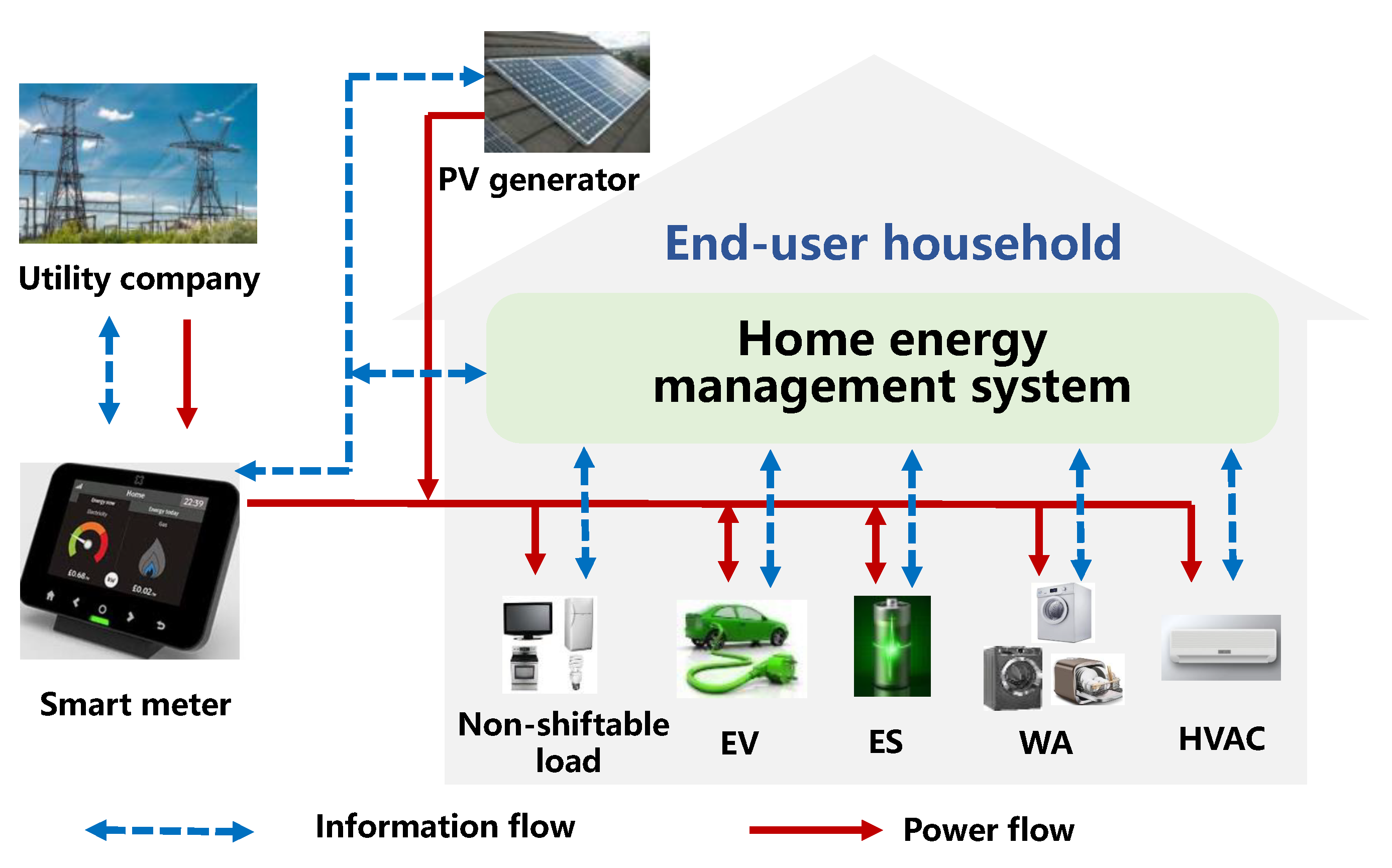
A Markov decision process (MDP) is constructed to formulate the optimal DR management problem for a residential household operating with multiple and diverse DERs, including PV generators, ES units, and three types of FD technologies, namely an EV with flexible charging and vehicle-to-grid (V2G)/vehicle-to-home (V2H) capabilities, wet appliances (WAs) with deferrable cycles, and HVAC with certain comfortable temperature margins.

-

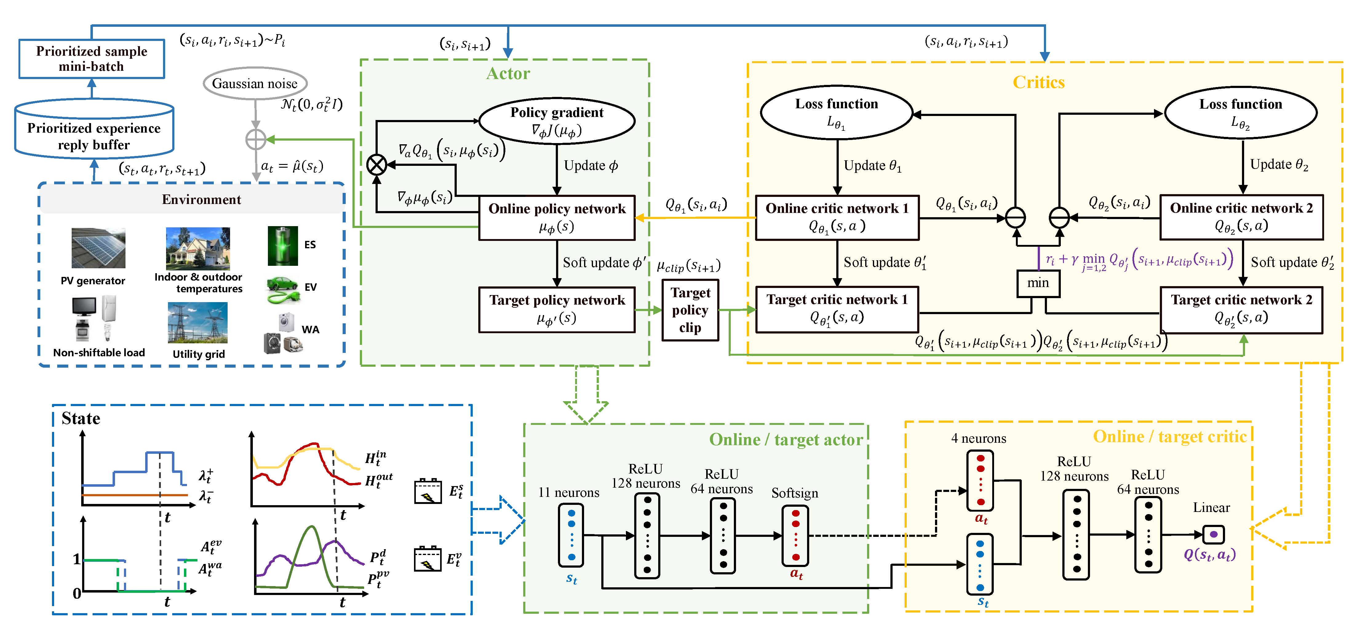
A model-free and data-driven approach based on TD3, which does not rely on any knowledge of the DERs’ operational models and parameters, is proposed to optimize the real-time DR management strategy. In contrast to previous works where the DR management problem was addressed by employing discrete control RL methods, the TD3 method allows learning of neural-network-based, fine-grained DR management policies in a multi-dimensional action space by harnessing high-dimensional sensory data that also encapsulate the system uncertainties.

-

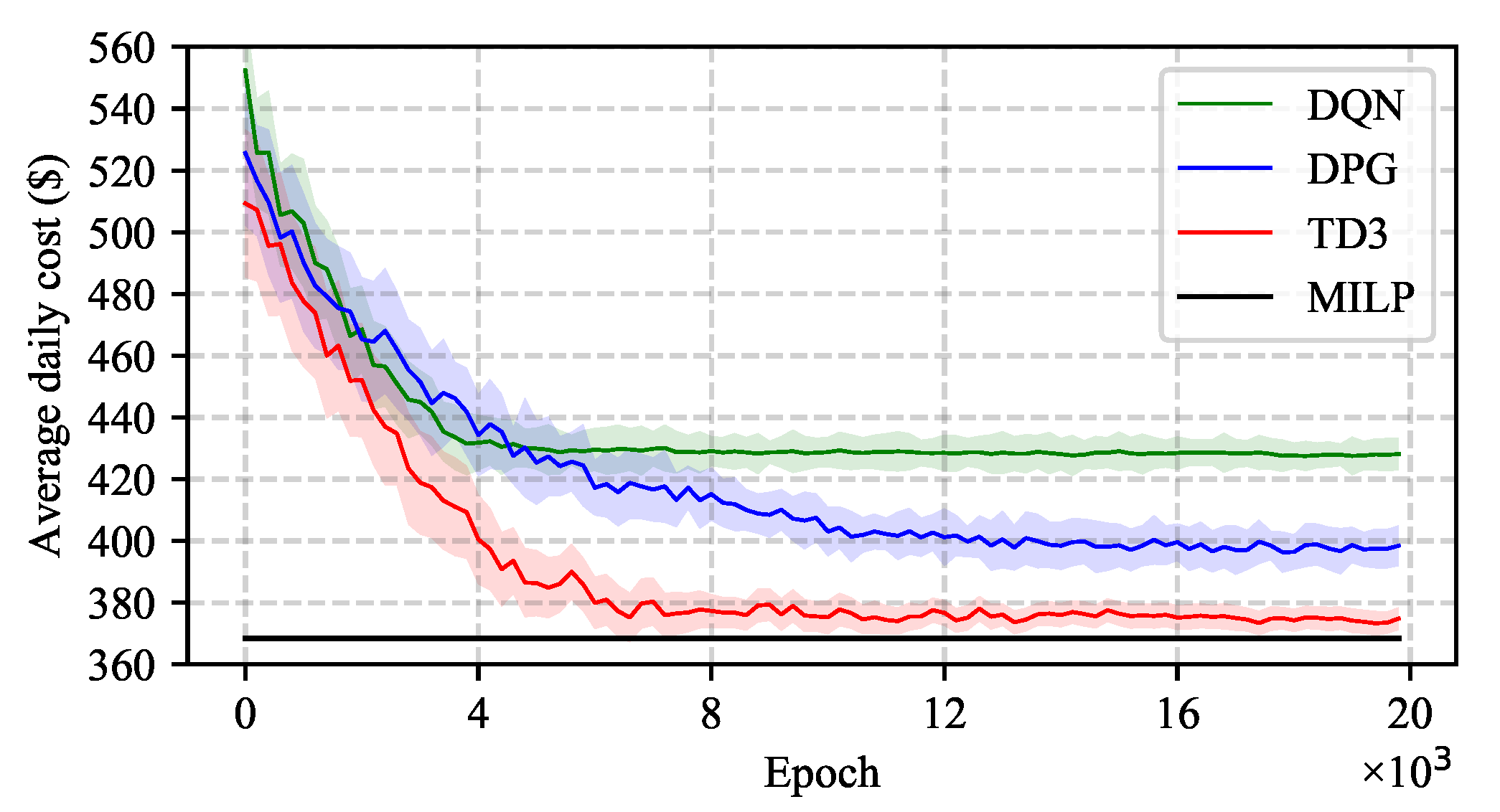
Case studies on a real-world scenario substantiate the superior performance of the proposed method in being more computationally efficient, as well as in achieving a significantly lower daily energy cost than the state-of-the-art DRL methods, while coping with the uncertainties stemming from both the electricity prices and the supply and demand sides of an end-user’s DERs.

1.4. Paper Organization

The rest of the paper is structured as follows. Section 2 presents the system model and problem formulation. Section 3 details the proposed TD3-based DR management algorithm, and its effectiveness is verified with simulation results in Section 4. Finally, Section 5 discusses the conclusions of this work.

2. System Model and Problem Formulation

The investigated residential household with an HEMS managing a portfolio of assorted DERs is shown in Figure 1. The installation of an on-site, non-dispatchable PV generator and an integrated ES unit can supply the household’s electricity demand in addition to acquiring some revenue by selling surplus PV power to the grid. The appliances of a household can generally be separated into two categories: non-shiftable and shiftable. The shiftable appliances can be further sub-categorized as interruptible and non-interruptible. The power demand of the non-shiftable appliances (e.g., lighting loads) must be supplied by the HEMS without any delay when they are active. On the other hand, the HEMS can delay the consumption of the shiftable appliances. WAs (e.g., washing machine, dishwasher, tumble dryer), or deferrable appliances, constitute the most representative types of the non-interruptible appliances. Their load cycles are flexible in scheduling within a specific time window but cannot be interrupted or altered. In contrast, EVs and HVAC are characterized as interruptible appliances whose operation times and energy usage can be flexibly adjusted upon satisfying some specific operating constraints, e.g., the traveling energy requirement constraint for an EV and the comfortable indoor temperature range constraint for  HVAC.

The HEMS is assumed to operate in slotted time steps, i.e., $t\in [1,T]$ with a temporal resolution $\Delta t$ = 0.5 h, where T = 48 is the total number of time steps in an investigated day. At each time step, the HEMS manages the charging and/or discharging power of the EV, ES, WAs, and HAVC based on high-dimensional sensory data comprised of the non-shiftable load, PV generation, outdoor temperature, the state of charge of the ES and EV, and the utility buy/sell prices, aiming at minimizing the daily energy cost of the household while maintaining a comfortable indoor temperature range. Next, we present the operating models of the EV, ES, WAs, and HVAC, as well as the model-based daily cost minimization problem for their management.

2.1. Electric Vehicle (EV) and Energy Storage (ES)

The EV is flexible in terms of the time periods in which it can acquire the amount of energy needed for its operation, as long as this is completed within a scheduling interval allowed by its users. In addition, the EV can inject stored energy during this interval (i.e., it exhibits V2G/V2H capabilities). The charging/discharging power of the EV can be continuously regulated between 0 and a maximum level, and it needs to fulfill an energy requirement for the envisaged journeys within the scheduling interval (with grid connection). Each EV is assumed to depart from its grid connection point only once within the horizon of the coordination problem (at step $t^{dep}$) and subsequently arrive back at its grid connection point only once during the same horizon (at step $t^{arr}$). The operating model of the EV includes the following constraints:

Constraint (1) corresponds to the EV battery’s energy balance, taking into account the energy needed for commuting purposes as well as the losses caused by charging and discharging efficiencies.

$$E_{t+1}^{ev}=E_t^{ev}+P_t^{evc}\Delta t{\eta }^{evc}-P_t^{evd}\Delta t/{\eta }^{evd}-E_t^{tr},\forall t$$

(1)

Constraint (2) expresses the lower and upper bounds of the battery’s energy content.

$$E^{ev,min}\le E_t^{ev}\le E^{ev,max},\forall t$$

(2)

Constraints (3)–(4) represent the limits of the battery’s charging/discharging power, which depends on its power capacity $P^{ev,max}$ and on if the EV is available for scheduling ($A_t^{ev}=1$) or not ($A_t^{ev}=0$), while the binary variable $V_t^{ev}$ is employed to avoid simultaneous charging and discharging.

$$0\le P_t^{evc}\le V_t^{ev}{A}_t^{ev}{P}^{ev,max},\forall t$$

(3)

$$0\le P_t^{evd}\le (1-V_t^{ev})A_t^{ev}{P}^{ev,max},\forall t\forall t$$

(4)

Finally, constraint (5) ensures that the EV is sufficiently charged upon departure to satisfy the commuting requirements of its users.

$$E_{t^{dep}}^{ev}\ge \sum _t{E}_t^{tr}$$

(5)

The operating model of the ES [39] is similar to that of the EV apart from the fact that the traveling energy requirement $E_t^{tr}$ and the scheduling availability $A_t^{ev}$ are irrelevant and are thus removed.

2.2. Wet Appliances (WAs)

The operation of WAs is based on the execution of user-prescribed cycles, which comprise a sequence of sub-processes occurring in a fixed sequence with a generally fixed duration and fixed power demand, which are immutable [40]. Their flexibility is measured by the ability to defer these cycles up to a maximum delay limit set by their users. Without loss of generality, each WA is assumed to be activated for one operational cycle per day by its users only once during the temporal horizon between the cycle’s earliest initiation time $t^{in}$ and latest termination time $t^{ter}$. The operating model of the WAs includes the following constraints:

Constraint (6) ensures that the demand activity of the WAs can be carried out once at most during the time window determined by $t^{in}$ and $t^{ter}$.

$$\sum _{t=t^{in}}^{t^{ter}-T^{dur}+1}{V}_t^{wa}=1$$

(6)

Constraint (7) expresses that the power demand of the WAs at each time step is dependent on the initiation time, $A_t^{wa}$, $T^{dur}$, and $P_{\tau }^{cyc},\forall \tau \in [1,T^{dur}]$.

$$P_t^{wa}=\sum _{\tau =1}^{T^{dur}}{V}_{t+1-\tau }^{wa}{A}_t^{wa}{P}_{\tau }^{cyc},\forall t$$

(7)

2.3. Heating, Ventilation, and Air Conditioning (HVAC)

The flexibility of the examined HVAC systems lies in that an indoor temperature range can be specified by the users so that their thermal comfort is preserved. The representation of the thermal comfort is a non-trivial task, as it depends on many diverse factors (e.g., air temperature, mean radiant temperature, relative humidity, air speed, etc.). Following the practice of [41], a comfortable temperature range is employed as the representation of thermal comfort:

$$H^{min}\le H_t^{in}\le H^{max},\forall t$$

(8)

Equation (9) represents the dynamic thermal behavior of the heated/cooled space, following the first-order model presented in [41]:

$$H_{t+1}^{in}=H_t^{in}-(H_t^{in}-H_t^{out}+{\eta }^{hvac}{R}^{hvac}{P}_t^{hvac})\Delta t/\left(C^{hvac}{R}^{hvac}\right),\forall t$$

(9)

where $C^{hvac}$ and $R^{hvac}$ are, respectively, the thermal capacity and resistance of the heated/cooled space. ${\eta }^{hvac}$ is the energy efficiency of HVAC; this value is positive for cooling and negative for heating.

Equation (10) expresses the electric power limits of the HVAC system:

$$0\le P_t^{hvac}\le P^{hvac,max},\forall t$$

(10)

2.4. Daily Energy Cost Minimization

The net demand (positive)/generation (negative) $l_t$ of the household at step t can be expressed as:

$$l_t=P_t^d-P_t^{pv}+P_t^{evc}-P_t^{evd}+P_t^{esc}-P_t^{esd}+P_t^{wa}+P_t^{hvac}$$

(11)

Finally, the daily energy cost minimization problem for the household can be formulated as:

$$\min \sum _{t=1}^T{C}_t$$

(12)

$$\mathrm{where}{C}_t={\lambda }_t^{+}{\left[l_t\right]}^{+}+{\lambda }_t^{-}{\left[l_t\right]}^{-}$$

(13)

$$\mathrm{s}.\mathrm{t}.\left(1\right)-\left(11\right)$$

(14)

where operators ${[·]}^{+/-}=max/min\{·,0\}$ indicate taking the maximum/minimum value between · and 0. The first term in (12) represents the cost of purchasing electricity from the grid, while the second term represents the revenue from selling excess PV production, ES, and EV discharge to the grid.

Note that problems (12)–(14) are a mixed-integer linear program (MILP) that provides a model-based DR management strategy that aims to minimize the daily energy cost, assuming full knowledge of the operating models and parameters of all the DERs and a perfect prediction of all the uncertain parameters. As such, the optimal cost in (12) can be treated as a lower bound on the cost (since the uncertainties are completely neglected), which later provides a theoretical baseline for the model-free DRL DR management strategy. As discussed in Section 1.2, the SP approach is computationally inefficient in optimizing the DR management strategy while dealing with the multi-source system uncertainties. To address this, we propose an alternative approach for addressing the real-time DR management problem.

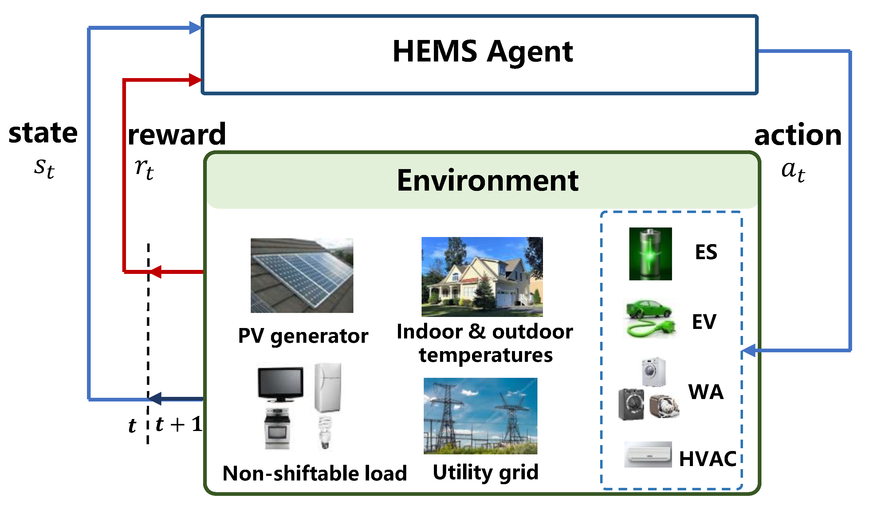
3. DR Management as an MDP

A finite Markov decision process (MDP) with discrete time steps is applied to formulate the real-time DR management problem. The time interval between two adjacent time steps is 30 min (the proposed approach can be readily extended to employ a finer temporal resolution). The HEMS constitutes the agent, while the environment is composed of many objects outside the agent (e.g., utility company, PV generator, non-shiftable loads, ES, EV), as shown in Figure 2. In the context of RL, an agent acts in an environment by sequentially taking actions over a sequence of time steps to maximize a cumulative reward. In general, RL can be described as an MDP that includes: (1) a state space $\mathcal{S}$; (2) an action space $\mathcal{A}$; (3) a transition dynamics distribution with conditional transition probability $p\left(s_{t+1}\right|s_t,a_t)$, which models the uncertainty in the evolution of states of the environment based on the executed actions of the agent; and (4) a reward r: $\mathcal{S}\times \mathcal{A}\to \mathbb{R}$. The detailed MDP formulation for the DR management problem is detailed below.

(1) State: The state $s_t$ at step t received by the HEMS agent entails the influence of its action on the status of the environment. $s_t$ is identified as an 11-dimensional vector $s_t=[t,{\lambda }_t^{+},{\lambda }_t^{-},H_t^{out},H_t^{in},P_t^d,P_t^{pv},E_t^{ev},E_t^{es},A_t^{ev},A_t^{wa}]\in \mathcal{S}$, which comprises the following sensory information: the time step identifier t; the utility buy price ${\lambda }_t^{+}$ and sell price ${\lambda }_t^{-}$; the outdoor $H_t^{out}$ and indoor $H_t^{in}$ temperatures; the non-shiftable demand $P_{i,t}^d$; the PV production $P_t^{pv}$; the energy content of the EV $E_t^{eV}$ and ES $E_t^{eS}$; and the EV’s $A_t^{ev}$ and WAs’ $A_t^{wa}$ scheduling availability indicators.

(2) Action: The action $a_t$ at step t encompasses its employed management decisions for the controllable DERs (including the EV, ES, WAs, and HVAC). It is defined as $a_t=[a_t^{ev},a_t^{es},a_t^{wa},a_t^{hvac}]\in \mathcal{A}$, where $a_t^{ev}$ and $a_t^{es}\in [-1,1]$ represent the size of the charging (positive) and discharging (negative) power of the EV and ES as a percentage of $P^{ev,max}$ and $P^{es,max}$, $a_t^{wa}=V_t^{wa}\in \{0,1\}$ represents whether the cycle of the WAs is initiated ($a_t^{wa}=1$) or not ($a_t^{wa}=0$) at step t, and $a_t^{hvac}$ represents the magnitude of the input power of the HVAC as a ratio of $P^{hvac,max}$.

After the execution of action $a_t$, the environment maps $a_t$ to the respective power output/input of each DER and subsequently determines the next state $s_{t+1}$ and reward $r_t$. Based on the EV operating model presented in Section 2.1, mutually exclusive quantities $P_{i,t}^{evc}$ and $P_{i,t}^{evd}$ (as EVs cannot charge and discharge at the same time step) are managed by action $a_t^{ev}$, and are also limited by the EV’s parameters $A_t^{ev}$, $E_t^{ev}$, $E^{ev,min}$, $E^{ev,max}$, ${\eta }^{evc}$, and ${\eta }^{evd}$.

$$P_t^{evc}=\min \left(a_t^{ev}{A}_t^{ev}{P}^{ev,max},(E^{ev,max}-E_t^{ev})/({\eta }^{evc}\Delta t)\right)$$

(15)

$$P_t^{evd}=\min \left(-a_t^{ev}{A}_t^{ev}{P}^{ev,max},(E_t^{ev}-E^{ev,min}){\eta }^{evd}/\Delta t\right)$$

(16)

Based on $P_t^{evc}$ and $P_t^{evd}$, the energy context of the EV battery at the next time step $E_{i,t+1}^{ev}$ can be written as (17).

$$E_{t+1}^{ev}=E_t^{ev}+P_t^{evc}\Delta t{\eta }^{evc}+P_t^{evd}\Delta t/{\eta }^{evd}-E_t^{tr}$$

(17)

Quantities $P_t^{esc},P_t^{esd},$ and $E_{t+1}^{es}$ can be obtained following the ES operating model (Section 2.1) and the same logic of the above derivation for (15)–(17), but they neglect the charging availability.

Based on the WA operating model presented in Section 2.2, the power demand of the WAs $P_t^{wa}$ is managed by action $a_t^{wa}$, and is also affected by the WA parameters $T^{dur}$, $A_t^{wa}$, and $P_{\tau }^{cyc},\forall \tau \in [1,T^{dur}]$.

$$P_t^{wa}={\sum }_{\tau =1}^{T^{dur}}{a}_{t+1-\tau }^{wa}{A}_t^{wa}{P}_{\tau }^{cyc}$$

(18)

Finally, on the basis of the HVAC operating model in Section 2.3, the indoor temperature at the next time step $H_{t+1}^{in}$ based on $P_t^{hvac}$ can be expressed as:

$$H_{t+1}^{in}=H_t^{in}-(H_t^{in}-H_t^{out}+{\eta }^{hvac}{R}^{hvac}{a}_t^{hvac}{P}^{hvac,max})\Delta t/\left(C^{hvac}{R}^{hvac}\right)$$

(19)

(3) Reward: Since the objective of the HEMS agent is to minimize the total energy cost of the household while maintaining a comfortable indoor temperature as well as ensuring the satisfaction of all DERs’ operating constraints, the reward function is designed to include the following three components:

1) $r_t^{cost}$, which is as the negative total energy cost of the household:

$$r_t^{cost}=-C_t=-({\lambda }_t^{+}{\left[l_t^n\right]}^{+}+{\lambda }^{-}{\left[P_t^n\right]}^{-})$$

(20)

2) $r_t^{com}$, which serves as a penalty for indoor temperature deviation from a desirable range, with ${\kappa }_1$ denoting a positive weighting factor:

$$r_t^{com}={\kappa }_1({[H_t^{in}-H^{max}]}^{+}+{[H^{min}-H_t^{in}]}^{+})$$

(21)

3) $r_t^{pen}$, which serves as a penalty for the constraint violations of the DERs, with ${\kappa }_2$ denoting a positive weighting factor:

$$r_t^{pen}=\left\{\begin{array}{cc}-{\kappa }_2{[E_t^{ev}-{\sum }_t{E}_t^{tr}]}^{+},\hfill & \mathrm{if}t=t^{dep}\hfill \\ -{\kappa }_2|{\sum }_{t=t^{in}}^{t^{ter}-T^{dur}+1}{a}_t^{wa}-1|,\hfill & \mathrm{if}t=t_i^{ter}-T^{dur}+1\hfill \end{array}\right.$$

(22)

Note that in (15)–(16), the charging and discharging power of the EV only respects the minimum/maximum power and energy limits of the EV, but does not ensure that its state-of-charge level is sufficient to cover the energy requirements for traveling, i.e., constraint (5) may not be satisfied. Furthermore, constraint (6) should be satisfied at the last initiation step to ensure the daily activation frequency of the WAs. To adequately account for these inter-temporal constraints of the EV and WAs, we introduce a penalty term $r_t^{pen}$ in the reward function.

The final reward function $r_t$ can be expressed as:

$$r_t=r_{i,t}^{cost}+r_t^{com}+r_t^{pen}$$

(23)

(4) Performance and value functions: The agent employs a policy $\pi$ to interact with the MDP and emit a trajectory of states, actions, and rewards: $s_1,a_1,r_1,s_2,a_2,r_2,\dots$ over $\mathcal{S}\times \mathcal{A}\times \mathbb{R}$. The agents’ objective is to learn a policy that maximizes the cumulative discounted reward from the start state $s_1$, which is termed as the performance function $J\left(\pi \right)=\mathbb{E}\left[R_1|\pi \right]={\mathbb{E}}_{s\sim {\rho }^{\pi },a\sim \pi }\left[r\right]$, where ${\rho }^{\pi }$ denotes the discounted state distribution and $R_t={\sum }_{l=t}^T{\gamma }^{(l-t)}{r}_l$ is the discounted reward, where $\gamma \in [0,1]$ is the discount factor. Furthermore, the Q-value function $Q^{\pi }(s,a)=\mathbb{E}\left[R_1|s_1=s,a_1=a;\pi \right]$ forms an estimation of the discounted reward given an action a at state s and following the policy $\pi$ from the succeeding states onwards.

4. Proposed TD3-Based DR Management Strategy

As discussed in Section 1.2, despite the popularity of applying QL and DQN for DR management problems in the existing literature, they both suffer, to some extent, from the curse of dimensionality driven by their need to discretize the state and/or the action spaces. Furthermore, the discretization may hinder the decision-making process of the HEMS agent, leading to sub-optimal DR management policies. The DPG method is criticized for its low sampling efficiencies and high variance in its gradient estimator. In order to address these challenges, the proposed DR management strategy is founded on the TD3 method [38], the overall workflow of which is presented in Figure 3. TD3 leverages the performance of the state-of-the-art DRL method for continuous control, i.e., DDPG.

TD3 features an actor–critic architecture, which employs (a) a parameterized critic network $Q_{\theta }$ that inputs a state $s_t$ and action $a_t$ and outputs an estimate of the Q-value function $Q_{\theta }(s_t,a_t)$ and (b) a parameterized actor network ${\mu }_{\varphi }$ that inputs a state $s_t$ and implements a policy improvement task that updates the policy with respect to the estimated Q-value function and outputs a continuous action ${\mu }_{\varphi }\left(s_t\right)$. QL and DQN both feature a greedy maximization of the Q-value function concerning policy improvement, i.e., $\mu \left(s_{t+1}\right)=arg{max}_{a_{t+1}}Q(s_{t+1},a_{t+1})$. However, such a greedy strategy exhibits significant intractability in the high-dimensional continuous action domain, since the Q-value function needs to be globally maximized at every step. Instead, TD3 utilizes the actor $\mu$ to produce an action ${\mu }_{\varphi }\left(s_{t+1}\right)$ for the next state. The critic is responsible for policy evaluation, or criticizing the policy obtained by the actor by generating a Q-value estimate with temporal difference (TD) learning. This is achieved by minimizing the following regression loss function:

$$L_{\theta }=\mathbb{E}\left[{\left(r_t+\gamma Q_{\theta }\left(s_{t+1},{\mu }_{\varphi }\left(s_{t+1}\right)\right)-Q_{\theta }(s_t,a_t)\right)}^2\right]$$

(24)

where $r_t+\gamma Q_{\theta }\left(s_{t+1},\mu \left(s_{t+1}\right)\right)$ denotes the target Q-value at step t. Instead of globally maximizing $Q_{\theta }(s_t,a_t)$, the critic evaluates the gradients ${\nabla }_a{Q}_{\theta }(s_t,a_t)$, which indicate the directions for the change of action to purse higher estimated Q-values. As a result, the weights of the actor are updated in the direction of the performance gradient ${\nabla }_{\varphi }J\left({\mu }_{\varphi }\right)$, which is derived according to the deterministic policy gradient theorem [42]:

$$\begin{array}{c}\hfill {\nabla }_{\varphi }J\left({\mu }_{\varphi }\right)={\mathbb{E}}_{s\sim {\rho }^{\mu }}\left[{\nabla }_a{Q}_{\theta }(s,a){|}_{a={\mu }_{\varphi }\left(s\right)}{\nabla }_{\varphi }{\mu }_{\varphi }\left(s\right)\right].\end{array}$$

(25)

Exploration vs. exploitation: Maintaining an effective trade-off between exploration and exploitation plays a vital role in effective RL learning. To aid the agent in exploring the environment thoroughly, an exploration/behavior policy $\widehat{\mu }\left(s_t\right)$ is constructed, which imposes a random Gaussian noise ${\mathcal{N}}_t(0,{\sigma }_t^{2}I)$ on the actor’s output ${\mu }_{\varphi }\left(s_t\right)$:

$$\widehat{\mu }\left(s_t\right)={\mu }_{\varphi }\left(s_t\right)+{\mathcal{N}}_t(0,{\sigma }_t^{2}I).$$

(26)

It is well recognized that RL’s learning process tends to exhibit instability or even divergence when a DNN is employed as a nonlinear regressor for the Q-value function. To tackle such instability, previous works have put forward two tailored mechanisms.

Target Networks: Observe in (24) that the online network $Q_{\theta }$ is utilized for both the current Q-value estimation $Q_{\theta }(s_t,a_t)$ and the target Q-value $r_t+\gamma Q_{\theta }(s_{t+1},{\mu }_{\varphi }\left(s_{t+1}\right))$. As a consequence, the Q-value update is prone to oscillations. To remedy this instability, a target network [26] can be introduced for the actor and critic, denoted as ${\mu }_{{\varphi }^{\prime }}\left(s_t\right)$ and $Q_{{\theta }^{\prime }}(s_t,a_t)$, respectively. They are only used for evaluating the target values. Furthermore, the weights of these target networks can be updated by having them gradually track the weights of the online networks as ${\theta }^{\prime }\leftarrow \upsilon \theta +(1-\upsilon ){\theta }^{\prime }$ with $\upsilon \ll 1$. Similarly to the idea of temporally freezing the Q-target value during training (in DQN), but modified for the actor–critic RL method, the rationale behind the soft update is to restrict the target values (for both actor and critic) to change slowly for an enhanced learning stability.

Experience Replay: Since the experiences are sequentially generated through the agent’s interaction with the environment, there exists temporal correlation in these experiences, which can degrade machine learning models substantially. The employment of an experience replay buffer $\mathcal{B}$ [26] resolves this challenge. It is a cache that pools the past experiences and uniformly samples a minibatch for training the actor and critic. Mixing recent with previous experiences alleviates the temporal correlations of the sampled experiences. Furthermore, it enables samples to be reused, which enhances the sampling efficiency.

Despite the remarkable success that DDPG has received in various power system and smart grid applications, it is often criticized for the overestimation bias of the Q-value functions, which can result in sub-optimal policies [38]. TD3 is tailored to address this challenge by concurrently learning two Q-value functions instead of one.

Double Critic Networks: In RL methods focusing on learning the Q-value, such as QL and DQN, function approximation errors may arise, which can result in an overestimated Q-value and, consequently, sub-optimal policies [43,44]. Concretely, the target Q-values used by QL and DQN can be written as:

$$y^{QL}=r_t+\gamma Q\left(s_{t+1},arg\underset{a_{t+1}}{max}Q(s_{t+1},a_{t+1})\right)$$

(27)

$$y^{DQN}=r_t+\gamma Q_{{\theta }^{\prime }}\left(s_{t+1},arg\underset{a_{t+1}}{max}{Q}_{{\theta }^{\prime }}(s_{t+1},a_{t+1})\right)$$

(28)

It can be observed that QL uses the same Q-table both to select (in the $argmax$ operator) and to evaluate (calculate the target Q-value, which is subsequently used in the Q-value update) an action. Analogously, DQN uses the same set of neural network weights ${\theta }^{\prime }$ to both select and evaluate an action. This renders it more likely to select overestimated Q-values, leading to overoptimistic value estimates. Furthermore, such an overestimation bias can be propagated in time through the Bellman equation and can be developed into a more significant bias after many updates if left unnoticed. In the case of DDPG, since the policy ${\mu }_{\varphi }$ is optimized with respect to the critic $Q_{\theta }$, using the same estimate in the target update of $Q_{\theta }$ can create a similar overestimation of $Q_{\theta }$. This may adversely affect the policy quality, since sub-optimal actions may be highly rated by a sub-optimal critic, reinforcing the selection of these actions in the subsequent policy updates.

To address the drawback of using a single Q-value estimator, we propose a variant of the Double $QL$ method [43] and adopt it in the actor–critic setting in order to mitigate the risk of having an overestimated Q-value. To achieve this, we introduce two independently trained online critic networks $(Q_{{\theta }_1},Q_{{\theta }_2})$ and their corresponding target networks $\left(Q_{{\theta }_1^{\prime }},Q_{{\theta }_2^{\prime }}\right)$. It is assumed that $Q_{{\theta }_1}/Q_{{\theta }_2}$ are the potentially biased/less biased Q-value estimates, respectively. Since a Q-value estimate that suffers from overestimation bias can be used as an approximated upper bound for the true value estimate, we use $Q_{{\theta }_1}$ as the upper bound of $Q_{{\theta }_2}$. Equivalently, this is results in taking the minimum between these two estimates to get the target Q-value:

$$y=r_{\tau }+\gamma \underset{j=1,2}{min}{Q}_{{\theta }_j^{\prime }}\left(s_{\tau +1},{\mu }_{\mathrm{clip}}\left(s_{\tau +1}\right)\right)$$

(29)

Another potential failure in DDPG is that if the Q-function approximator develops an incorrect sharp peak for some actions, the policy will quickly overfit to such narrow peaks, leading to incorrect behavior. This can be averted by smoothing out the Q-function over similar actions, which target policy smoothing is designed to do. In this effect, actions used to form the critic target are based on the target policy ${\mu }_{{\varphi }^{\prime }},$ but with clipped noise added on each action dimension. After adding the clipped noise, the target action is clipped again to lie in the valid action range $[a_{\mathrm{Low}},a_{\mathrm{High}}]$. The target actions can be expressed as:

$${\mu }_{\mathrm{clip}}\left(s_{\tau +1}\right)=clip\left({\mu }_{{\varphi }^{\prime }}\left(s_{\tau +1}\right)+clip(ϵ,-b,b),a_{\mathrm{Low}},a_{\mathrm{High}}\right),ϵ\sim \mathcal{N}\left(0,{\sigma }^2\right)$$

(30)

As discussed previously, target networks can be used to reduce the error over multiple updates, while policy updates on states corresponding to high TD error may lead to divergent learning behavior. As a result, TD3 updates the policy network at a lower frequency than the critic network in order to sufficiently minimize error before introducing a policy update. In this effect, a modification is introduced only to update the policy and target networks after Z updates to the critic.

By incorporating the target network, experience replay, and the above-mentioned modifications, the critic loss in (24) can be stated as the weighted mean-squared TD error calculated based on the training data, i.e., a minibatch of prioritized sampled K experiences.

$$L_{{\theta }_j}=K^{-1}\sum _{k=1}^K{\delta }_{k,j}^2$$

(31)

where the TD error for each critic can be expressed as:

$${\delta }_{k,j}=r_{k,j}+\gamma \underset{j=1,2}{min}{Q}_{{\theta }_j^{\prime }}\left(s_{k+1,j}{\mu }_{\mathrm{clip}}\left(s_{k+1,j}\right)\right)-Q_{{\theta }_j}\left(s_{k,j}{a}_{k,j}\right)$$

(32)

The policy gradient for the actor update in (25) can be restated in a similar fashion:

$${\nabla }_{\varphi }J\left({\mu }_{\varphi }\right)={\left.K^{-1}\sum _{k=1}^K{\nabla }_a{Q}_{{\theta }_1}\left(s_{k,1},a\right)\right|}_{a={\mu }_{\varphi }\left(s_{k,1}\right)}{\nabla }_{\varphi }{\mu }_{\varphi }\left(s_{k,1}\right)$$

(33)

Finally, the following updates are applied to the weights of the online critic networks:

$${\theta }_j\leftarrow {\theta }_j-{\alpha }^{\theta }{\nabla }_{{\theta }_j}{L}_{{\theta }_j}$$

(34)

and after Z learning steps, the online actor and the target networks are updated according to:

$$\varphi \leftarrow \varphi -{\alpha }^{\varphi }{\nabla }_{\varphi }J\left({\mu }_{\varphi }\right)$$

(35)

$${\theta }_j^{\prime }\leftarrow \upsilon {\theta }_j+(1-\upsilon ){\theta }_j^{\prime }\mathrm{and}{\varphi }^{\prime }\leftarrow \upsilon \varphi +(1-\upsilon ){\varphi }^{\prime }$$

(36)

where ${\alpha }^{\theta }$ and ${\alpha }^{\varphi }$ are the learning rates of the gradient descent algorithm and $\upsilon$ is the soft update rate.

Algorithm 1 details the training of the DNNs employed by TD3, and the proposed TD3-based DR management strategy is outlined in Algorithm 2. After the training phase, we firstly load the weight of the online actor network that is trained by Algorithm 1. For a specific test day, at each time step t, the agent observes the current environment state $s_t$ and determines its DR management action according to the policy learned by TD3. The requested DR actions are then mapped to the input/output of different DERs of the household (Section 3).

Algorithm 1 Training procedure of TD3

1: Initialize critic networks $Q_{{\theta }_1}$ and $Q_{{\theta }_2}$ and actor network ${\mu }_{\varphi }$ with random weights ${\theta }_1$, ${\theta }_2$, and $\varphi$. 2: Initialize target networks with weights ${\theta }_1^{\prime }\leftarrow {\theta }_1,{\theta }_2^{\prime }\leftarrow$${\theta }_2$, and ${\varphi }^{\prime }\leftarrow \varphi$. 3: for episode (i.e., day) $e=1:E^{train}$ do 4:   Obtain the initial state $s_1$ from the training set. 5:   Initialize a random Gaussian exploration noise ${\mathcal{N}}_t$. 6:   for time step (i.e., 30 min) $t=1:T$ do 7:     The HEMS agent selects action $a_t$ using (26). 8:     Execute $a_t$ in the environment, observe $r_t$ using (23), and transit to the new state $s_{t+1}$ 9:     Store $\left(s_t,a_t,r_t,s_{t+1}\right)$ in the experience replay buffer. 10:     Sample a minibatch K of experiences from reply buffer. 11:     Compute target actions ${\mu }_{\mathrm{clip}}\left(s_{\tau +1}\right)$ using (30). 12:     Update the online critics using (34). 13:     if $\tau modZ$ then then 14:       Update the online actor using (35). 15:       Update the target networks using (36). 16:      end if 17:    end for 18: end for

Algorithm 2 TD3-based DR management strategy

1: Load the DNN parameter ${\varphi }^{*}$ of the online actor network ${\mu }_{{\varphi }^{*}}$ trained by Algorithm 1. 2: for test day = $1:E^{test}$ do 3:   Obtain the initial state $s_1$ of the test day. 4:   for time step = $1:T$ do 5:     Set the DR management action as $a_t={\mu }_{{\varphi }^{*}}\left(s_t\right)$. 6:     Execute action $a_t$ in the environment, calculate reward $r_t$, and transit to the new state $s_{t+1}$. 7:    end for 8: end for

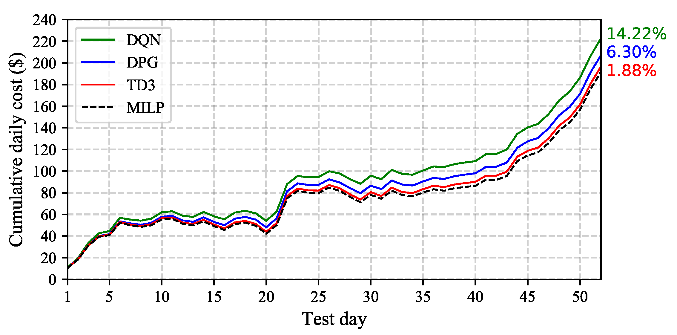
5. Results and Discussion

5.1. Simulation Setup and Implementation

The proposed TD3-based DR management strategy was trained and tested on a real-world scenario using household solar PV and non-shiftable load data published by Ausgrid, Australia. The employed data were collected from 1 June 2012 to 31 May 2013 (53 weeks) with a half-hourly resolution. The data for household outdoor temperature were collected from open Australian government database [45].

The assumed operating parameters of the EV, ES, WAs, and HVAC were derived from [41,46] and are provided in

Table 2. Operating parameters for the electric vehicle (EV), energy storage (ES), wet appliances (WAs), and heating, ventilation, and air conditioning (HVAC).

EV		ES		WA		HVAC
Parameter	Value	Parameter	Value	Parameter	Value	Parameter	Value
$T^{dur}$ (h)	2	$H^{min},H^{max}$ (°C) *	19, 24	$E^{es.max}$ (kWh)	10	$E^{ev.max}$ (kWh)	15
$P_1^{cyc}$ (kW)	0.56	$C^{hvac}$ (kWh/°F)	0.33	$E^{es,min}$ (kWh)	2	$E^{ev,min}$ (kWh)	3
$P_2^{cyc}$ (kW)	0.56	$R^{hvac}$ (°F/kW)	13.5	$E^{es,max}$ (kWh)	10	$E^{ev,max}$ (kWh)	15
$P_3^{cyc}$ (kW)	0.63	${\eta }^{hvac}$	2.2	${\eta }^{esc}/{\eta }^{esd}$	0.95	${\eta }^{evc}/{\eta }^{evd}$	0.93
$P_4^{cyc}$ (kW)	0.63	$P^{hvac,max}$ (kW)	1.75	$P^{es,max}$ (kW)	4	$P^{ev,max}$ (kW)	6

* °F = °C * 1.8 + 32.

. Concretely, it was assumed that an EV user makes two trips per day; each is defined by a departure time, an arrival time, and an energy requirement. The grid connection period of the EV was assumed to be between the end of the second and the start of its first trip. In order to capture the inherent uncertainty residing in the DERs’ operating models, the following parameters were modeled as random variables: the EV departure and arrival times, the energy requirements, the initial energy level in the EV and ES batteries, the earliest initiation and latest termination times of the WAs, and the initial indoor temperature of the HVAC. To this end, we employed truncated normal distribution $\mathcal{TN}$ for parameters related to temperature and energy and discrete uniform distribution for parameters related to time, as detailed in

Table 3. Distributions of the operating parameters of the EV, ES, WAs, and HVAC.

Parameter	Distribution
$E_0^{ev}$ (kWh)	$\mathcal{TN}(9,1^2,6,12)$
$E_0^{es}$ (kWh)	$\mathcal{TN}(6,1^2,4,8)$
$E^{tr}$ (kWh)	$\mathcal{TN}(7.12,{0.712}^2,5.696,8.544)$
$t^{dep}$	$\mathcal{TN}(8,1^2,6,10)$
$t^{arr}$	$\mathcal{TN}(18,1^2,16,20)$
$t^{in}$	$\mathcal{TN}(21,1^2,19,23)$
$t^{ter}$	$\mathcal{TN}(7,1^2,5,9)$
$T_0^{in}$ (°C)	$\mathcal{TN}(21,1^2,19,24)$

.

In the simulations, we uniformly picked one day from each of the 53 weeks to form the test set and used the rest of days as the training set. The utility buy price data follow the time-of-use structure provided in [45], partitioned into summer and winter periods, while the utility sell price is fixed at 0.04 AUD/kWh [47] throughout the year.

The TD3 algorithm employed two DNNs (i.e., online and target) for the actor and the two critics. The Adam optimizer [48] was used for learning the neural network weights with learning rates of ${\alpha }^{\varphi }={10}^{-4}$ and ${\alpha }^{\theta }={10}^{-3}$ for the actor and critics, respectively. A soft update rate of $\nu ={10}^{-3}$ was used. A discount factor of $\gamma =0.99$ was used for the critics. As shown in Figure 3, the actor and the critics all had two hidden layers with 128 and 64 neurons, respectively. Both the actor and critic employed rectified non-linearity (ReLU) [49] for all hidden layers. The output layer of the actor was a softsign layer [50] to bound the continuous actions. The minibatch size and the replay buffer size were set as 128 and ${10}^5$, respectively. All investigated coordination methods were implemented in Python. The training process of the examined learning algorithms was carried out on a computer with a four-core 2.80 GHz Intel(R) Core(TM) i7-7700HQ CPU and 16 GB of RAM, and the total training time for TD3 was 949 s.

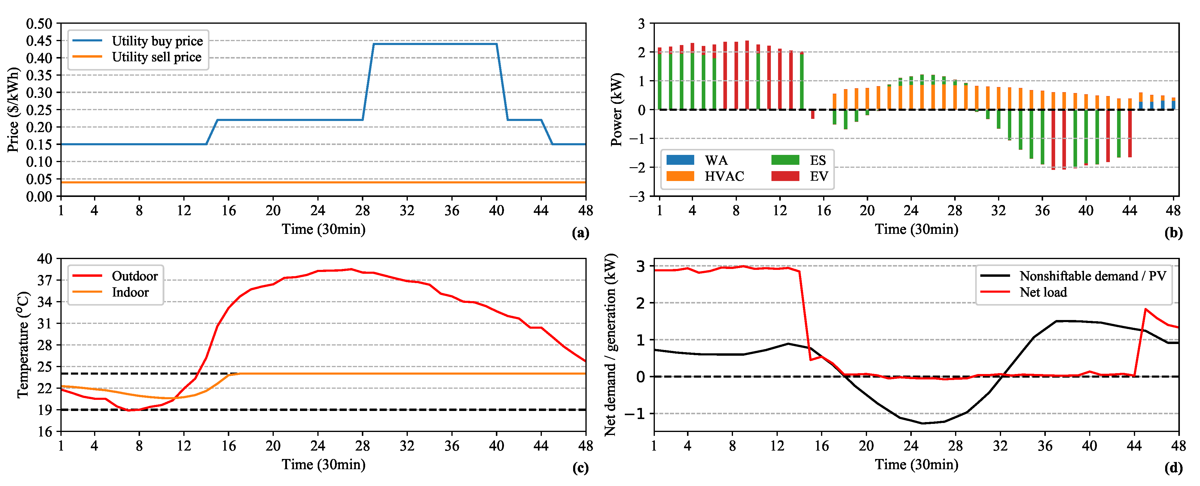
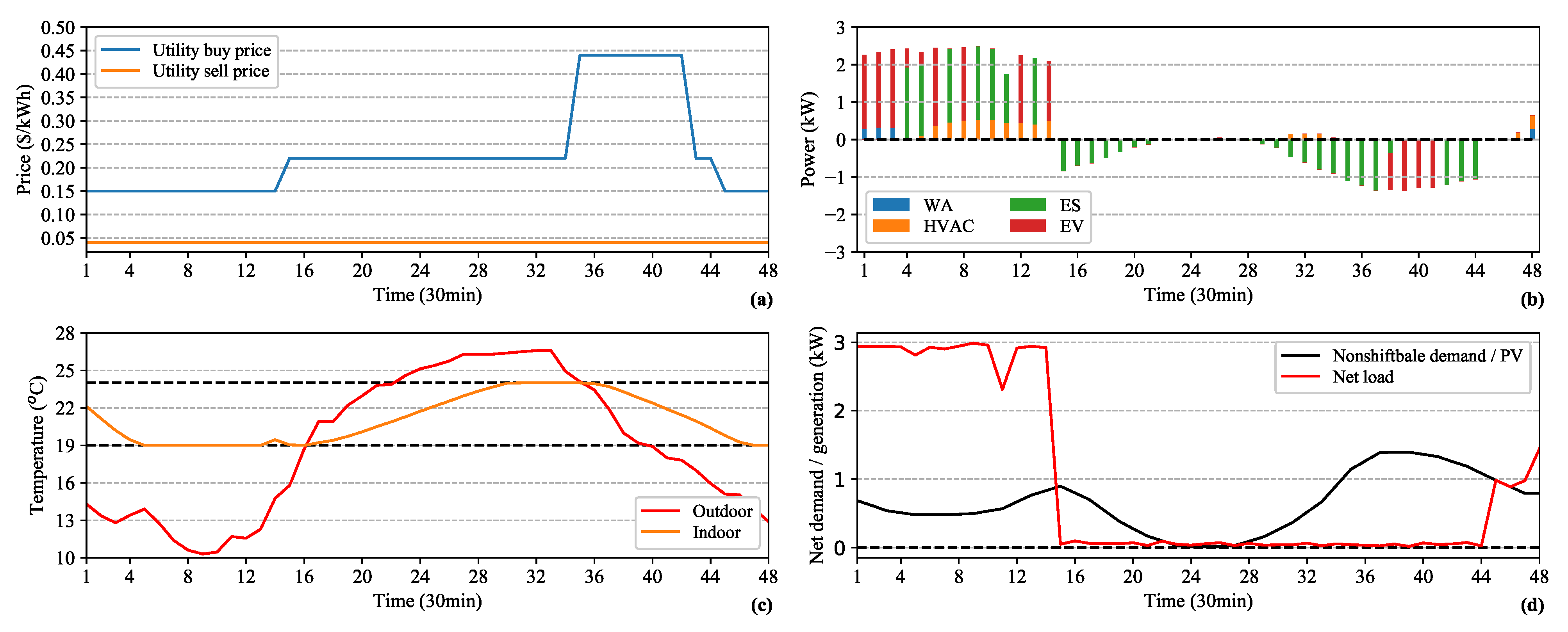
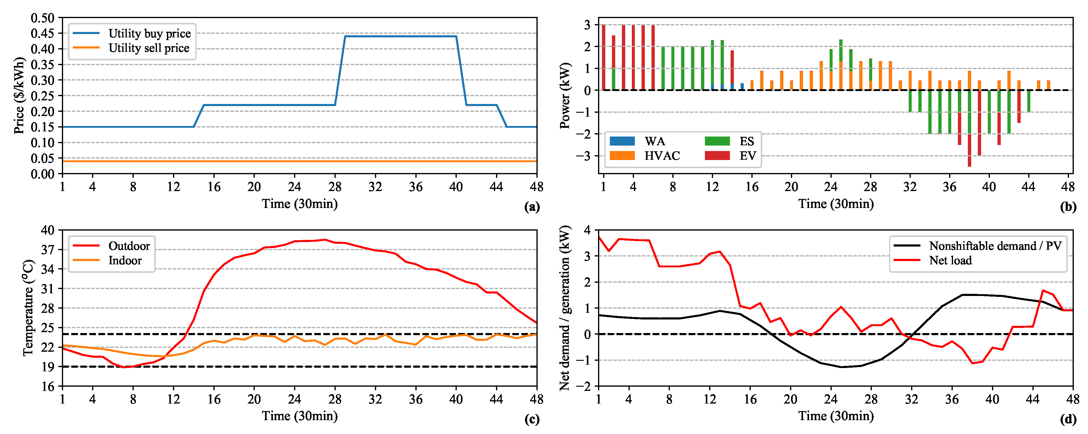
5.2. Performance Evaluation

We benchmarked the performance of TD3 with DQN and DPG (which are widely adopted in the existing literature on DR management problems, as discussed in Section 1.2) in order to validate its performance superiority. Furthermore, we solved the daily cost minimization problem (MILP) presented in Section 2.4 and calculated the average daily energy cost over the 53 test days (as depicted by the black horizontal line in Figure 4). In this case, ${\overline{C}}^{*}=$ 368 cents can be regarded as the theoretical optimal solution of the investigated DR management problem. In other words, it represents a lower bound on the daily cost, indicating how far from the optimum the DRL-based DR management strategy is.

To assess the average performance as well as the variability of the examined DRL-based methods, 10 different random seeds were generated, and each DRL method was trained for 20,000 epochs for each seed. Each epoch signifies a random day selected from the training dataset consisting of 48 time steps. During training, the cost effectiveness of the learned DR strategy was evaluated on the test dataset every 200 epochs. Figure 4 depicts the average daily cost $\overline{C}$ (over the 53 test days) for the investigated DRL methods with 10 random seeds. The mean and the standard deviation of the average daily cost over the 10 seeds are displayed by solid curves and shaded areas, respectively, in Figure 4. The cumulative daily energy costs of the 53 test days under TD3 and all examined baseline methods are presented in Figure 5.

As observed in Figure 4, TD3 improves the cost effectiveness of its DR management policy gradually with a declining standard deviation. Ultimately, only TD3 converges to a near-optimal solution. TD3 exhibits superior performance with regard to the two baseline DRL methods, exhibiting the lowest average daily cost of 374 cents (only 1.85% above the theoretical optimum ${\overline{C}}^{*}$) and achieving the lowest standard deviation of 4 cents at convergence. In relative terms, TD3 outperforms DQN and DPG with 12.45%/5.93% lower average daily cost and 29.35%/44.50% lower standard deviation, respectively. In addition, it is evident that the continuous DR management strategy (employing TD3 and DPG) is more cost effective than the discrete one (employing DQN), since the former enables the agent to discover more a fine-grained DR management strategy in a multi-dimensional continuous action space. A more comprehensive illustration of the value of the continuous DR management strategy is presented in Section 5.3. Going further, TD3 exhibits superior convergence performance with respect to DPG in terms of the obtained average daily cost and learning stability. This superior performance is attributed to TD3’s higher sampling efficiency in computing the policy gradient as well as the policy evaluation enabled by the joint learning of the critic in addition to the policy. On the contrary, DPG features no policy evaluation, contributing to high variance in its policy gradient estimation. Furthermore, TD3 updates the actor and critics in an online manner (i.e., the updates are performed on every time step), whereas a trajectory of experiences must be obtained before an update of the policy network can be introduced in DPG. Finally, TD3 incorporates tailored mechanisms to mitigate the overestimation of the Q-value functions, evading erroneous convergence to sub-optimal policies and thereby improving the convergence performance. As depicted in Figure 5, the cumulative costs obtained by the two benchmark approaches, DQN (green solid curve) and DPG (blue solid curve), are 14.22% and 6.30% higher than the theoretical optimum, respectively. In comparison, the cumulative cost under TD3 (red solid curve) is only 1.88% higher than the theoretical optimum (black dashed curve).

To further elaborate on the generalization capability of the learned DR management policies of TD3 with respect to the system uncertainties, we investigated the obtained DR schedules of the household for a representative summer and winter day selected from the 53 test days (reflecting the seasonable variations in the utility price, PV generation, and outdoor temperature), as displayed in Figure 6 and Figure 7, respectively.

The summer day (Figure 6) features ample PV generation and high outdoor temperature. At the beginning of the day, the HEMS learns not to operate the HVAC system to conserve energy and reduce cost, since the outdoor temperature is relatively low but is well above the minimum comfortable temperature (19 °C). A surge in the outdoor temperature is observed at around 5:00. As a result, the indoor temperature also increases (with a time lag) and the HVAC system is only scheduled to be on when the indoor temperature reaches the maximum comfortable temperature (24 °C) at around 8:00. During the mid-day periods (9:00–16:00), the operation of the HVAC system is optimized such that it can absorb a significant portion of the plentiful PV generation during these periods while maintaining the indoor temperature marginally below 24 °C in order to minimize cost. Furthermore, the HEMS also learns to absorb the PV generation by charging the ES instead of selling it to the grid because the utility buy price during the mid-day periods is still higher than the unfavorable sell price. During peak periods (17:00–22:00) where the PV generation is absent, it is observed that the peak demand is sufficiently flattened by discharging the ES and EV (which are both scheduled to charge during the cheapest off-peak periods). As observed in Figure 6, the learned DR management policy contributes 13 h (from 9:00–22:00) with net zero cost in total by optimally scheduling the complementary DERs and harnessing their flexibility potentials.

The winter day (Figure 7) is distinguished by scarce PV generation and low outdoor temperature. At the beginning of the day, the outdoor temperature is significant lower than the minimum comfortable temperature; the HEMS adapts to this exogenous condition by turning on the HVAC system for heating and conservatively scheduling it to sustain the indoor temperature marginally above 19 °C. After 8:00, accompanied by the increase of the utility buy price (Figure 7a), the HEMS learns to turn off the HVAC system to save cost. Subsequently, it is observed that the indoor temperature varies (with a time delay) with the outdoor temperature until the end of the day without operating the HVAC system. Similarly to the trend observed in Figure 6, the HEMS learns to charge the ES and EV sufficiently during the off-peak periods and discharge them in the morning (8:00–10:00) and afternoon/evening (14:00–22:00) peak demand periods, leading to a total of 14 h with net zero cost.

It can be concluded that the learned DR management policy exhibits excellent generalization performance with respect to the seasonal and daily variations associated with the utility prices, PV generation, residential demand, and outdoor temperature. Furthermore, the obtained DR management policies enable comprehensive harnessing of the flexibility value of complementary DERs, thus promising efficient utilization of RESs and substantial cost savings for the end-user.

5.3. Benefits of Continuous DR Management

This section more deeply explores the physical significance of the continuous DR management strategy enabled by TD3 by comparing it to DQN (a commonly employed discrete DRL method in this research topic). For DQN’s implementation, actions $a_t^{ev}$ and $a_t^{es}$ are discretized in five integer values representing charging or discharging levels of 0%, 50%, and 100% of the maximum power limits of the EV and ES. Actions $a_t^{hvac}$ is also discretized in five integer values representing a power demand of 0%, 25%, 50%, 75%, and 100% of the maximum power input of the HVAC. Figure 8 illustrates the DR schedules of the household obtained using DQN for the same summer day as that examined in the previous section.

Driven by the employed discretization of actions, the power input and/or output of the HVAC, EV, and ES can only be adjusted in discrete blocks, as mentioned above. In the case of the HVAC system, its demand profile is characterized by lumpiness, which exhibits significant fluctuations with respect to the one observed in Figure 6b, since the HEMS can now only adjust the power input of HVAC in five discrete blocks. This, in turn, leads to the fluctuations in the indoor temperature. In the case of the EV, since its charging power can no longer be continuously regulated, the HEMS charges the EV more during the off-peak period in order to guarantee the fulfillment of its traveling energy requirement. In the case of ES, owning to the lumpiness of the HVAC demand during the mid-day periods, the HEMS charges the ES more during these periods in order to fully consume the PV generation. However, since the power output of the PV generator is not controllable, this inevitably leads to purchasing of superfluous electricity (i.e., overcharging of ES) at high utility buy prices (Figure 8a). As a consequence of the charging activities of the EV and ES, significant reverse power flow (from selling excessive EV and ES discharges to the gird) is witnessed during the peak demand periods. Overall, the EV and ES are scheduled to charge at the shoulder/peak utility buy price and are discharged at the unfavorable utility sell price (0.04 AUD/kWh), resulting in non-economical operation. Overall, the daily energy cost under DQN (465 cents) is approximately 24.33% higher than the one under TD3 (374 cents). It can therefore be concluded that discrete control DRL methods hinder the comprehensive exploitation of the flexibility potential offered by DERs as well as the coordinated scheduling of complementary DERs.

6. Conclusions

In this paper, we formulate a real-time demand response management problem for a residential household as a Markov decision process. In the problem formulation, the uncertainties stemming from the supply (photovoltaic generation), demand (non-shiftable load, electric vehicle, wet appliances, heating, ventilation, and air conditioning), and storage (electric storage and electric vehicle) sides of the end-users are taken into account. A model-free and data-driven deep-reinforcement-learning-based demand response management strategy whose performance does not rely on accurate mathematical modeling of the distributed energy resources’ operating models or the uncertainties was developed to determine the real-time control strategies for the household. The proposed approach constitutes an extension of the state-of-the-art deep deterministic policy gradient learning algorithm by addressing its overestimation error in the Q-value function, thus avoiding sub-optimal policies and promising better convergence properties. In comparison to the commonly employed Q-learning and deep Q network discrete control reinforcement learning methods, the proposed approach enables the agent to learn more fine-grained demand response management policies from high-dimensional sensory data. Case studies employing a large-scale real-world dataset have offered numerous valuable insights around the significance of the proposed demand response management strategy. The simulation results demonstrated that the twin delayed deep deterministic policy gradient manages to converge to a near-optimal solution and reduces the energy cost by approximately 12.45% and 5.93% compared to the costs obtained by using the deep Q network and deep policy gradient, respectively. Furthermore, the proposed method enables a representation of real-time and cost-effective demand response management strategies to be constructed, and these are shown to be generalizable despite the variabilities in multiple uncertain parameters of the problem.

References

1. Shakoor, A.; Davies, G.; Strbac, G. Roadmap for Flexibility Services to 2030; A report to the Committee on Climate Change; Pöyry: London, UK, 2017. [Google Scholar]
2. O’Connell, A.; Taylor, J.; Smith, J.; Rogers, L. Distributed Energy Resources Takes Center Stage: A Renewed Spotlight on the Distribution Planning Process. IEEE Power Energy Mag. 2018, 16, 42–51. [Google Scholar] [CrossRef]
3. Pedrasa, M.A.A.; Spooner, T.D.; MacGill, I.F. Coordinated scheduling of residential distributed energy resources to optimize smart home energy services. IEEE Trans. Smart Grid 2010, 1, 134–143. [Google Scholar] [CrossRef]
4. Bozchalui, M.C.; Hashmi, S.A.; Hassen, H.; Canizares, C.A.; Bhattacharya, K. Optimal operation of residential energy hubs in smart grids. IEEE Trans. Smart Grid 2012, 3, 1755–1766. [Google Scholar] [CrossRef]
5. Rastegar, M.; Fotuhi-Firuzabad, M. Load management in a residential energy hub with renewable distributed energy resources. Energ. Build. 2015, 107, 234–242. [Google Scholar] [CrossRef]
6. Moghaddam, I.G.; Saniei, M.; Mashhour, E. A comprehensive model for self-scheduling an energy hub to supply cooling, heating and electrical demands of a building. Energy 2016, 94, 157–170. [Google Scholar] [CrossRef]
7. Basit, A.; Sidhu, G.A.S.; Mahmood, A.; Gao, F. Efficient and autonomous energy management techniques for the future smart homes. IEEE Trans. Smart Grid 2017, 8, 917–926. [Google Scholar] [CrossRef]
8. Chen, Z.; Wu, L.; Fu, Y. Real-time price-based demand response management for residential appliances via stochastic optimization and robust optimization. IEEE Trans. Smart Grid 2012, 3, 1822–1831. [Google Scholar] [CrossRef]
9. Shafie-Khah, M.; Siano, P. A stochastic home energy management system considering satisfaction cost and response fatigue. IEEE Trans. Ind. Inform. 2017, 14, 629–638. [Google Scholar] [CrossRef]
10. Huang, Y.; Wang, L.; Guo, W.; Kang, Q.; Wu, Q. Chance constrained optimization in a home energy management system. IEEE Trans. Smart Grid 2016, 9, 252–260. [Google Scholar] [CrossRef]
11. Yu, L.; Jiang, T.; Zou, Y. Online energy management for a sustainable smart home with an HVAC load and random occupancy. IEEE Trans. Smart Grid 2017, 10, 1646–1659. [Google Scholar] [CrossRef] [Green Version]
12. Du, Y.F.; Jiang, L.; Li, Y.; Wu, Q. A robust optimization approach for demand side scheduling considering uncertainty of manually operated appliances. IEEE Trans. Smart Grid 2016, 9, 743–755. [Google Scholar] [CrossRef] [Green Version]
13. Birge, J.R.; Louveaux, F. Introduction to Stochastic Programming, 2nd ed.; Springer: New York, NY, USA, 2011. [Google Scholar]
14. Bertsimas, D.; Brown, D.B.; Caramanis, C. Theory and applications of robust optimization. SIAM Rev. 2011, 53, 464–501. [Google Scholar] [CrossRef]
15. Liang, Y.; He, L.; Cao, X.; Shen, Z.J. Stochastic control for smart grid users with flexible demand. IEEE Trans. Smart Grid 2013, 4, 2296–2308. [Google Scholar] [CrossRef]
16. Wen, Z.; O’Neill, D.; Maei, H. Optimal demand response using device-based reinforcement learning. IEEE Trans. Smart Grid 2015, 6, 2312–2324. [Google Scholar] [CrossRef] [Green Version]
17. Remani, T.; Jasmin, E.; Ahamed, T.I. Residential load scheduling with renewable generation in the smart grid: A reinforcement learning approach. IEEE Syst. J. 2019, 12, 3283–3294. [Google Scholar] [CrossRef]
18. Berlink, H.; Kagan, N.; Costa, A.H.R. Intelligent decision-making for smart home energy management. J. Intell. Robot. Syst. 2015, 80, 331–354. [Google Scholar] [CrossRef]
19. Guan, C.; Wang, Y.; Lin, X.; Nazarian, S.; Pedram, M. Reinforcement learning-based control of residential energy storage systems for electric bill minimization. In Proceedings of the 12th Annual IEEE Consumer Communications and Networking Conference (CCNC), Las Vegas, NV, USA, 9–12 January 2015; pp. 637–642. [Google Scholar]
20. Kim, S.; Lim, H. Reinforcement learning based energy management algorithm for smart energy buildings. Energies 2018, 11, 2010. [Google Scholar] [CrossRef] [Green Version]
21. Wang, H.; Zhang, B. Energy storage arbitrage in real-time markets via reinforcement learning. In Proceedings of the 2018 IEEE Power & Energy Society General Meeting (PESGM), Portland, OR, USA, 5–10 August 2018; pp. 1–5. [Google Scholar]
22. Ruelens, F.; Claessens, B.J.; Vandael, S.; De Schutter, B.; Babuška, R.; Belmans, R. Residential demand response of thermostatically controlled loads using batch reinforcement learning. IEEE Trans. Smart Grid 2017, 8, 2149–2159. [Google Scholar] [CrossRef] [Green Version]
23. Claessens, B.J.; Vrancx, P.; Ruelens, F. Convolutional neural networks for automatic state-time feature extraction in reinforcement learning applied to residential load control. IEEE Trans. Smart Grid 2018, 9, 3259–3269. [Google Scholar] [CrossRef] [Green Version]
24. Ruelens, F.; Claessens, B.J.; Quaiyum, S.; De Schutter, B.; Babuška, R.; Belmans, R. Reinforcement learning applied to an electric water heater: From theory to practice. IEEE Trans. Smart Grid 2018, 9, 3792–3800. [Google Scholar] [CrossRef] [Green Version]
25. Wu, D.; Rabusseau, G.; François-lavet, V.; Precup, D.; Boulet, B. Optimizing Home Energy Management and Electric Vehicle Charging with Reinforcement Learning. In Proceedings of the 16th Adaptive Learning Agents (ALA), Stockholm, Sweden, 10–15 July 2018; pp. 1–8. [Google Scholar]
26. Mnih, V.; Kavukcuoglu, K.; Silver, D.; Rusu, A.A.; Veness, J.; Bellemare, M.G.; Graves, A.; Riedmiller, M.; Fidjeland, A.K.; Ostrovski, G.; et al. Human-level control through deep reinforcement learning. Nature 2015, 518, 529–533. [Google Scholar] [CrossRef]
27. Mocanu, E.; Mocanu, D.C.; Nguyen, P.H.; Liotta, A.; Webber, M.E.; Gibescu, M.; Slootweg, J.G. On-line building energy optimization using deep reinforcement learning. IEEE Trans. Smart Grid 2019, 10, 3698–3708. [Google Scholar] [CrossRef] [Green Version]
28. Tsang, N.; Cao, C.; Wu, S.; Yan, Z.; Yousefi, A.; Fred-Ojala, A.; Sidhu, I. Autonomous Household Energy Management Using Deep Reinforcement Learning. In Proceedings of the 25th IEEE International Conference on Engineering, Technology and Innovation (ICE/ITMC), Valbonne Sophia-Antipolis, France, 17–19 June 2019; pp. 1–7. [Google Scholar]
29. Wan, Z.; Li, H.; He, H.; Prokhorov, D. Model-Free Real-Time EV Charging Scheduling Based on Deep Reinforcement Learning. IEEE Trans. Smart Grid 2019, 10, 5246–5257. [Google Scholar] [CrossRef]
30. François-Lavet, V.; Taralla, D.; Ernst, D.; Fonteneau, R. Deep reinforcement learning solutions for energy microgrids management. In Proceedings of the European Workshop on Reinforcement Learning (EWRL 2016), Barcelona, Spain, 3–4 December 2016; pp. 1–7. [Google Scholar]
31. Chen, T.; Su, W. Local Energy Trading Behavior Modeling With Deep Reinforcement Learning. IEEE Access 2018, 6, 62806–62814. [Google Scholar] [CrossRef]
32. Ji, Y.; Wang, J.; Xu, J.; Fang, X.; Zhang, H. Real-Time Energy Management of a Microgrid Using Deep Reinforcement Learning. Energies 2019, 12, 2291. [Google Scholar] [CrossRef] [Green Version]
33. Wei, T.; Wang, Y.; Zhu, Q. Deep reinforcement learning for building hvac control. In Proceedings of the 54th Annual Design Automation Conference 2017, Austin, TX, USA, 18–22 June 2017; pp. 1–7. [Google Scholar]
34. Lillicrap, T.P.; Hunt, J.J.; Pritzel, A.; Heess, N.; Erez, T.; Tassa, Y.; Silver, D.; Wierstra, D. Continuous control with deep reinforcement learning. In Proceedings of the 4th International Conference Learning Represent (ICLR), San Juan, Puerto Rico, 2–4 May 2016; pp. 1–14. [Google Scholar]
35. Konda, V.R.; Tsitsiklis, J.N. Actor-critic algorithms. In Proceedings of the Advances in Neural Information Processing Systems, Denver, CO, USA, 3–8 December 2000; pp. 1008–1014. [Google Scholar]
36. Wan, Z.; Li, H.; He, H. Residential energy management with deep reinforcement learning. In Proceedings of the 2018 International Joint Conference on Neural Networks (IJCNN), Rio de Janeiro, Brazil, 8–13 July 2018; pp. 1–7. [Google Scholar]
37. Ye, Y.; Qiu, D.; Wu, X.; Strbac, G.; Ward, J. Model-Free Real-Time Autonomous Control for A Residential Multi-Energy System Using Deep Reinforcement Learning. IEEE Trans. Smart Grid 2020, 11, 3068–3082. [Google Scholar] [CrossRef]
38. Fujimoto, S.; Van Hoof, H.; Meger, D. Addressing function approximation error in actor-critic methods. In Proceedings of the Machine Learning Research, New York, NY, USA, 23–24 February 2018. [Google Scholar]
39. Ye, Y.; Papadaskalopoulos, D.; Moreira, R.; Strbac, G. Investigating the impacts of price-taking and price-making energy storage in electricity markets through an equilibrium programming model. IET Gener. Transm. Distrib. 2018, 13, 305–315. [Google Scholar] [CrossRef]
40. Ye, Y.; Papadaskalopoulos, D.; Strbac, G. Factoring flexible demand non-convexities in electricity markets. IEEE Trans. Power Syst. 2014, 30, 2090–2099. [Google Scholar] [CrossRef] [Green Version]
41. Du, Y.; Jiang, L.; Duan, C.; Li, Y.; Smith, J. Energy consumption scheduling of HVAC considering weather forecast error through the distributionally robust approach. IEEE Trans. Ind. Inf. 2017, 14, 846–857. [Google Scholar] [CrossRef] [Green Version]
42. Silver, D.; Lever, G.; Heess, N.; Degris, T.; Wierstra, D.; Riedmiller, M. Deterministic policy gradient algorithms. In Proceedings of the 31st International Conference on Machine Learning (ICML), Beijing, China, 21–26 June 2014; pp. 1–9. [Google Scholar]
43. Hasselt, H.V. Double Q-learning. In Proceedings of the Advances in Neural Information Processing Systems, Vancouver, BC, Canada, 6–9 December 2010; pp. 2613–2621. [Google Scholar]
44. Van Hasselt, H.; Guez, A.; Silver, D. Deep reinforcement learning with double q-learning. In Proceedings of the 30th AAAI Conference on Artificial Intelligence, Phoenix, AZ, USA, 12–17 February 2016. [Google Scholar]
45. Ratnam, E.L.; Weller, S.R.; Kellett, C.M.; Murray, A.T. Residential load and rooftop PV generation: An Australian distribution network dataset. Int. J. Sustain. Energy 2017, 36, 787–806. [Google Scholar] [CrossRef]
46. Papadaskalopoulos, D.; Strbac, G. Nonlinear and randomized pricing for distributed management of flexible loads. IEEE Trans. Smart Grid 2016, 7, 1137–1146. [Google Scholar] [CrossRef] [Green Version]
47. EnergyAustralia. Solar Rebates and Feed-in Tariffs; EnergyAustralia: Melbourne, VIC, Australia, 2020. [Google Scholar]
48. Kingma, D.P.; Ba, J. Adam: A method for stochastic optimization. In Proceedings of the 3rd International Conference Learning Represent (ICLR), Diego, CA, USA, 7–9 May 2015; pp. 1–15. [Google Scholar]
49. Glorot, X.; Bordes, A.; Bengio, Y. Deep sparse rectifier neural networks. In Proceedings of the 14th Conference Artificial Intelligence and Statistics (AISTATS), Fort Lauderdale, FL, USA, 11–13 April 2011; pp. 315–323. [Google Scholar]
50. Bergstra, J.; Desjardins, G.; Lamblin, P.; Bengio, Y. Quadratic Polynomials Learn Better Image Features; Technical Report 1337; Dept. IRO, Université de Montréal: Montréal, QC, Canada, 2009. [Google Scholar]
Figure 1. Schematic representation of the investigated household operating multiple and diverse DERs.
Energies 14 00531 g001
Figure 2. Interactions between agent and environment in the Markov decision process (MDP).
Energies 14 00531 g002
Figure 3. Overall workflow of the proposed TD3-based DR management method.
Energies 14 00531 g003
Figure 4. Average daily cost evaluated over the test dataset for the examined deep reinforcement learning (DRL) methods with 10 different random seeds.
Energies 14 00531 g004
Figure 5. Cumulative daily costs of the twin delayed deep deterministic policy gradient (TD3) and all the baseline methods over the 53 test days.
Energies 14 00531 g005
Figure 6. (a) Utility buy and sell prices, (b) aggregated schedule of flexible DERs, (c) indoor and outdoor temperature, and (d) net demand/generation of the household with/without flexible DERs for the investigated summer day under the TD3 method.
Energies 14 00531 g006
Figure 7. (a) Utility buy and sell prices, (b) aggregated schedule of flexible DERs, (c) indoor and outdoor temperature, and (d) net demand/generation of the household with/without flexible DERs for the investigated winter day under the TD3 method.
Energies 14 00531 g007
Figure 8. (a) Utility buy and sell prices, (b) aggregated schedule of flexible DERs, (c) indoor and outdoor temperature, and (d) net demand/generation of the household with/without flexible DERs for the investigated summer day under the deep Q network (DQN) method.
Energies 14 00531 g008