Article

Linearized Frequency-Dependent Reflection Coefficient and Attenuated Anisotropic Characteristics of Q-VTI Model

1
School of Geosciences, China University of Petroleum (East China), Qingdao 266580, China
2
Department of Geological Science, The University of Alabama, Tuscaloosa, AL 35487, USA
3
School of Geophysics and Petroleum Resources, Yangtze University, Wuhan 430100, China
*
Author to whom correspondence should be addressed.
Energies 2021, 14(24), 8506; https://doi.org/10.3390/en14248506
Submission received: 9 November 2021 / Revised: 8 December 2021 / Accepted: 13 December 2021 / Published: 16 December 2021

Abstract

:
Seismic wave exhibits the characteristics of anisotropy and attenuation while propagating through the fluid-bearing fractured or layered reservoirs, such as fractured carbonate and shale bearing oil or gas. We derive a linearized reflection coefficient that simultaneously considers the effects of anisotropy and attenuation caused by fractures and fluids. Focusing on the low attenuated transversely isotropic medium with a vertical symmetry axis (Q-VTI) medium, we first express the complex stiffness tensors based on the perturbation theory and the linear constant Q model at an arbitrary reference frequency, and then we derive the linearized approximate reflection coefficient of P to P wave. It decouples the P- and S-wave inverse quality factors, and Thomsen-style attenuation-anisotropic parameters from complex P- and S-wave velocity and complex Thomsen anisotropic parameters. By evaluating the reflection coefficients around the solution point of the interface of two models, we analyze the characteristics of reflection coefficient vary with the incident angle and frequency and the effects of different Thomsen anisotropic parameters and attenuation factors. Moreover, we realize the simultaneous inversion of all parameters in the equation using an actual well log as a model. We conclude that the derived reflection coefficient may provide a theoretical tool for the seismic wave forward modeling, and again it can be implemented to predict the reservoir properties of fractures and fluids based on diverse inversion methods of seismic data.

1. Introduction

Development of seismic acquisition and processing technology makes it possible to sufficiently employ useful information embedded in seismic data, e.g., amplitude variation with offset, azimuth and frequency (AVO, AVAz, AVF), to estimate fluids and fractures. Recently, many studies revealed that seismic wave exhibit velocity dispersion and anisotropy while propagating in attenuated fractured media and attenuated finely layered media [1,2,3,4,5,6,7,8,9]. The seismic wave velocity dispersion refers to the phenomenon that the velocity varies with the frequency, and it accompanies with the seismic wave amplitude attenuation, which means amplitude decreases with the increase of distance. Therefore, the modeling of frequency-dependent attenuation and anisotropy of seismic waves, and the inversion for attenuation factors and anisotropic parameters using frequency-dependent seismic amplitude data, may help improve the reliability of the detection of fractured reservoirs and infilling fluids [10,11].
Under the assumption of static equivalent effective medium model, the rock physics models are employed to model how fractures induce the frequency-independent anisotropy, e.g., the linear slip model proposed by Schoenberg [12], the isolated fracture model of Hudson [13], the uniform pore model of Thomsen [1], and the model combining the linear slip model and anisotropic Gassmann equation proposed by Gurevich [14]. Meanwhile, Thomsen [1] demonstrates that the exchange of fluids between pores and fractures during the seismic wave propagation can affect the anisotropic elastic properties. On the other hand, dynamic equivalent medium models are proposed to describe how seismic wave propagates in fractured rocks in the case of considering the effect of frequency variation [2,3,4,5,6,7,8,9]. Typically, Chapman [15] proposed a model which considers coupled fluid motion on both the grain scale and fracture scale, which concludes that frequency-dependent anisotropy and strong anisotropic attenuation can occur in the seismic frequency band when large fractures are present, and it reveals that fracture and fluid properties can be estimated from frequency-dependent seismic data.
To model how the seismic amplitude varies with incident angle and frequency, we consider the effects of the parameters of anisotropy and attenuation on the reflection coefficient. Under the assumption of slight changes in properties across the reflection boundary, Aki and Richards [16] proposed linearized reflection coefficients which are the analytical solutions of the Zoeppritz equations. However, it is complicated to solve the Zoepprtitz equations that are extended to viscoelastic anisotropic media. Based on the Born approximation, Shaw and Sen [17] presented an approach to derive linearized reflection coefficients for arbitrary anisotropic media using the perturbation in stiffness matrix of anisotropic media. Following them, Zong [18] derived the seismic wave scattering coefficient in terms of P-wave and S-wave quality factors in a viscoelastic medium, Moradi and Innanen [19,20] derived the expressions for scattering potentials of PP wave and proposed a frequency-independent linearized reflection coefficient in the attenuated VTI medium. Chen [21,22] presented a linearized azimuthal and frequency-dependent PP-wave reflection coefficient in terms of dry rock elastic properties, dry fracture weaknesses and a new indicator of oil-bearing fractured reservoirs. Pan [23] used Born formalism and first-order perturbation assumption to derive a matrix-fluid-fracture decoupled-based linearized PP-wave reflection coefficient for a fluid-saturated fractured porous medium.
In the present study, we focus on the case of Q-VTI medium with low-loss attenuation and weak anisotropy, which means we neglect the term proportional to higher orders of the attenuation factors and Thomsen anisotropic parameters, and we let P-wave, SV-wave and SH-wave propagate in the linear constant Q attenuation reference media. We express the PP wave scattering potentials and derive the linearized frequency-dependent reflection coefficient for the Q-VTI medium. Utilizing the reflection coefficients, we analyze the variation of reflection coefficients with the incident angle and angular frequency in two reservoir models, and we also model how the attenuation factors and Thomsen anisotropic parameters affect the reflection coefficients. We conclude that, combining the rock physics effective model, the derived reflection coefficient may provide a theoretical tool to model how pore-, fracture-, and fluid-related parameters (e.g., porosity, fracture density, fluid modulus) affect the seismic wave amplitude, and can also be employed to estimate these parameters from incident angel- and frequency-dependent seismic data.

2. Theories and Methods

2.1. Approximation of Frequency-Dependent Complex Stiffness Tensors for Q-VTI Model

Seismic wave velocity in viscoelastic media is expressed as a function of v 0 , a phase velocity at an arbitrary reference frequency ω 0 , and Q , a quality factor describing absorption and attenuation. Kjartansson [24] derives the complex and frequency-dependent phase velocity v ˜ based on the linear constant Q model as,
v ˜ ( ω ) = v 0 ( i ω ω 0 ) 1 π Q 1 ,
where, the accent mark ‘~’ indicates the complex velocity in viscoelastic medium. Using Equation (1), the quality factor is computed as Q = v ˜ Re / v ˜ Im , where v ˜ Re and v ˜ Im are the real and imaginary parts of the complex velocity v ˜ .
We approximate the complex velocity using the Maclaurin series expansion of the exponential function, and preserve the first two terms of the expansion. The complex velocity is given by,
v ˜ ( ω ) v 0 [ 1 + 1 π Q 1 ln ( i ω ω 0 ) ] .
Similar to the derived approximate complex velocity, we express the complex stiffness tensor c ˜ I J as,
c ˜ I J ( ω ) = c I J 0 [ 1 + 2 π Q I J 1 ln ( i ω ω 0 ) ] ,
where, c I J 0 is the elastic stiffness tensor at an arbitrary reference frequency ω 0 , and Q I J 1 is the corresponding inverse quality factors.
A consistent description of P-wave property in VTI medium with weak anisotropy is given in terms of Thomsen anisotropic parameters [25,26]. For Q-VTI media, the complex Thomsen parameters are given by,
ε ˜ = c ˜ 11 c ˜ 33 2 c ˜ 33 γ ˜ = c ˜ 66 c ˜ 44 2 c ˜ 44 δ ˜ = ( c ˜ 13 + c ˜ 44 ) 2 ( c ˜ 33 c ˜ 44 ) 2 2 c ˜ 33 ( c ˜ 33 c ˜ 44 )
where, the Thomsen-style attenuation-anisotropic parameters ε Q , γ Q and δ Q are given by Zhu and Tsvankin [27,28] as,
ε Q = Q 11 1 Q 33 1 Q 33 1 γ Q = Q 66 1 Q 44 1 Q 44 1 δ Q = ( Q 13 1 + Q 44 1 ) 2 ( Q 33 1 Q 44 1 ) 2 2 Q 33 1 ( Q 33 1 Q 44 1 )
The parameters ε Q and γ Q represent the difference between the horizontal and vertical attenuation coefficients of P- and SH-waves, respectively, however, δ Q is defined through the second derivative of the P-wave attenuation coefficient in the symmetry direction, which refers to the coupling between the attenuation and velocity anisotropy.
We stress that in this study we consider the Q-VTI medium with constant attenuation and weak anisotropy (i.e., | ε | ,   | δ | ,   | γ | 1 ), which means the second and higher orders of quality factors and Thomsen parameters are neglected in the approximation process of the complex tensors. Consequently, the components of frequency-dependent complex stiffness tensor c ˜ I J ( ω ) are expressed in terms of two inverse quality factors, three Thomsen anisotropy parameters and corresponding Thomsen-style attenuation-anisotropic parameters,
c ˜ 11 = ρ v p 2 ( 1 + 2 ε ) + ρ v p 2 Q p 1 ( 1 + 2 ε + ε Q ) I ω c ˜ 13 = ρ v p 2 ( 1 + δ ) 2 c 55 + ρ v p 2 Q p 1 ( 1 + δ + δ Q ) I ω 2 ρ v s 2 Q s 1 I ω c ˜ 33 = ρ v p 2 + ρ v p 2 Q p 1 I ω c ˜ 55 = ρ v s 2 + ρ v s 2 Q s 1 I ω c ˜ 66 = ρ v s 2 ( 1 + 2 γ ) + ρ v s 2 Q s 1 ( 1 + 2 γ + γ Q ) I ω
where, I ω = 2 π ln ω ω 0 + i . The approximate results above decouple the effective factors from the complex tensors and distinguish the real and imaginary parts, elasticity and attenuation parameters.

2.2. Approximation of Frequency-Dependent Reflection Coefficient for Q-VTI Model

A scattering model of seismic wave interaction in an attenuated anisotropic medium is shown in Figure 1, which consists of a homogeneous reference medium and perturbations described by eleven properties. Taking density as an example, the term Δ ρ = ρ ρ 0 in Figure 1, represents the perturbation in density, which represents the difference between the rock density ρ and the reference density ρ 0 .
Hence, the complex stiffness matrix of the Q-VTI medium can be re-expressed as the sum of the anisotropic perturbation and the stiffness matrix of a homogeneous isotropic background based on the perturbation theory. It has been shown in the Appendix A Equation (A1).
Since the quasi-Zoeppritz equation of Q-VTI medium is very complicated, we aim to derive the approximation reflection coefficient for P-to-P wave based on the Born approximation. A relationship between the reflection coefficient and the scattering functions is given by Shaw and Sen [29], and we extend it to the attenuated anisotropic medium in the present study,
R ˜ ( θ , ω ) = 1 4 ρ 0 cos 2 θ S ˜ ( r 0 ) ,
where, ρ 0 is the density of the background medium, and S ˜ ( r 0 ) is the scattering function related to the perturbations of stiffness tensors and density, which is given by,
S ˜ ( r 0 ) = Δ ρ ξ + Δ c ˜ I J η I J ,
where, ξ = t m t m | r = r 0 , η I J = t m p n t k p l | r = r 0 . t and p are the polarization and the slowness vectors, respectively, which are given in the Equation (A2). Δ ρ and Δ c ˜ I J represent the perturbation in density and complex elastic stiffness, respectively. The position vector r 0 is the point on a horizontal interface separating two weak anisotropic media, where Snell’s law of reflection for a source-receiver pair is satisfied. The subscripts I and J refer to Voigt’s concise notation.
The Einstein summation convention over repeated indices applies to Equation (8), and the scattering function for the frequency-dependent Q-VTI medium is written as,
S ˜ ( r 0 ) = Δ ρ cos 2 θ + 1 α 0 2 [ Δ c ˜ 11 sin 4 θ + 2 ( Δ c ˜ 13 2 Δ c ˜ 55 ) sin 2 θ cos 2 θ + Δ c ˜ 33 cos 4 θ ] .
Substituting the Equation (10) into Equation (7), we finally obtain the linearized approximate incident angle and frequency dependent PP-wave reflection coefficient (AVOF) for the Q-VTI medium,
R ˜ P P Q V T I ( θ , ω ) = A ˜ ( ω ) + B ˜ ( ω ) sin 2 θ + C ˜ ( ω ) sin 2 θ tan 2 θ ,
where,
A ˜ ( ω ) = 1 2 [ ( Δ ρ ρ 0 + Δ α α 0 ) + 1 2 Δ Q P 1 I ω ] B ˜ ( ω ) = 1 2 [ Δ α α 0 4 β 0 2 α 0 2 ( Δ ρ ρ 0 + 2 Δ β β 0 ) + Δ δ + 1 2 ( Δ Q P 1 8 β 0 2 α 0 2 Δ Q S 1 + 2 Q P 0 1 Δ δ Q ) I ω ] C ˜ ( ω ) = 1 2 [ Δ α α 0 + Δ ε + 1 2 ( Δ Q P 1 + Q P 0 1 Δ ε Q ) I ω ]
in which, the first term A ˜ ( ω ) denotes the amplitude of P-wave at zero offset or normal incidence, the second term B ˜ ( ω ) sin 2 θ characterizes reflection coefficient at intermediate angles, and the third term C ˜ ( ω ) sin 2 θ tan 2 θ describes the result approached to critical angle. Similar to the analysis of amplitude versus offset (AVO) in the isotropic elastic medium, the coefficient A ˜ ( ω ) is called intercept, B ˜ ( ω ) is called gradient and the third coefficient C ˜ ( ω ) is called curvature. The derived reflection coefficients involve three elastic parameters P-wave velocity α , S-wave velocity β and density ρ ; two attenuation parameters P-wave inverse quality factor Q P 1 and S-wave inverse quality factor Q S 1 ; two Thomsen anisotropic parameters ε , δ ; and two Thomsen-style attenuation-anisotropic parameters ε Q , δ Q . The subscript ‘0′ stands for the properties of background (reference medium) and the mark ‘ Δ ’ stands for the properties of small perturbation. We normally take the average value and the difference value of two layers as the background and perturbation properties, respectively.
Note that, if we neglect frequency dispersion and attenuation, Equation (11) becomes the linearized reflection coefficient for elastic VTI medium derived by Rüger [30,31]. If we let the perturbation of anisotropy be zero, Equation (11) is exactly the same as the linearized PP-wave reflection coefficient for elastic isotropic media given by Shuey [32].
In addition, we obtain the form of reflectivity of each parameters using the Equation (11) to exhibits their contributions,
R ˜ P P Q V T I ( θ , ω ) = R P P I S O ( θ ) + R P P Q I S O ( θ , ω ) + R P P A N I ( θ ) + R P P Q A N I ( θ , ω ) ,
where,
R P P I S O ( θ ) = sec 2 θ R P 8 g sin 2 θ R S + ( 1 4 g sin 2 θ ) R D R P P Q I S O ( θ , ω ) = 1 4 sec 2 θ I ω Δ Q P 1 2 g sin 2 θ I ω Δ Q S 1 R P P A N I ( θ ) = 1 2 sin 2 θ Δ δ + 1 2 sin 2 θ tan 2 θ Δ ε R P P Q A N I ( θ , ω ) = 1 2 Q P 0 1 sin 2 θ I ω Δ δ Q + 1 4 Q P 0 1 sin 2 θ tan 2 θ I ω Δ ε Q
where, R P = 1 2 Δ α α 0 , R S = 1 2 Δ β β 0 , R D = 1 2 Δ ρ ρ 0 , g = β 0 2 α 0 2 , I ω = 2 π ln ω ω 0 + i .
Similar to the approximate formula of elastic isotropic reflection coefficient proposed by Aki-Richards [14], this is the mathematical bridge and basis for obtaining all elastic, attenuated and anisotropic parameters of Q-VTI model through simultaneous inversion.

3. Test and Analysis

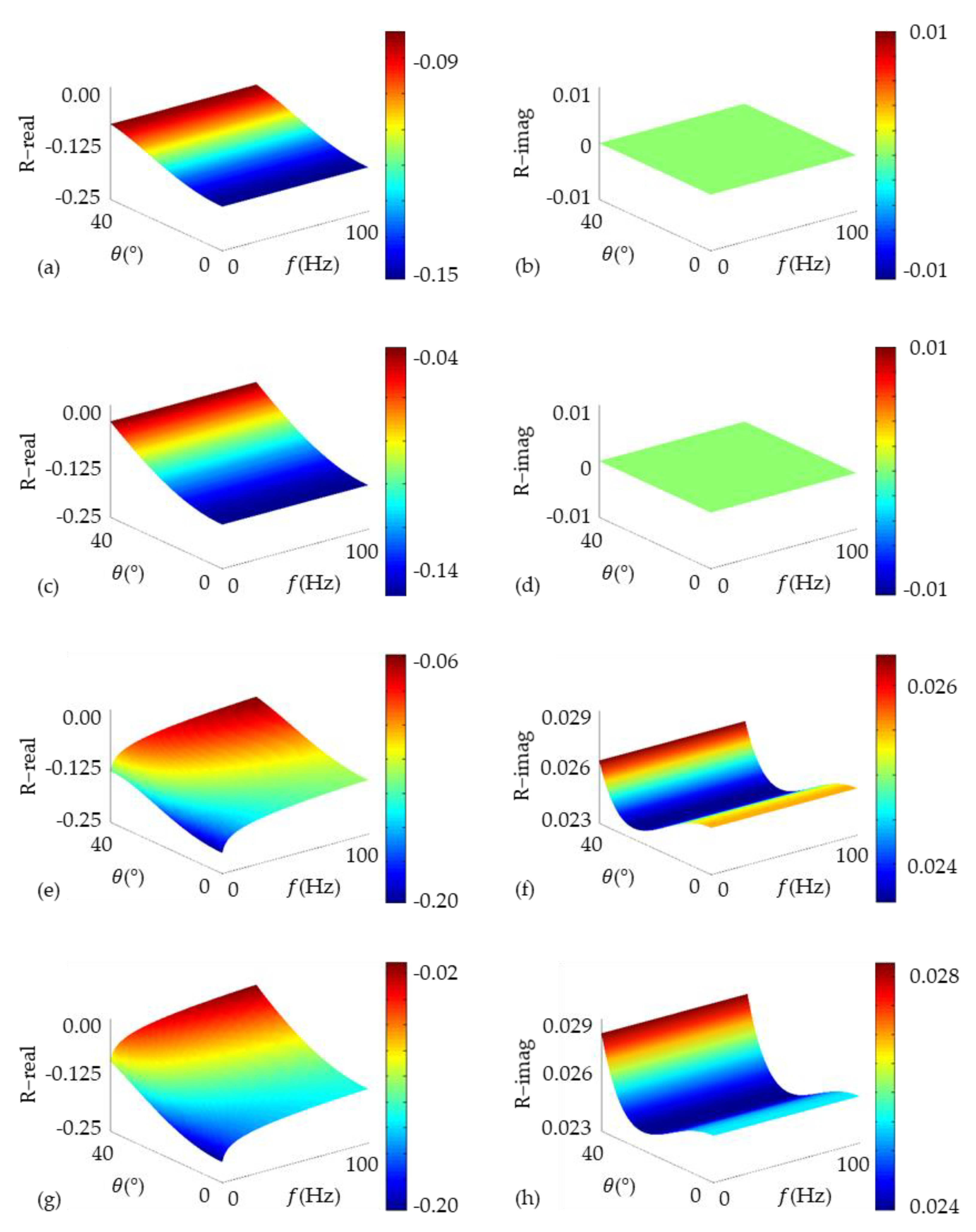
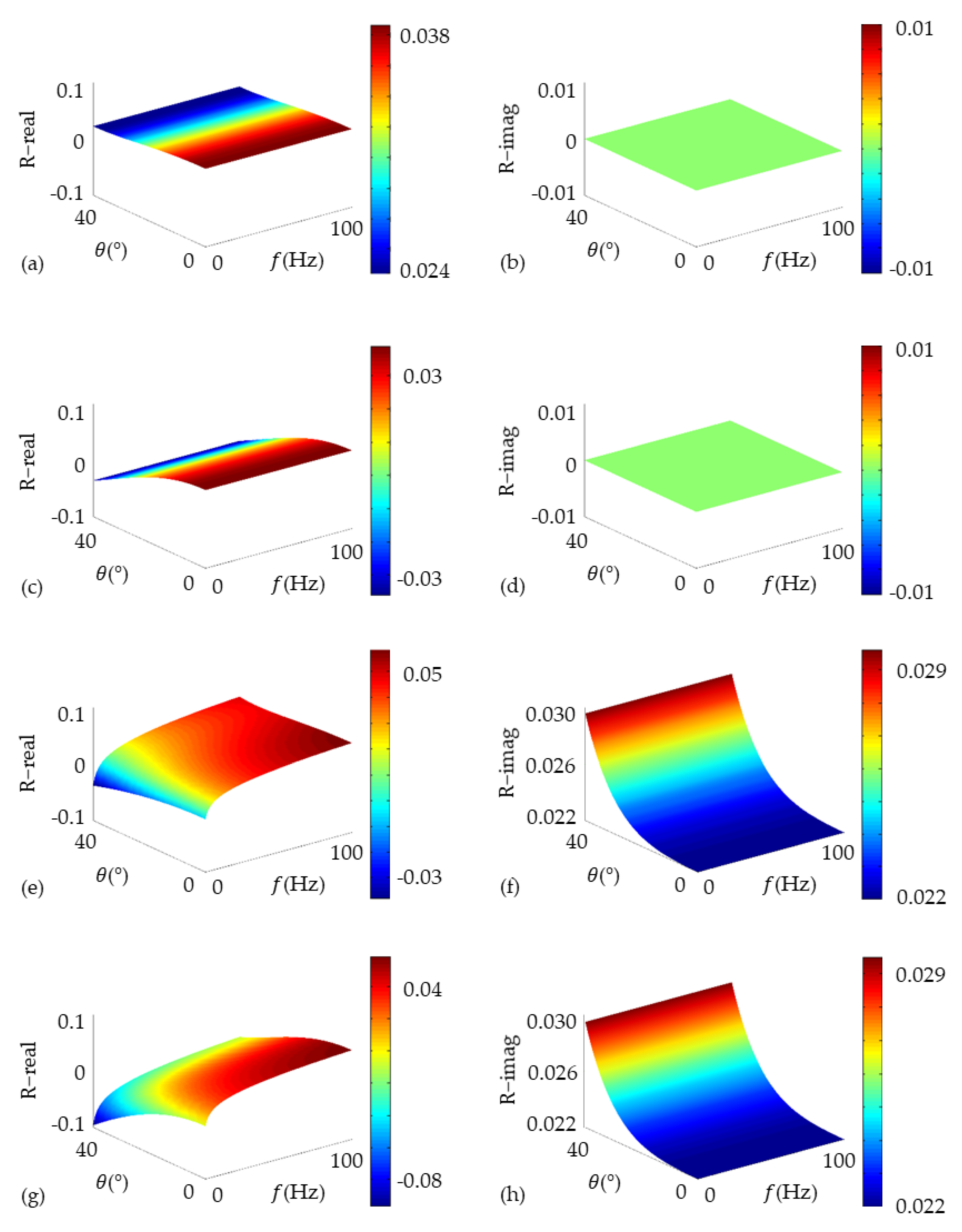
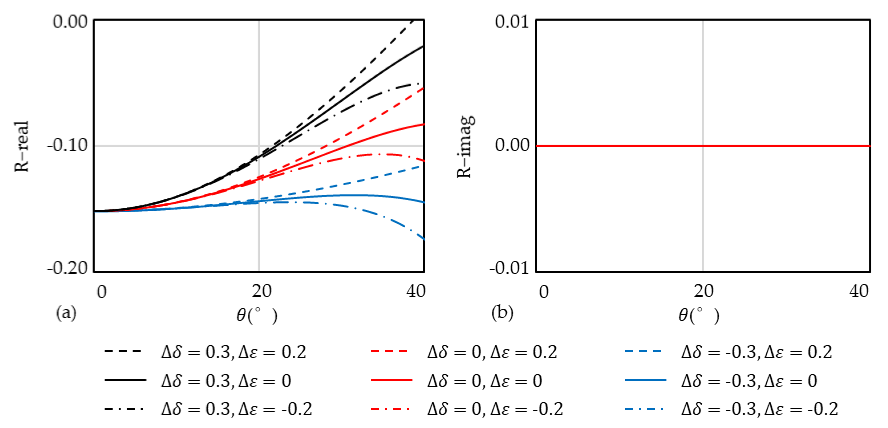
3.1. Characteristics of Reflection Coefficients for Q-VTI Model

To analyze the characteristics of reflection coefficients, we compute the reflection coefficients around the solution point of the interface of two models using the derived reflection coefficient equation. Parameters of two models are shown in Table 1 and Table 2 separately. For Model 1, we take the mud shale as the upper layer and oil shale as the lower layer, and for Model 2, we take the mud shale as the upper layer but calcareous sandstone as the lower layer. The properties of background and perturbation are the average value and the difference value of two layers, respectively. The elastic and anisotropic parameters of two models come from the compiled table of Thomsen [25] about the measured anisotropy in sedimentary rocks.
Figure 2 and Figure 3 show the variation of reflection coefficients with the incident angle θ and frequency f for Model 1 and 2, respectively. We consider four cases of (1) elastic isotropy, (2) elastic anisotropy, (3) attenuated isotropy, and (4) attenuated anisotropy to compute the reflection coefficients using the derived reflection coefficient equation. The results show in sub-Figure (a,b), (c,d), (e,f) and (g,h), respectively and the value of colors represent in corresponding colorbars, where sub-Figure (a,c,e,f) and (b,d,f,h) exhibit the real part and the imaginary part of reflection coefficients separately. We stress that all parameters of the same properties on the vertical axis have the same scale so that the different degree of various influence can be observed directly.
In the case of elastic isotropic assumption, the derived reflection coefficient becomes the linearized P-P reflection coefficient given by Aki and Richards [16]. Therefore, the reflection coefficients are real numbers and controlled only by P-wave velocity α , S-wave velocity β and density ρ . In Figure 2a, we observe the real parts of reflection coefficients increase with the incident angle but frequency-independent. It exhibits the fourth AVO type in the case of the interface separating the mud shale and oil shale model. In Figure 2b, we observe that the imaginary parts of reflection coefficients are equal to zero.
The derived reflection coefficient is exactly the same as the reflection coefficient proposed by Rüger [30,31] when we only take the effect of anisotropy into consideration. The reflection coefficients are frequency-independent, as shown in Figure 2c, and the imaginary parts are also zero, as shown in Figure 2d. We conclude that the anisotropic parameters ε , δ just affect the value of reflection coefficients, however, the AVO type is the same as Figure 2a.
It shows slightly difference in the case of attenuated isotropic assumption. The reflection coefficients become complex numbers, and vary with both incident angle and frequency, as shown in Figure 2e. We emphasize that the AVO type has not been changed by the attenuation parameters Q p 1 , Q s 1 . In Figure 2f, we observe the imaginary part of reflection coefficients vary with incident angle but frequency-independent.
Figure 2g,h show the characteristics of the complex reflection coefficients in the case of attenuated anisotropic assumption, which are the similar to the results of reflection coefficients for the attenuated isotropic assumption. We observe the Thomsen-style attenuation-anisotropic parameters ε Q , δ Q have litter effect in larger incident angles and higher frequency on the reflection coefficients.
Then, we compute the reflection coefficients around the solution point of the interface separating the mud shale and calcareous sandstone. The same characteristics appear in this model, as shown in Figure 3. We observe the reflection coefficients decrease with the incident angle but frequency-independent in Figure 3a. It exhibits the second AVO type in the case of model 2 due to P-wave velocity α , S-wave velocity β and density ρ . The anisotropic parameters ε , δ also only affect the value of reflection coefficients and the AVO type doesn’t change, as shown in Figure 3c. Figure 3e–h show that the reflection coefficients are complex numbers and the real parts vary with frequency caused by the attenuation. However, the Thomsen-style attenuation-anisotropic parameters ε Q , δ Q contribute much smaller to the reflection coefficient than Q p 1 and Q s 1 because they exist in the terms of high order.
In the following, we focus on the effect of the crucial parameters of anisotropy ε , δ and attenuation Q p 1 , Q s 1 . We proceed to the analysis of how perturbations in anisotropic parameters and attenuation factors affect reflection coefficients. The P-wave velocity α , S-wave velocity β and density ρ are set up as the same as the model 1 (Table 1), and nine groups of perturbations in anisotropic Δ δ , Δ ε and six groups of perturbations in attenuation Δ Q p 1 , Δ Q s 1 , as shown in Table 3 and Table 4. Using the derived reflection coefficient equation, we obtain the reflection coefficients variation with incident angle and frequency in the case of different perturbations.
We first consider the effect of perturbations in anisotropy ∆δ and ∆ε on the reflection coefficients, as shown in Figure 4. For this case, the derived linearized reflection coefficient is equal to the reflection coefficient proposed by Rüger [30,31] because the attenuation parameters are neglected. In Figure 4a we observe the reflection coefficients are frequency-independent, and in Figure 4b we observe the imaginary part of reflection coefficients are equal to zero. In Figure 4a, the intercept of reflection coefficients is a constant, and equals to the result computed for the isotropic model (the red solid line). By comparing three sets of the same type of lines (dashed lines, solid lines and doted dashed lines), respectively, we observe the gradients of curves vary with ∆δ. For example, the gradients of blue dashed line, red dashed line and black dashed line increase with ∆δ when ∆ε is equal to a constant 0.2, but the curvature of them are the same. In the meanwhile, we observe the curvatures vary with ∆ε by comparing three sets of same color of lines (black lines, red lines, and blue lines), respectively. For example, the curvatures of black doted dashed line, black solid line and black dashed line increase with ∆ε when ∆δ is equal to a constant 0.3, but the gradient of them is a constant. It appears the same characteristics in the rest groups.
Next, we analyze the effect of perturbations in P- and S-wave attenuation factors Δ Q p 1 , Δ Q s 1 on the reflection coefficients, as shown in Figure 5. For this case, we neglect the parameters of anisotropy and attenuation anisotropy. Figure 5a–f show the real and imaginary parts of reflection coefficients computed using six combinations of attenuation parameters presented in legend in three case of frequency: (1) 5 Hz, (2) 25 Hz and (3) 65 Hz. We mention that the reference frequency is 25 Hz. In Figure 5, we observe that the reflection coefficients are complex numbers, and the real part is frequency-dependent; however, the imaginary part is frequency-independent.
Figure 5a shows the effect of Δ Q p 1 , Δ Q s 1 on the real part of reflection coefficients when the frequency is equal to 5 Hz. The red solid line represents the result computed for the elastic isotropic model because the attenuation parameters are equal to zero. By comparing the solid line of red, black and blue, the intercept, gradient and curvature of them all decrease with the inverse quality factor of P-wave Δ Q p 1 . Three blue lines illustrate the inverse quality factor of S-wave Δ Q s 1 only affects the gradient of the real parts and increases it. Figure 5c shows the real part of reflection coefficients are equal to the result of elastic isotropic assumption in 25 Hz since the natural logarithm of frequency term becomes zero when the frequency we took is equal to reference frequency. Figure 5e shows the effect of Δ Q p 1 , Δ Q s 1 on the real part of reflection coefficients when the frequency is equal to 65 Hz. By comparing the solid line of red, black and blue, the intercept, gradient and curvature of them all increase with the inverse quality factor of P-wave Δ Q p 1 . Three blue lines illustrate the inverse quality factor of S-wave Δ Q s 1 only affects the gradient of the real parts but decreases it.
We conclude the imaginary part of reflection coefficients are frequency- independent, as shown in Figure 5b,d,e. By comparing the solid line of red, black and blue, the intercept, gradient and curvature of the imaginary parts all increase with the inverse quality factor of P-wave Δ Q p 1 . However, the gradient of the imaginary part decreases with the inverse quality factor of S-wave Δ Q s 1 which is illustrated by three blue lines.

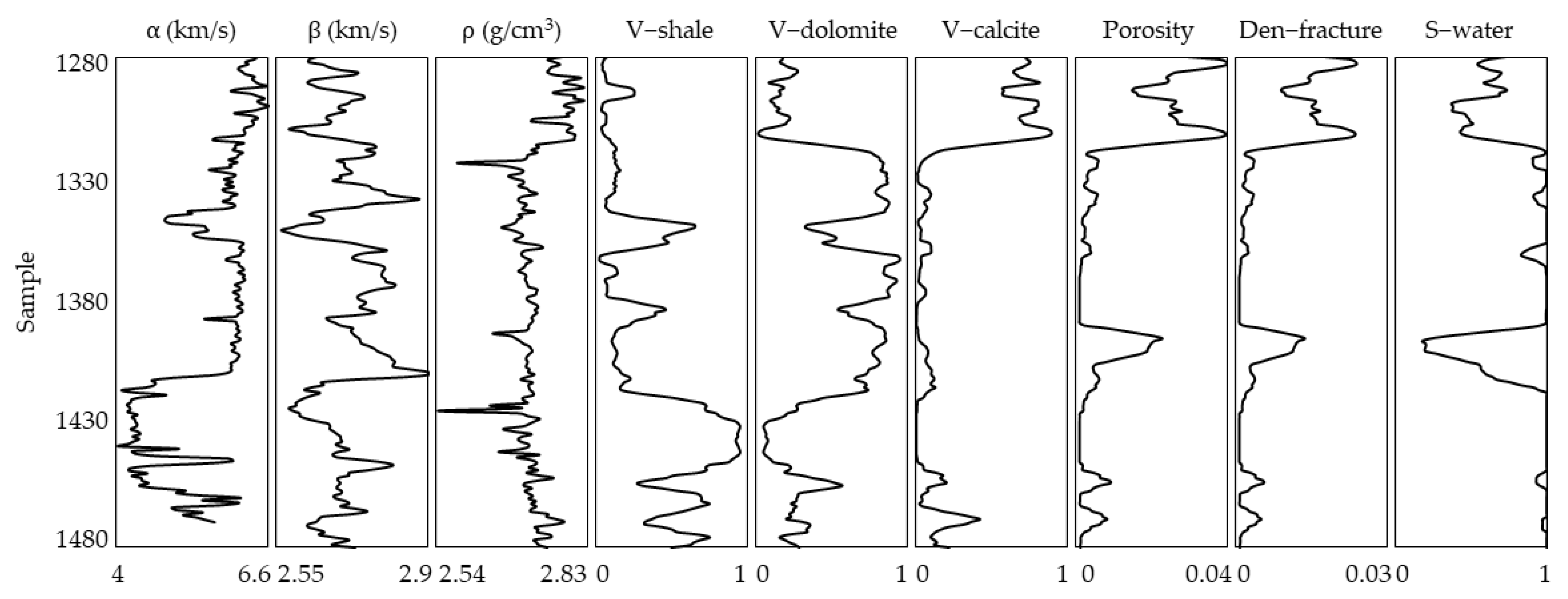
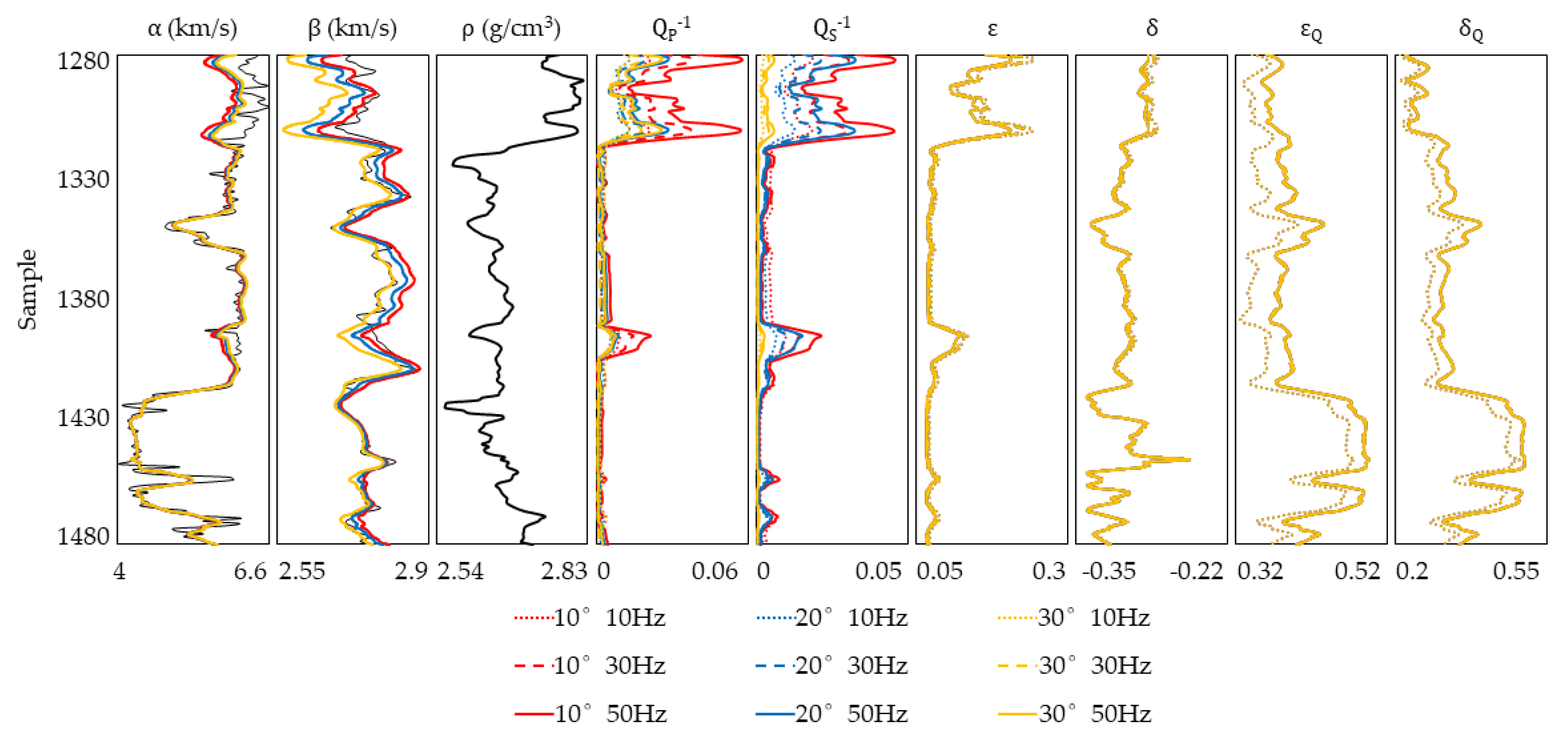
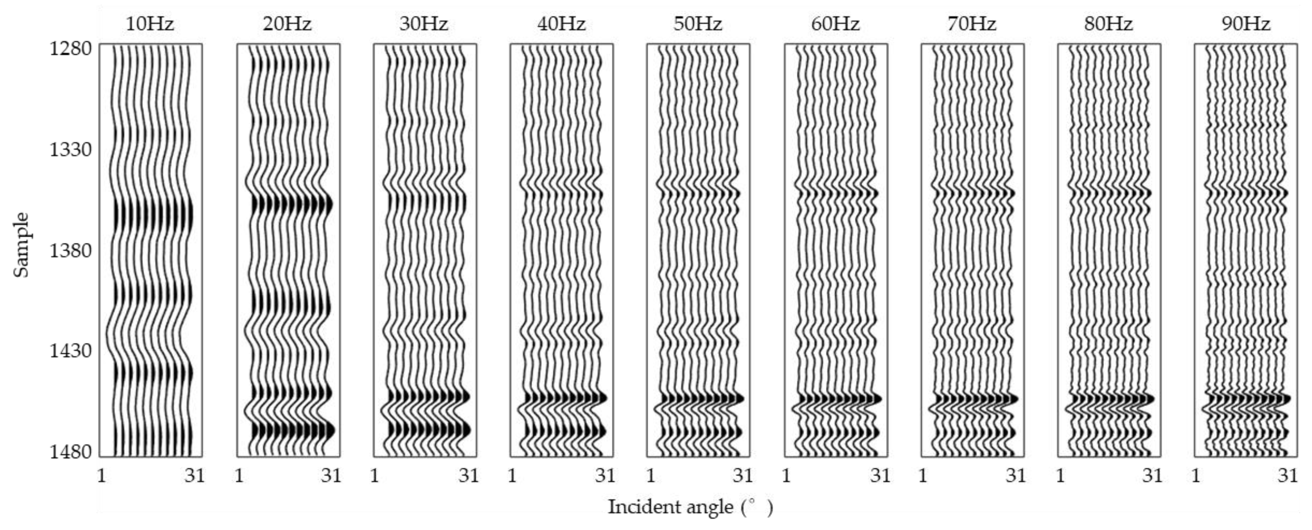
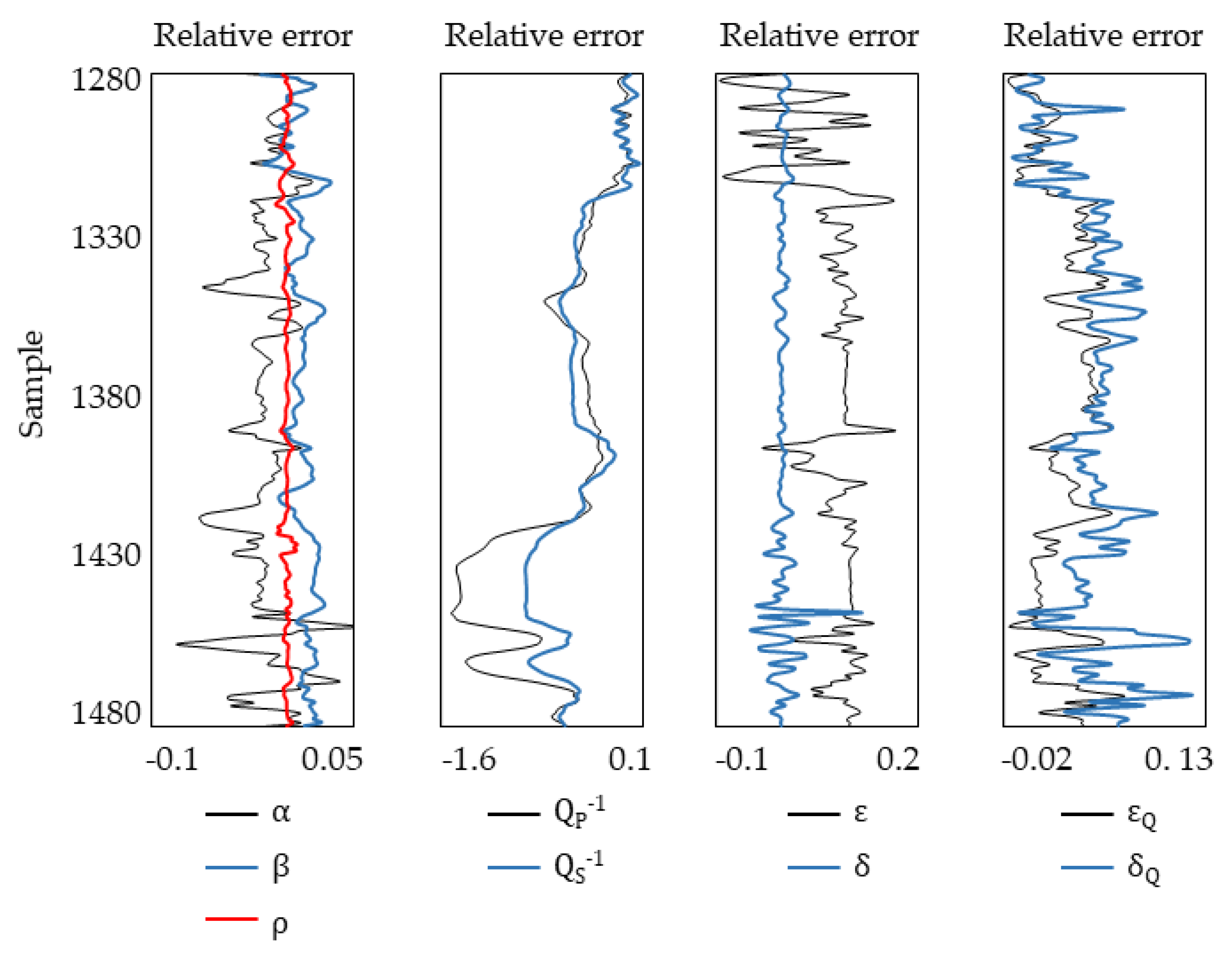
3.2. Inversion Test for Q-VTI Model

We use the synthetic seismic data to verify the feasibility of the proposed equation for inversion. At first, we choose a well logging data to build a fractured model which is shown in Figure 6. We find that the places with high calcite content developing pores and fractures bearing fluids, and there is no good correspondence of the basis elastic parameters P- and S-wave velocity with it.
Then, we calculate the complex stiffness matrix using Chapman model [4,5,6] and further obtain the P- and S-wave velocity, density, inverse quality factors, anisotropic parameters and Thomsen-style attenuated anisotropic parameters. As is shown in Figure 7, we acquire these new parameters which is vary with different frequency and incident angle. The P- and S-wave velocities exhibit in this figure are their real parts, and the P- and S-wave velocity we estimated match well with the measured value except some differences in the place of pore, fracture and fluid anomaly. Significantly, the inverse quality factors of P- and S-wave show obvious differences in both frequency and incident angle especially in pore, fracture and fluid anomaly. These small differences are apparent because they are orders of magnitude smaller. They represent the ratio of the imaginary and real parts of P- and S-wave velocity, which is reflect the attenuation characteristics of P- and S-wave. What’s more, the trends of Q p 1 , Q s 1 and ε are more consistent with that of porosity, fracture density and fluid saturation than α and β .
Next, we generate synthetic seismic data in small incident angles utilizing Ricker wavelets with different frequencies, as is shown in Figure 8. We add Gaussian random noise into the synthetic seismic data to generate noisy seismic data of signal-to-noise ratio being 5. The result is shown in Figure 9 and used as the observed seismic data for inversion through the Equation (12).
Figure 10 plots comparisons between true values of model and inversion results of each parameter. We take the average value estimated by the Chapman model as the true value for comparison, and calculate the relative error of each inverted parameter, as shown in Figure 11. We observe a close match between inversion results and true values given data with a moderate noise.

4. Result and Discussion

It is possible to obtain relatively simple approximations for the PP-wave reflection coefficient of the linear constant Q -VTI model under the assumption of weak anisotropy and low-loss attenuation of velocities. One of the advantages is the Q-VTI model considers frequency dispersion and anisotropy of velocities at the same time. Another advantage is the equation decouple the inverse quality factors of P- and S-wave and the Thomson-style attenuation anisotropic factors from the complex velocities and Thomson anisotropy parameters. Based on the derived reflection coefficient, we analyze some characteristics of reflection coefficients in the case of different reservoirs and groups of parameters.
The type of AVO is determined by the differences in P-wave velocity, S-wave velocity and density across the interface. Both the anisotropic parameters and the attenuation parameters only change the value of the reflection coefficient; however, they don’t affect the type of AVO. The perturbations of anisotropy Δ δ and Δ ε contribute to the gradient and the curvature. The perturbations in attenuated anisotropy Δ δ Q and Δ ε Q also contribute to the gradient and the curvature, but the contribution is much smaller than that of Δ δ and Δ ε . The attenuation factor of P-wave Δ Q p 1 affects the intercept, gradient and curvature at the same time, however, the attenuation factor of S-wave Δ Q s 1 only affects the gradient.
The reflection coefficients become complex numbers when we consider the effect of the attenuation, in which the real part represents the amplitude and the imaginary part represents the phase. The real parts of reflection coefficients vary with the frequency caused by the attenuation terms, however, the imaginary parts are frequency-independent. The real part of reflection coefficient is inversely proportional to Δ Q p 1 but proportional to Δ Q s 1 because the natural logarithm of frequency term is negative when the frequency is less than the reference frequency. In the same way, the real part of reflection coefficient is proportional to Δ Q p 1 but inversely proportional to Δ Q s 1 because the natural logarithm of frequency term is positive when the frequency is greater than the reference frequency. In particular, the reflection coefficient to be equivalent to the elastic cases because the natural logarithm of frequency term becomes zero when the frequency we took is equal to the reference frequency.
The contribution of the attenuation anisotropic term that the high order to the reflection coefficient is very small compared with other properties. In the meanwhile, the value of third term which affects the reflection coefficient at a large incident angle is much smaller than the first two terms when the P-wave incident at a small angle.
We observe that the relative error of inverse quality factors seems to be large, which is still caused by their relatively small order of magnitude than other parameters, but the trend of their inversion results is completely consistent with the true values. Thus, we still regard the inversion test shows a well result to verify the feasibility of the proposed equation. In addition, the attenuated and anisotropic parameters are not only the better indicators of pores, fractures and fluids than the P- and S-wave velocity, but also enable us to avoid further inversion of physical parameters such as porosity, fracture density and fluid saturation.

5. Summary and Conclusions

Under the assumption of low-loss attenuation and weak anisotropy of velocities, we derive the linearized approximate frequency-dependent reflection coefficient based on the linear constant Q-VTI model. We observe that the reflection coefficient is related to the parameters of anisotropy and attenuation simultaneously, and varies with both the incident angle and frequency. It appears that the analysis of the AVOF characteristics may guide us to identify the characteristics of anisotropy and attenuation in the real working area, and we can take full advantage of the seismic data of different incident angles and frequencies to predict the fluid-filled pores and fractures in the reservoirs using our derived reflection coefficient equation.
Moreover, the attenuated anisotropic medium is more suitable for modeling how seismic wave propagates in underground layers than that proposed under the assumption of elastic isotropic or anisotropic medium. Focusing on the attenuated anisotropic medium, we consider the effects of Thomsen parameters that are related to anisotropy caused by fractures and the attenuation factors that are sensitive to attenuation caused by intrinsic attenuation and the fluid-filled in pores and fractures on the reflection coefficient, which may provide more useful information for detecting fractures and fluids using the observed seismic data. We conclude that we present a valuable expression of reflection coefficient, which can be employed for the analysis of seismic wave response modeling for different types of reservoirs, and the derived reflection coefficient can also guide the inversion for the properties that are related to fractures and fluids using frequency components of seismic amplitudes.

Author Contributions

Conceptualization, Y.Y. and X.Y.; methodology, Y.Y. and G.G.; software, Y.Y. and G.G.; validation, Y.Y., X.Y., G.G., D.C. and B.Z.; formal analysis, Y.Y.; investigation, Y.Y.; resources, D.C.; data curation, D.C.; writing—original draft preparation, Y.Y.; writing—review and editing, B.Z.; visualization, Y.Y.; supervision, X.Y.; project administration, X.Y.; funding acquisition, X.Y. All authors have read and agreed to the published version of the manuscript.

Funding

This research was funded by the National Natural Science Foundation of China (42030103, 42004092).

Acknowledgments

The authors would like to acknowledge the many current and past researchers who have contributed to the foundational work for this study. We also thank the anonymous reviewers and editors for their constructive suggestions.

Conflicts of Interest

The authors declare no conflict of interest.

Appendix A

The complex stiffness matrix of the Q-VTI medium can be re-expressed as the sum of the anisotropic perturbation and the stiffness matrix of a homogeneous isotropic background based on the perturbation theory.
c ˜ Q V T I = [ c ˜ 11 c ˜ 11 2 c ˜ 66 c ˜ 13 0 0 0 c ˜ 11 2 c ˜ 66 c ˜ 11 c ˜ 13 0 0 0 c ˜ 13 c ˜ 23 c ˜ 33 0 0 0 0 0 0 c ˜ 55 0 0 0 0 0 0 c ˜ 55 0 0 0 0 0 0 c ˜ 66 ] = [ c ˜ 33 0 c ˜ 33 0 2 c ˜ 55 0 c ˜ 33 0 2 c ˜ 55 0 0 0 0 c ˜ 33 0 2 c ˜ 55 0 c ˜ 33 0 c ˜ 33 0 2 c ˜ 55 0 0 0 0 c ˜ 33 0 2 c ˜ 55 0 c ˜ 33 0 2 c ˜ 55 0 c ˜ 33 0 0 0 0 0 0 0 c ˜ 55 0 0 0 0 0 0 0 c ˜ 55 0 0 0 0 0 0 0 c ˜ 55 0 ] + [ Δ c ˜ 33 Δ c ˜ 33 2 Δ c ˜ 55 Δ c ˜ 33 2 Δ c ˜ 55 0 0 0 Δ c ˜ 33 2 Δ c ˜ 55 Δ c ˜ 33 Δ c ˜ 33 2 Δ c ˜ 55 0 0 0 Δ c ˜ 33 2 Δ c ˜ 55 Δ c ˜ 33 2 Δ c ˜ 55 Δ c ˜ 33 0 0 0 0 0 0 Δ c ˜ 55 0 0 0 0 0 0 Δ c ˜ 55 0 0 0 0 0 0 Δ c ˜ 55 ] + [ c ˜ 11 c ˜ 33 c ˜ 12 c ˜ 33 + 2 c ˜ 55 c ˜ 13 c ˜ 33 + 2 c ˜ 55 0 0 0 c ˜ 12 c ˜ 33 + 2 c ˜ 55 c ˜ 11 c ˜ 33 c ˜ 13 c ˜ 33 + 2 c ˜ 55 0 0 0 c ˜ 13 c ˜ 33 + 2 c ˜ 55 c ˜ 13 c ˜ 33 + 2 c ˜ 55 0 0 0 0 0 0 0 0 0 0 0 0 0 0 0 0 0 0 0 0 0 c ˜ 66 c ˜ 55 ]
where, the stiffness coefficients in the square brackets on the right-hand side represent isotropic attenuated background, isotropic attenuated perturbations and anisotropic attenuated perturbations, respectively.
The polarization vectors and slowness vectors corresponding the incident and reflected waves are given by,
t = [ sin θ cos φ , sin θ sin φ , cos θ ] t = [ sin θ cos φ , sin θ sin φ , cos θ ] p = ( 1 / v ˜ ) [ sin θ cos φ , sin θ sin φ , cos θ ] p = ( 1 / v ˜ ) [ sin θ cos φ , sin θ sin φ , cos θ ]

References

  1. Thomsen, L. Elastic anisotropy due to aligned cracks in porous rock. Geophys. Prospect. 1995, 43, 805–829. [Google Scholar] [CrossRef]
  2. Carcione, J.M. Constitutive model and wave equations for linear, viscoelastic, anisotropic media. Geophysics 1995, 60, 537–548. [Google Scholar] [CrossRef]
  3. Carcione, J.M. Wave Fields in Real Media: Wave Propagation in Anisotropic, Anelastic, Porous and Electromagnetic Media, 2nd ed.; Elsevier: Amsterdam, The Netherlands, 2007. [Google Scholar]
  4. Chapman, M. Frequency-dependent anisotropy due to meso-scale fractures in the presence of equate porosity. Geophys. Prospect. 2003, 51, 369–379. [Google Scholar] [CrossRef] [Green Version]
  5. Chapman, M.; Liu, E.; Li, X. The influence of fluid-sensitive dispersion and attenuation on AVO analysis. Geophys. J. Int. 2006, 167, 89–105. [Google Scholar] [CrossRef] [Green Version]
  6. Chapman, M. Modeling the effect of multiple sets of mesoscale fractures in porous rock on frequency-dependent anisotropy. Geophysics 2009, 74, D97–D103. [Google Scholar] [CrossRef] [Green Version]
  7. Ba, J.; Cao, H.; Yao, F.; Nie, J.; Yang, H. Double-porosity rock model and squirt flow in the laboratory frequency band. Appl. Geophys. 2008, 5, 261–276. [Google Scholar] [CrossRef]
  8. Guo, J.; Shuai, D.; Wei, J.; Ding, P.; Gurevich, B. P-wave dispersion and attenuation due to scattering by aligned fluid saturated fractures with finite thickness: Theory and experiment. Geophys. J. Int. 2018, 215, 2114–2133. [Google Scholar] [CrossRef]
  9. Guo, J.; Gurevich, B.; Shuai, D. Frequency-dependent P-wave anisotropy due to scattering in rocks with aligned fractures. Geophysics 2020, 85, MR97–MR105. [Google Scholar] [CrossRef]
  10. Thanh, H.V.; Sugai, Y.; Nguele, R.; Sasaki, K. A New Petrophysical Modeling Workflow for Fractured Granite Basement Reservoir in Cuu Long Basin, Offshore Vietnam. In Proceedings of the 81st EAGE conference and exhibition, London, UK, 3–6 June 2019; pp. 1–5. [Google Scholar] [CrossRef]
  11. Thanh, H.V.; Sugai, Y.; Nguele, R.; Sasaki, K. Integrated workflow in 3D geological model construction for evaluation of CO2 storage capacity of a fractured basement reservoir in Cuu Long Basin, Vietnam- Sciencedirect. Int. J. Greenh. Gas Control 2019, 90, 102826. [Google Scholar] [CrossRef]
  12. Schoenberg, M. Elastic wave behavior across linear slip interfaces. J. Acoust. Soc. Am. 1980, 68, 1516–1521. [Google Scholar] [CrossRef] [Green Version]
  13. Hudson, J.A. Wave speeds and attenuation of elastic waves in material containing cracks. Geophys. J. Int. 1981, 64, 133–150. [Google Scholar] [CrossRef]
  14. Gurevich, B. Elastic properties of saturated porous rocks with aligned fractures. J. Appl. Geophys. 2003, 54, 203–218. [Google Scholar] [CrossRef]
  15. Chapman, M.; Maultzsch, M.; Liu, E.; Li, X. The effect of fluid saturation in an anisotropic multi-scale equant porosity model. J. Appl. Geophys. 2003, 54, 191–202. [Google Scholar] [CrossRef]
  16. Aki, K.; Richards, P.G. Quantitative Seismology: Theory and Methods; W.H. Freeman: San Francisco, CA, USA, 1980; p. 932. [Google Scholar]
  17. Shaw, R.K.; Sen, M.K. Use of AVOA data to estimate fluid indicator in a vertically fractured medium. Geophysics 2006, 71, C15–C24. [Google Scholar] [CrossRef]
  18. Zong, Z.; Yin, X.; Wu, G. Complex seismic amplitude inversion for P-wave and S-wave quality factors. Geophys. J. Int. 2015, 202, 564–577. [Google Scholar] [CrossRef]
  19. Moradi, S.; Innanen, K.A. Born scattering and inversion sensitivities in viscoelastic transversely isotropic media. Geophys. J. Int. 2017, 211, 1177–1188. [Google Scholar] [CrossRef]
  20. Moradi, S. Scattering of Seismic Waves from Arbitrary Viscoelastic-Isotropic and Anisotropic Structures with Applications to Data Modelling, FWI Sensitivities and Linearized AVO-AVAz Analysis. Ph.D. Thesis, University of Calgary, Calgary, AB, Canada, 2017. [Google Scholar]
  21. Chen, H.; Innanen, K.A.; Chen, T. Estimating P- and S-wave inverse quality factors from observed seismic data using an attenuative elastic impedance. Geophysics 2018, 83, R173–R187. [Google Scholar] [CrossRef]
  22. Chen, H.; Li, J.; Innanen, K.A. Inversion of differences in frequency components of azimuthal seismic data for indicators of oil-bearing fractured reservoirs based on an attenuative cracked model. Geophysics 2020, 85, 1MJ-Z13. [Google Scholar] [CrossRef]
  23. Pan, X.; Zhang, G.; Cui, Y. Matrix-fluid-fracture decoupled-based elastic impedance variation with angle and azimuth inversion for fluid modulus and fracture weaknesses. J. Pet. Sci. Eng. 2020, 189, 106974. [Google Scholar] [CrossRef]
  24. Kjartansson, E. Constant Q-wave propagation and attenuation. J. Geophys. Res. Atmos. 1979, 84, 4737–4748. [Google Scholar] [CrossRef] [Green Version]
  25. Thomsen, L. Weak elastic anisotropy. Geophysics 1986, 51, 1954–1966. [Google Scholar] [CrossRef]
  26. Thomsen, L. Reflection seismology over azimuthally anisotropic media. Geophysics 1988, 53, 304–313. [Google Scholar] [CrossRef]
  27. Zhu, Y.; Tsvankin, I. Plane-wave propagation in attenuative transversely isotropic media. Geophysics 2006, 71, T17–T30. [Google Scholar] [CrossRef] [Green Version]
  28. Zhu, Y.; Tsvankin, I.; Dewangan, P.; Wijk, K.V. Physical modeling and analysis of P-wave attenuation anisotropy in transversely isotropic media. Geophysics 2007, 72, D1–D7. [Google Scholar] [CrossRef]
  29. Shaw, R.K.; Sen, M.K. Born integral, stationary phase and linearized reflection coefficients in weak anisotropic media. Geophys. J. Int. 2004, 158, 225–238. [Google Scholar] [CrossRef] [Green Version]
  30. Rüger, A. Reflection Coefficients and Azimuthal AVO Analysis in Anisotropic Media. Ph.D. Thesis, Colorado School of Mines, Denver, CO, USA, 1996. [Google Scholar]
  31. Rüger, A. Variation of P-wave reflectivity with offset and azimuth in anisotropic media. Geophysics 1998, 63, 935–947. [Google Scholar] [CrossRef]
  32. Shuey, R.T. A simplification of the Zoeppritz equations. Geophysics 1985, 50, 609–614. [Google Scholar] [CrossRef]
Figure 1. Schematic of seismic wave propagate in an attenuation anisotropy medium based on the perturbation theory. It is characterized by three elastic parameters P-wave velocity α , S-wave velocity β and density ρ ; two viscoelastic parameters P-wave quality factor Q P and S-wave quality factor Q S ; three anisotropic Thomsen parameters ε ,   γ ,   δ and corresponding attenuation Thomsen parameters ε Q ,   γ Q ,   δ Q . Note that the subscript ‘0′ stands for the properties of background (reference medium) and the mark ‘ Δ ’ stands for the properties of small perturbation.
Energies 14 08506 g001
Figure 2. The variation of reflection coefficient with the incident angle θ and frequency f for model 1. (a,b), (c,d), (e,f) and (g,h) show the real part and imaginary part of reflection coefficients in four cases of assumption: (1) elastic isotropy, (2) elastic anisotropy, (3) attenuated isotropy, and (4) attenuated anisotropy separately. Different reflection coefficient values represent in corresponding colorbars.
Energies 14 08506 g002
Figure 3. The variation of reflection coefficient with the incident angle θ and frequency f for model 2. (a,b), (c,d), (e,f) and (g,h) show the real part and imaginary part of reflection coefficients in four cases of assumption: (1) elastic isotropy, (2) elastic anisotropy, (3) attenuated isotropy, and (4) attenuated anisotropy separately. Different reflection coefficient values represent in corresponding colorbars.
Energies 14 08506 g003
Figure 4. The effect of anisotropic parameters Δ ε and Δ δ on the reflection coefficients. At this point, the reflection coefficients are real numbers and frequency-independent. (a) shows the real part of it in nine combinations of anisotropy parameters, and (b) shows the imaginary part equal to zero.
Energies 14 08506 g004
Figure 5. The effect of attenuation parameters Δ Q p 1 and Δ Q s 1 on the reflection coefficients. At this point, the reflection coefficients are complex numbers and frequency-dependent. (af) show the real part and imaginary part of reflection coefficients in three cases of 5 Hz, 25 Hz and 65 Hz separately. Different lines exhibit the results of six combinations of attenuation parameters. The reference frequency is set to 25 Hz.
Energies 14 08506 g005
Figure 6. The well logging data of a fractured model which is ready to calculate the attenuated and anisotropic parameters.
Energies 14 08506 g006
Figure 7. The estimated results of the attenuated and anisotropic parameters using Chapman model in different frequency and incident angle. The black lines are the measured values from well-logging.
Energies 14 08506 g007
Figure 8. The synthetic seismic data for a set of frequency in small incident angles.
Energies 14 08506 g008
Figure 9. The synthetic seismic data which added Gaussian random noise with S/N of 5. These results will be used as the observed seismic data for inversion. The lower frequency data affected more by noises.
Energies 14 08506 g009
Figure 10. Comparison of the inverted results and true values of the P- and S-wave velocity, density, inverse quality factors, anisotropic parameters and Thomsen-style attenuated anisotropic parameters.
Energies 14 08506 g010
Figure 11. The relative errors between inverted result and model value of each parameter.
Energies 14 08506 g011
Table 1. The parameters of attenuated anisotropic model 1.
Layer α
(km/s)
β
(km/s)
ρ
(g/cm3)
ε δ Q P 1 Q S 1 ε Q δ Q
Mud-shale5.0732.9982.680.0100.0120.0010.0010.0010.001
Oil-shale4.2312.5392.370.2000.1000.2050.1180.0460.025
Table 2. The parameters of attenuated anisotropic model 2.
Layer α
(km/s)
β
(km/s)
ρ
(g/cm3)
ε δ Q P 1 Q S 1 ε Q δ Q
Mud-shale5.0732.9982.680.0100.0120.0010.0010.0010.001
Calcareous Sandstone5.4603.2192.690.000−0.2640.1770.056−0.0250.050
Table 3. The effect of elastic anisotropic perturbation on the reflection coefficient.
Anisotropic Perturbation123
Δ δ 0.30−0.3
Δ ε 0.2, 0, −0.20.2, 0, −0.20.2, 0, −0.2
Table 4. The effect of attenuated isotropic perturbation on the reflection coefficient.
Attenuated Perturbation123
Δ Q P 1 00.020.2
Δ Q S 1 00, 0.0120, 0.012, 0.12
Publisher’s Note: MDPI stays neutral with regard to jurisdictional claims in published maps and institutional affiliations.

