
Exploring of the Incompatibility of Marine Residual Fuel: A Case Study Using Machine Learning Methods


1
Department of Oil and Gas Transport and Storage, Saint Petersburg Mining University, 199106 Saint Petersburg, Russia
2
Department of Automation of Technological Processes and Production, Saint Petersburg Mining University, 199106 Saint Petersburg, Russia
3
Department of Petroleum Engineering, Saint Petersburg Mining University, 199106 Saint Petersburg, Russia
4
Faculty of Science and Technology, University of Stavanger, 4036 Stavanger, Norway
*
Author to whom correspondence should be addressed.
Energies 2021, 14(24), 8422; https://doi.org/10.3390/en14248422
Submission received: 31 October 2021
/
Revised: 29 November 2021
/
Accepted: 9 December 2021
/
Published: 14 December 2021
(This article belongs to the Section H1: Petroleum Engineering)
Abstract
:Providing quality fuel to ships with reduced SOx content is a priority task. Marine residual fuels are one of the main sources of atmospheric pollution during the operation of ships and sea tankers. Hence, the International Maritime Organization (IMO) has established strict regulations for the sulfur content of marine fuels. One of the possible technological solutions allowing for adherence to the sulfur content limits is use of mixed fuels. However, it carries with it risks of ingredient incompatibilities. This article explores a new approach to the study of active sedimentation of residual and mixed fuels. An assessment of the sedimentation process during mixing, storage, and transportation of marine fuels is made based on estimation three-dimensional diagrams developed by the authors. In an effort to find the optimal solution, studies have been carried out to determine the influence of marine residual fuel compositions on sediment formation via machine learning algorithms. Thus, a model which can be used to predict incompatibilities in fuel compositions as well as sedimentation processes is proposed. The model can be used to determine the sediment content of mixed marine residual fuels with the desired sulfur concentration.
1. Introduction
Greenhouse gas emissions from ships, especially sulfur oxides (SOx), have serious impacts on human health, the marine environment, and natural resources. Dozens of countries, including China and the EU, have already announced their readiness to achieve carbon neutrality on their territory by 2050–2060, i.e., to reduce to zero the difference between greenhouse gas emissions and their absorption by taking into account the capabilities of the region’s ecosystem. The EU was one of the first to propose a transition to a carbon neutral economy by 2050 within the framework of the European Green Deal [1]. To achieve the goal of decarbonization and sustainable development of the fuel and energy complex in Russia, unprecedented legislative measures have been taken [2,3,4,5,6] by aiming at tax benefits for domestic majors, and this stimulates research projects aimed at reducing emissions of harmful gases [7,8,9,10]. The EU has already launched CO2 emissions quotas, and the EU Emissions Trading System has begun to operate. Transboundary carbon regulation for the EU and the US is becoming a way to preserve EU and US marine fuel markets and a part of protectionist policies. The Russian economy expects a difficult trade-off between the recognition of global principles of environmental, social, and governance responsibility and the realities of a carbon-intensive economy. The most exposed to climate impacts will be oil and various types of fuel. While maintaining the status quo, BP believes [11] that the peak of world oil consumption was already reached in 2019, although OPEC expects it by 2040 [12], and the International Energy Agency after 2030 [13].
In January 2020, the International Maritime Organization (IMO) introduced new requirements for the sulfur content of marine fuels [14]. Therefore, the control of COx and SOx emissions is a major concern in the maritime industry [15,16]. As a result, the allowed sulfur content in marine fuels decreased 7 times, from 3.5 to 0.5 wt. For the period 2007–2012, the IMO also estimated the average annual SOx emissions to be 11.3 million tons of shipping, representing 13% of global SOx emissions [17]. In port cities, ship sulfur oxide emissions are often the main source of pollution [18,19,20]. Moreover, SOx emissions from ships spread to the atmosphere over several hundred kilometers and contribute to the degradation of air quality on land, even if they are released into the sea [21]. Recently, the IMO has been actively regulating marine pollution rules and introducing emission control areas [22,23].
Shipowners must be able to ensure that the sulfur content complies with the sulfur limits based on existing laws. Currently, there are three technologically feasible solutions to reduce SOx emissions that can be used by ships, namely the use of liquefied natural gas as a fuel, the installation of gas scrubbers, and marine residual fuels with low sulfur content. This article discusses the third method—the use of marine fuel with a sulfur content of up to 0.5 wt. %.
The refineries in Russia are currently unable to fully provide the new type of fuel, as this requires considerable financial investment and in some cases is not economically profitable [24,25]. Therefore, in order to meet the demand for a new type of marine fuel, bunker companies are actively engaged in mixed fuels operations to obtain the required quality indicators. Today there is a sharp increase in the share of mixed fuels for ship installations. As a result, the risks of the manifestation of fuel incompatibility increase, causing active sedimentation [26].
In this regard, during storage, transportation, and production, this problem becomes extremely relevant [27,28,29,30,31]. The maximum permissible content of the total sediment potential (TSP) in marine fuels is 0.1 wt. % according to ISO 8217. It should be noted that there are risks of incompatibility even when mixing the same brand of fuels due to differences in composition [32]. The incompatibility of residual fuels is manifested due to the occurrence of strong intermolecular interactions, which are caused by a change in the group composition, as well as a change in the concentration ratio of high-molecular compounds of residual fuels. All these contribute to the formation of associations of molecules, volumetric colloidal particles of various shapes and structures [33,34].
We carried out studies to determine stability through the xylene equivalent indicator. It characterizes the resistance of marine fuel to stratification during storage, transportation and operation, but exact dependences of the influence of the composition have not been obtained, since the selected indicator of the xylene equivalent does not allow determining the degree of sedimentation [35].
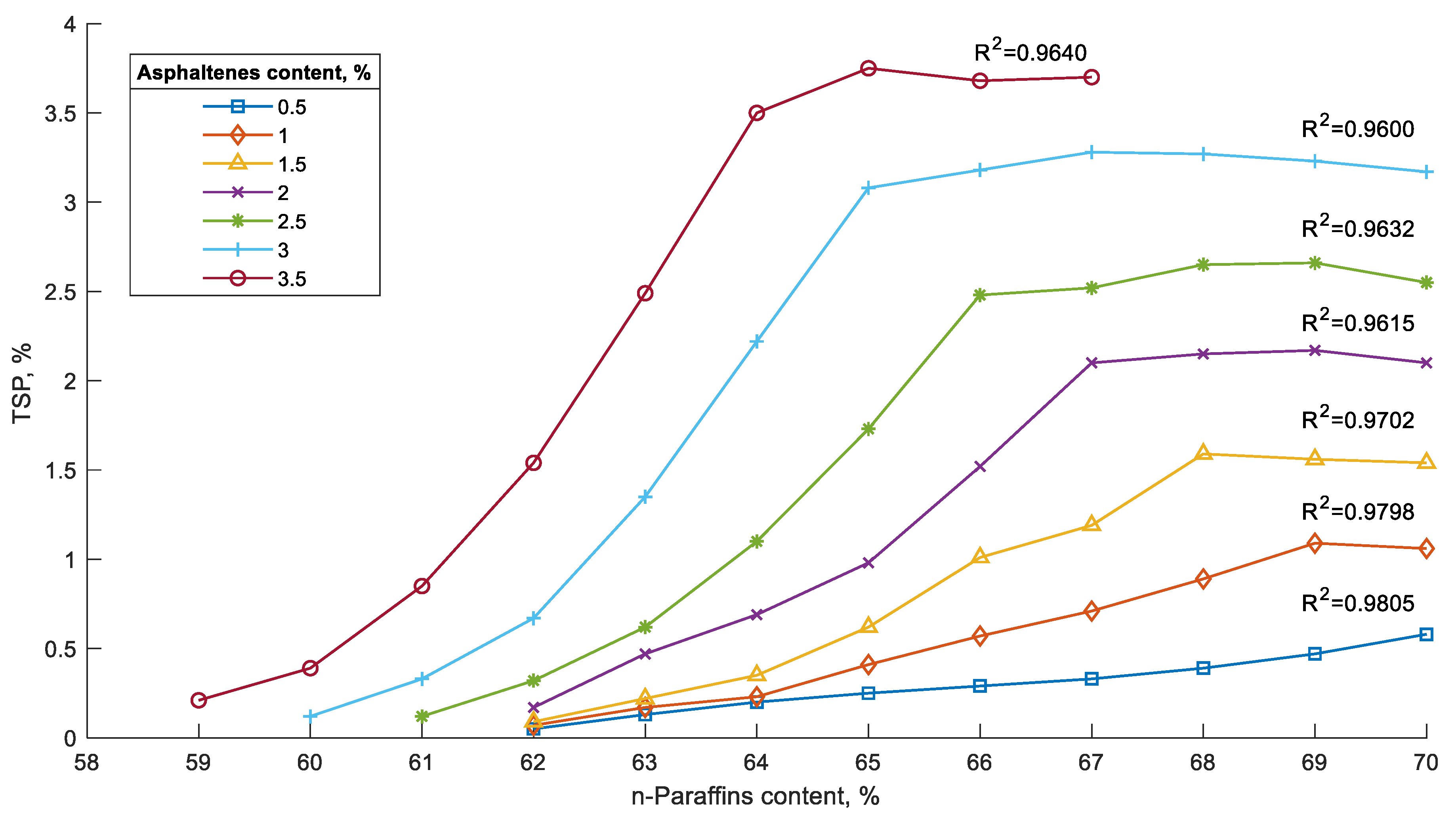
Also, based on production and experimental data, we carried out studies of the effect of aromatic hydrocarbons on the precipitation of asphaltenes. We found that an increase in the proportion of aromatic hydrocarbons reduces sedimentation. However, the effect of paraffins on the precipitation of asphaltenes has not been considered; therefore, more detailed studies in this direction are required [36,37]. We obtained and substantiated the dependences of the effect of n-paraffins (from 55 to 70 wt. %) at specific values of asphaltenes (0.5, 1, 1.5, 2, 2.5, 3, 3.5 wt. %) on the basis of experimental studies [38].
In this article, the task is to expand the possibilities of applying the results obtained using widely tested methods of machine learning [39]. All these make it possible to determine the risks of incompatibility in the considered range (but not at specific values of asphaltenes and n-paraffins) with a high level of confidence.
A fairly large set of classification/regression algorithms is tested to choose the most efficient for the problem to be investigated. The tested methods can be divided into three families: decision trees, k-nearest neighbors (k-NN), multiple linear regression, and function of two variables. They are briefly described as follows.
Braidotti et al. [40] applied machine learning methods (such as decision trees, k-NN, and support vector machine) in their study. Based on their research, the best choice was represented by package decision trees, which showed very good accuracy for methods of classifying and defining damaged compartments. To solve other problems, they recommended giving preference to weighted k-NN, which ensured better accuracy of the prediction scenario.
Codjo et al. [41] used various machine learning methods to identify certain features of the investigated object degradation. Various methods of controlled learning were applied. A comparison of classifiers and methods showed that logistics regression and decision tree approaches were robust binary classification tools with an accuracy of 97.917% and 99.884%, respectively, while the k-NN method cannot provide accurate predictions. Due to the processing of the results by using modern machine learning methods, it is possible to expand the application of the results obtained.
Zhang et al. [42] performed an experiment to simulate the exhaust emissions from ships. The sulfur content prediction model has made it possible to effectively predict the sulfur content in marine fuel oil. The paper discusses the use of a deep neural network to improve the accuracy of predicting the sulfur content in marine residual fuel.
The literature analysis showed that there is a global problem: approximately 15% of NOx emissions and 4% to 9% of SO2 emissions are caused by shipping [43]. About 70% of exhaust gases are discharged into the maritime atmosphere at a distance of less than 400 km from the land, causing serious air pollution in coastal areas, especially around ports with a high flow of cargo [44,45,46,47,48]. Sulfur contained in marine fuel oil leads to the formation of large amounts of SO2 as a result of chemical reactions occurring during engine operation, and the amount of SO2 emitted is directly related to the sulfur content in the marine fuel [49]. The tightening of requirements for the sulfur content has shown that the available knowledge is insufficient, and this direction of research is extremely urgent.
Based on the current state of the problem and possible solution methods, it can be concluded that the use of machine learning tools for predicting and modeling the composition of marine fuels is relevant. However, to date, there is no specific method that allows one to accurately determine the characteristics of incompatibility of fuels. In addition, the accuracy of using various machine learning methods is highly dependent on the input data.
The lack of exact dependencies on the influence of the composition of residual fuel oils on sediment formation due to the manifestation of incompatibility allows us to identify a gap in the studies. Many researchers limit themselves only to general recommendations, and this problem has not been fully resolved in any way. Understanding and correct use of machine learning methods will allow you to develop an effective tool and significantly improve forecast accuracy.
2. Materials and Methods
Several methods of machine learning have been considered for developing a practical robust tool, which can be used to determine sediment formation based on the results of experimental studies of the influence of n-paraffins and asphaltenes on the compatibility of marine residual fuels.
The first method considered is multiple linear regression. This model is one of the most important and widely used regression techniques. One of its advantages is the ease of interpretation of the results.
The mathematical model based on graphs—the decision tree—is considered. This model defines the decision making process in such a way that every possible decision, the preceding and subsequent events or other decisions, and the consequences of each final decision are represented. The decision tree is a well-known non-parametric controlled algorithm based on binary solutions. Decision trees can be used for both classification and regression (providing a piecewise approximation of the response function). The decision-making process takes the form of a tree or graph, starting from a zero vertex and then moving from one vertex to another according to the predictors’ values of the predictors (the leaves are the predicted answer). A typical decision tree structure is shown in Figure 1. Starting with the route, decisions are made from two possible directions according to the value of one predictor xj. A similar process is performed in each passed node along with the tree structure until a decision-by-decision sheet corresponding to the answer class is reached.
Decision trees are trained using a dataset that provides relationships between predictors and responses, simulating the relationship between them. In this paper, a single decision tree method is adopted by using the Gini Diversity Index as a measure of taking into account the separation criteria [50]. All predictors are tested in each node to select one that maximizes the benefit of the separation criterion.
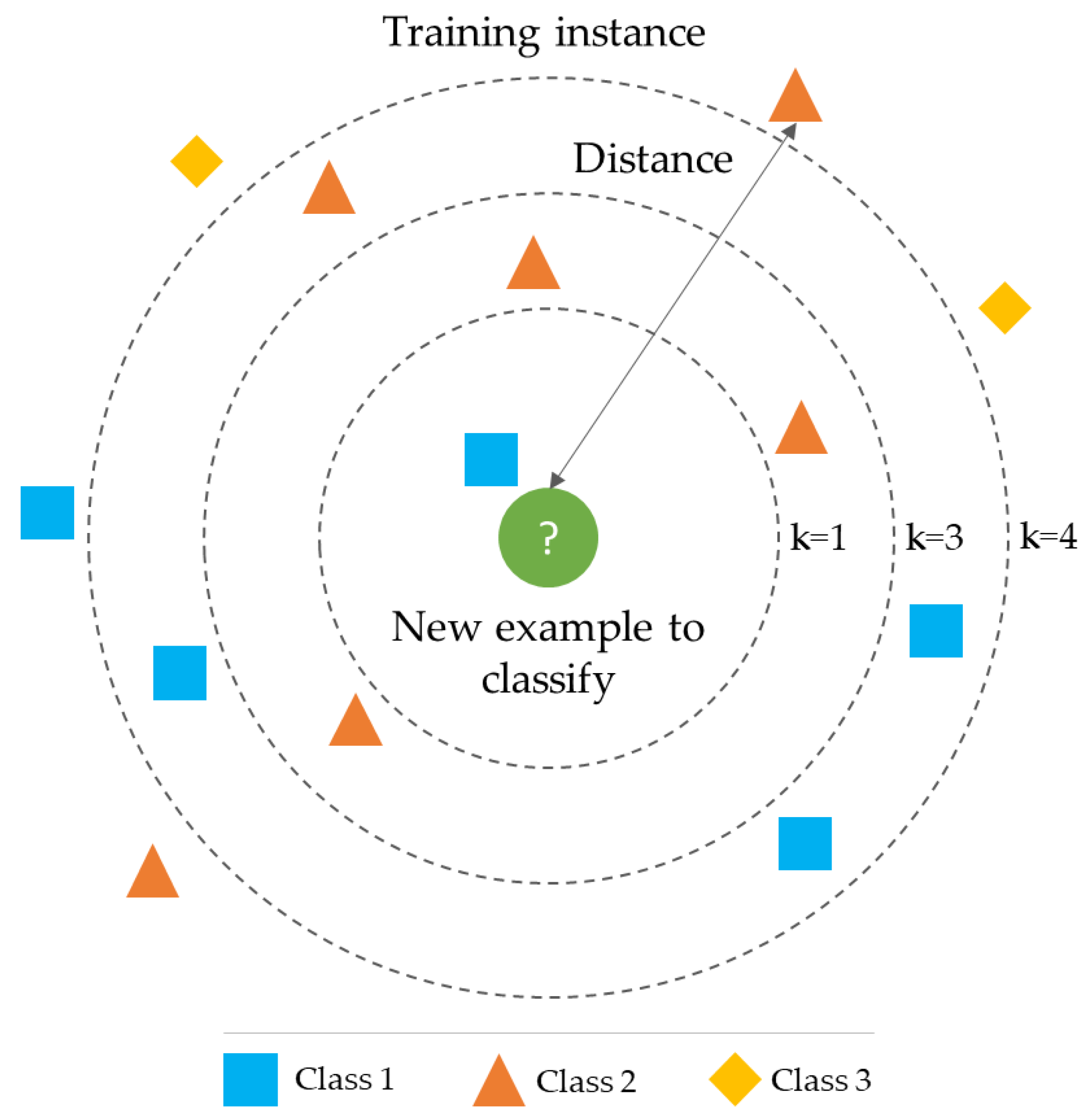
The k-NN method is also used to solve the classification problem. It assigns objects to a class that belongs to most of k of its nearest neighbors in a multidimensional feature space. The number k is the number of neighboring objects in the feature space that are compared with the classified object. In other words, if k = 4, then each object is compared with four neighbors. The method is widely used in Data Mining technologies.
This algorithm can be divided into two simple phases: learning and classification. During training, the algorithm remembers the observation feature vectors and their class labels (i.e., examples). Also, the algorithm parameter k is set, which sets the number of “neighbors” that will be used in the classification. During the classification phase, a new object is presented for which no class label has been set. The k-nearest preliminary classified observations are determined for it. Then a class is selected to which most of the k-nearest neighbor examples belong, and the object being classified belongs to the same class [51] (Figure 2).
The circle on Figure 2 represents the object that needs to be classified into one of the two classes “triangles” and “squares”. If we choose k = 3, then out of the three nearest objects, two will turn out to be “triangles” and one “square”.
The Python programming language is used to implement the aforementioned methods. In addition, to solve the problem, the mathematical method of finding a function of two variables by approximation in the Matlab program is employed.
3. Results
In the present study, marine residual fuels of the following grades are used:
- Sample No.1—Compound oils grade A type 1(KMC).
- Sample No.2—Fuel for TSU-80 marine installations (RMD-80).
- Sample No.3—Fuel for TSU-380 marine installations (RMG-380).
- Sample No.4—Residual oil fuel M-100, low ash (RK-700).
The main physical and chemical indicators of the fuels have been determined, which are presented in Table 1.
Using SARA analysis, the group composition of the presented fuels was determined (Table 2), after which the fuel mixtures were prepared according to the experiment plan [38,44].
Seven series of laboratory tests have been carried out based on the method proposed by the authors [52] to determine the compatibility and stability of marine residual fuels. The influence of n-paraffins from 55 to 70 wt. % is determined when the asphaltene content ranges from 0.5 to 3.5 wt. % with a step of 0.5% and the dependencies shown in Figure 3.
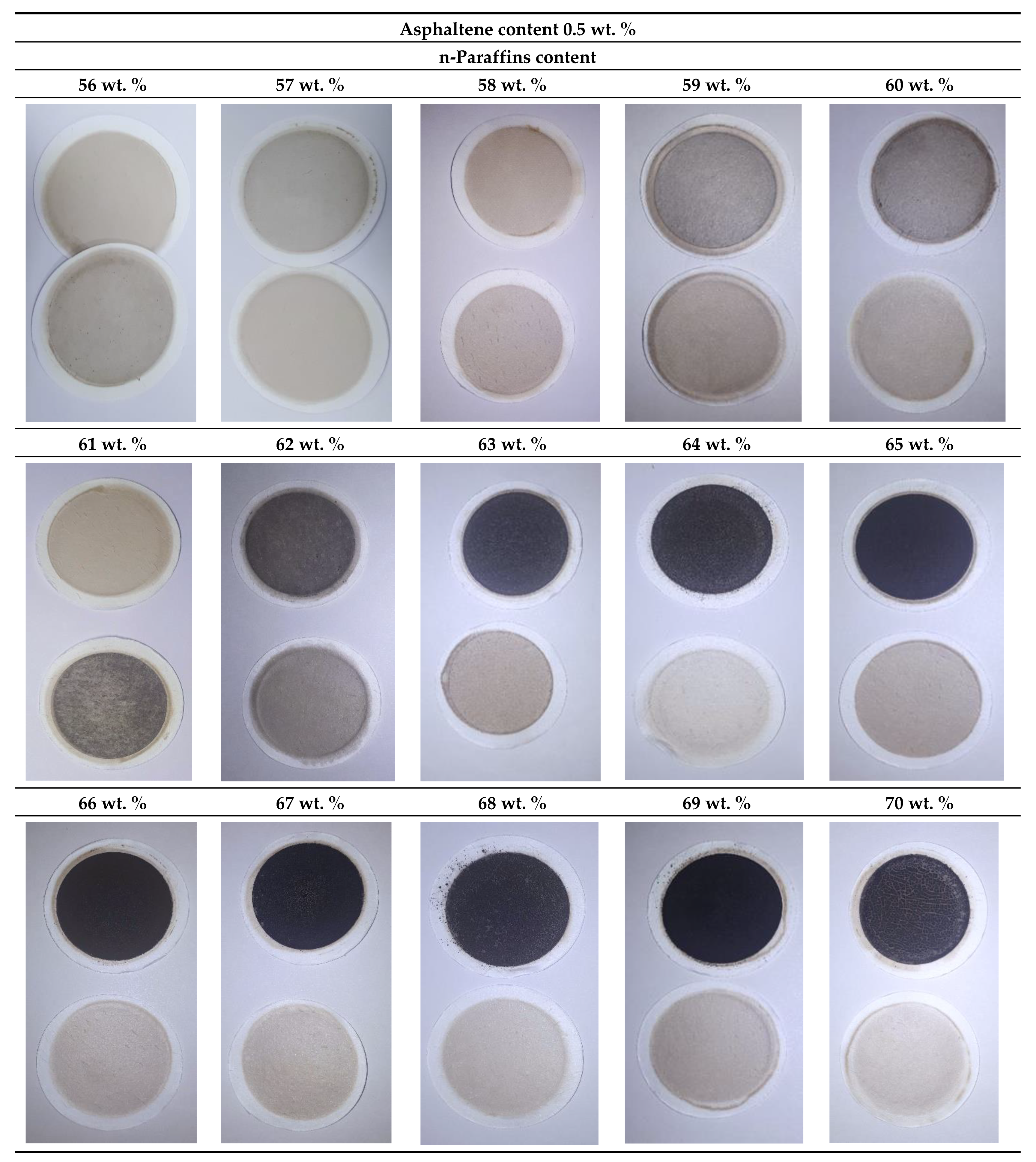
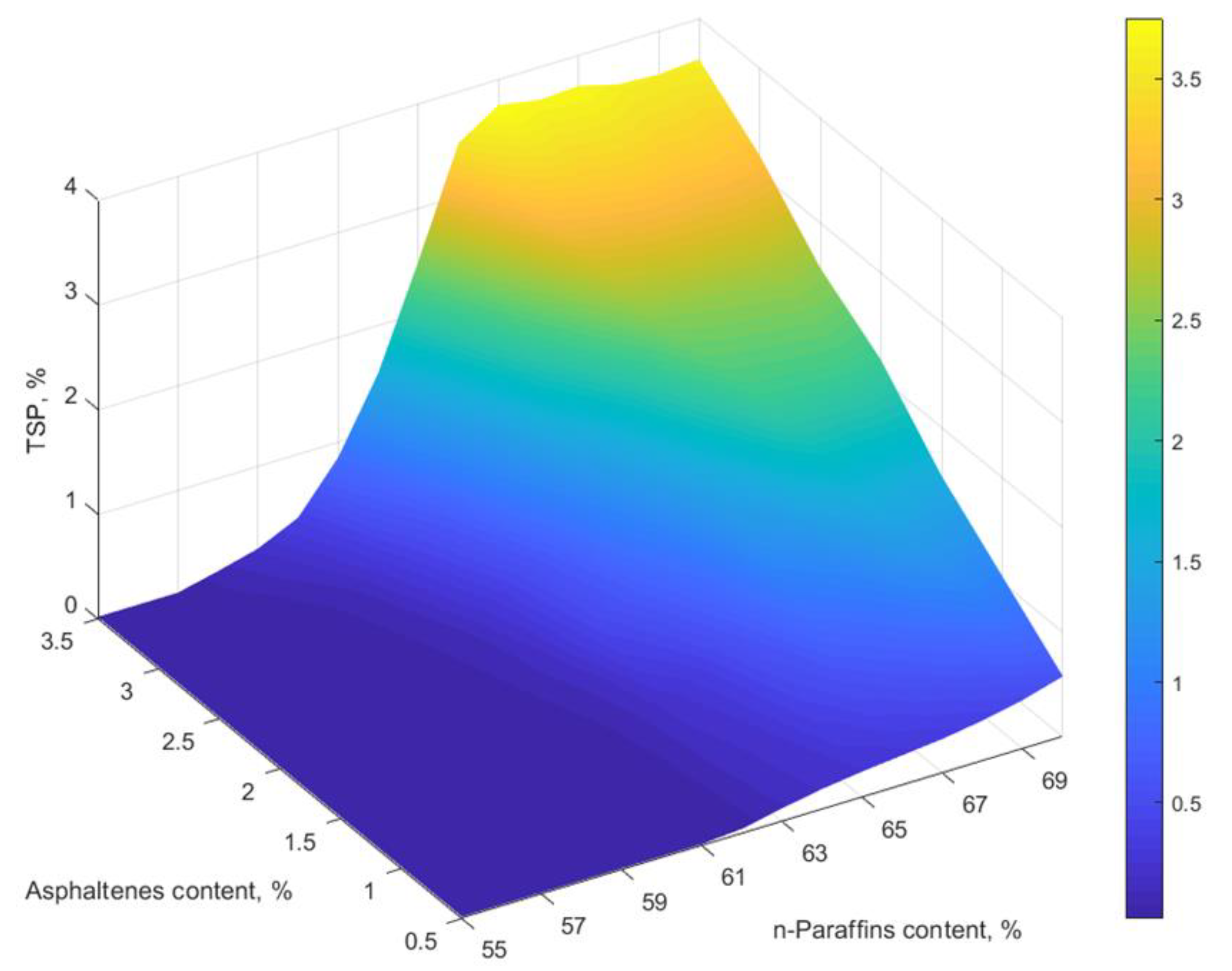
A total of 112 different fuel mixtures with the required composition are prepared and laboratory tests are performed to determine the TSP content. Figure 4 shows filters for one series of tests with an asphaltene content of 0.5 wt. % and n-paraffins from 56 to 70 wt. %, as an example [38,52,53]. Even visually, it is possible to determine the incompatibility of fuel compositions with n-paraffin content of 63 to 70 wt. %, where there is a large amount of total sediment in the upper filters. Three-dimensional visualization of the obtained experimental results is shown in Figure 5.
A three-dimensional visualization of the present results is presented in Figure 4.
Table 3 shows the numerical interpretation of the three-dimensional model due to the influence of asphaltenes and n-paraffins on sediment formation.
Based on the obtained experimental data, it is possible to determine the dependences of the influence of fuel mixture composition on sedimentation. However, the presented data only describe dependencies on the specific content of the fuel composition, which is difficult to apply in practice. Therefore, it is necessary to develop a practical robust tool to determine the sedimentation activity at different values of n-paraffin and asphaltene in the ranges considered.
The following methods are considered to process the experimental data for the development of the numerical tool:
- linear regression,
- decision tree,
- k-NN,
- finding a function of two variables by approximation.
Using a linear regression model, weights for the parameters x and y are found. Based on this, a linear regression formula is derived that allows combining the results of all experiments. The linear regression formula for the parameters analyzed parameters:
z = 0.66673469∙x + 0.20424176∙y
The determinant coefficient R2 of this formula is 0.772.
Using the machine learning model “decision tree”, it is also possible to achieve a higher coefficient of determination R2 = 0.910. In the visualization of the decision tree model, it can be seen how branches and leaves are divided by parameters and values. This model can be used to predict other results depending on parameters x and y.
By finding the function of the two variables by approximation, a calculation program has been developed based on the obtained data, which will make it possible to obtain the result in a convenient format under certain boundary conditions. The pseudo-programming Procedure 1 is shown below.
| Procedure 1. Approximation of two variables |
| Input: n, m, data for i = 1 to ndo for j = 1 to m do Polyfit()the coefficients of the fifth-order polynomial Linspace() Polyval() calculating the ordinates of the approximating polynomial end for For each k = Ipolynomialcoefficients by xi Endfor |
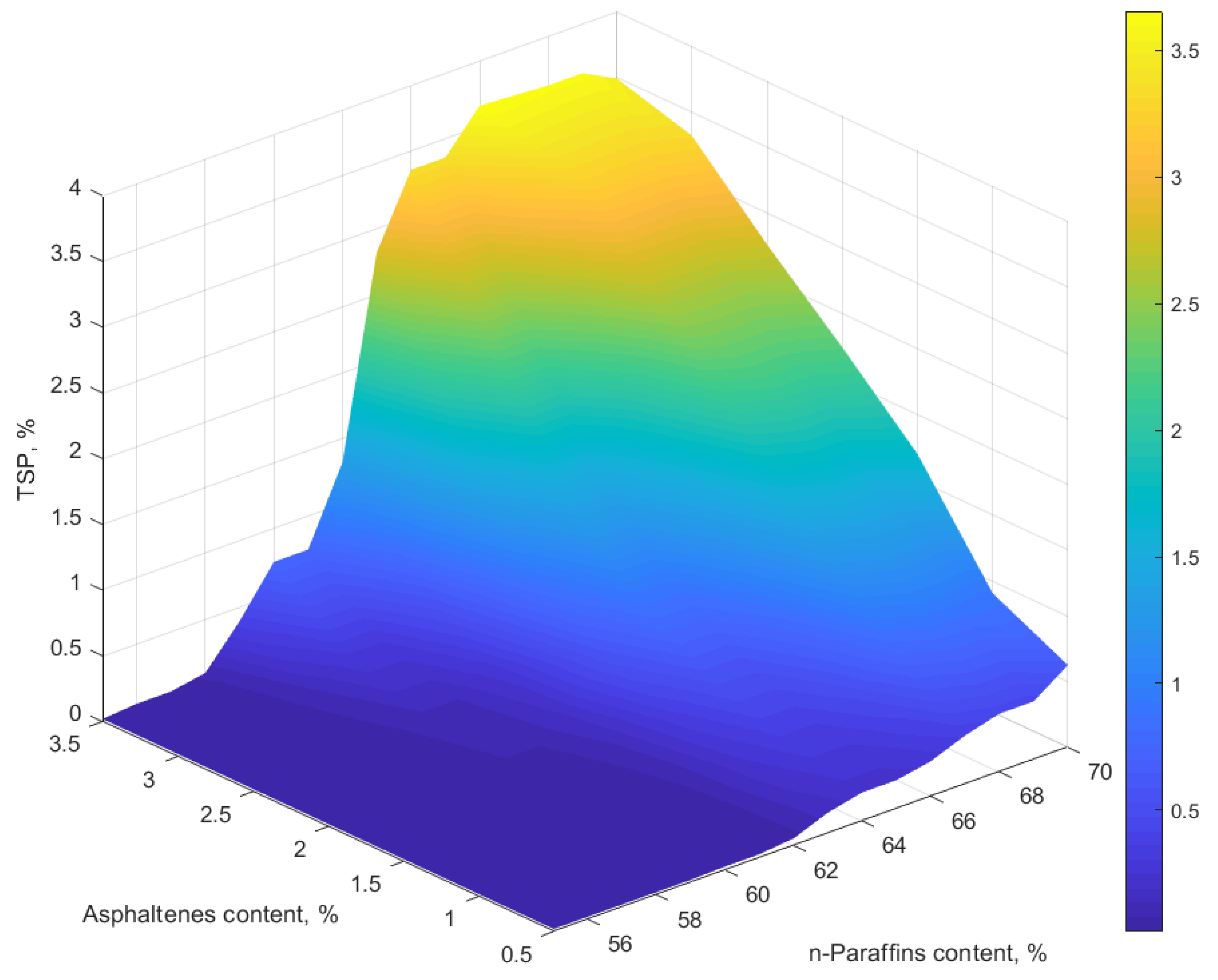
In order to define the unknown function of two variables Z = f(X,Y), it is necessary to construct graphs for known values Y from the data presented as a table. Then construct the most accurate trend line (5th degree polynomial with approximation value above R2 = 0.990). The polynomial trend line in the 4th degree gives less accuracy of the approximation, and in the 6th degree it is identical, as in the 5th degree. To obtain a more accurate model, the data range of the corresponding n-paraffin content from 57 to 70 wt. % is considered. The next step is to determine the coefficients of the polynomial and to create an equation Z = f(X) for each curve. The following is the function Z = f(X,Y) and the definition of polynomial coefficients for the function of two variables. Thus, introducing any values of n-paraffins (X) between 55 and 70 and asphaltenes (Y) between 0.5 and 3.5 makes it possible to define TSP values. The results of the calculations are presented in Figure 6 and Table 4.
Based on the k-NN method, a program in Python is developed for calculating the TSP indicator in the fuel mixture from the results of the received experimental data. The program Procedure 2 is shown as follows.
| Procedure 2. k-NN method |
| Input: import pandas as pd from sklearn.neighbors import KNeighborsRegressor from sklearn.preprocessing import StandardScaler from sklearn.metrics import r2_score df = pd.read_csv(‘data.csv’, sep = ‘;’) X = df[[‘x’, ‘y’]] z = df[‘z’] scaler = StandardScaler()Normalized by StandardScaler X_sc = scaler.fit_transform(X) model_knn = KNeighborsRegressor(n_neighbors = 4) model_knn.fit(X_sc, z) z_pred = model_knn.predict(X_sc) r2_score(z, z_pred) x_new, y_newinput new variables new = scaler.transform([[x_new, y_new]]) model_knn.predict(new) array([0.02]) df[‘z_pred’] = z_pred df.to_csv(‘z_pred.csv’, sep = ‘;’, decimal = ‘,’) |
To increase the numerical precision, normalization is performed and four neighbors are taken, i.e., k = 4. With an increase in the coefficient k, the accuracy of calculations will decrease due to the insufficient data set. The essence of the method is the classification of objects that belong to a larger number of nearest neighbors in a multidimensional feature space compared to the object being classified. This method is used in Data Mining technologies. Mathematically, this method is based on measuring the minimum distance from the center of the group to each observation (2), for which the length of the vector is determined:
By calculating the length of each vector, when entering the values x and y, the value z is determined by interpolation, based on known data from «neighbors». This model has a high confidence level in the approximation R2 = 0.985.
4. Discussion
This article considers four methods for processing experimental data and obtaining a robust tool applicable in practice: linear regression, decision tree, k-NN, and finding the function of two variables as the approximation. Linear regression showed a low confidence result (R2 = 0.772), and the decision tree method (R2 = 0.910) is not reliable enough to address this issue. Presumably, a larger sample of data is required to construct a more accurate model based on this method.
The relatively accurate predictions are obtained from the methods to find the function of two variables by approximation (R2 = 0.90) and k-NN (R2 = 0.985). It can be noted that the performed calculations of the TSP values by the k-NN method have the greatest error at the boundary maximum values, since neighbors are represented only by groups from opposite sides relative to the data border in the area of maximum values.
On the contrary, in calculations based on a function of two variables, the largest error is observed at a low concentration of n-paraffins and simultaneously at the highest asphaltene values. The trend line is represented by a polynomial function of the 5th degree. Therefore, the beginning of the dependence has a wave form. The amplitude of polynomial function increases with increasing TSP values, so the graph of the function may cross the x-axis. In order to avoid the occurrence of negative values, the obtained data are taken modulo.
The present results show that it is possible to calculate the incompatibility manifestation in the mixing of marine residual fuels in practice. Because of the obtained dependences of the influence of n-paraffins and asphaltenes on the manifestation of incompatibility, it is possible to reduce the risks in advance when constructing the logistic supply chain of fuels to marine fuel terminals and tank farms. The present results can be used to create a numerical model for predicting the sediment content in compounded marine fuels with the required sulfur content.
The change in the symmetrical position of the three-dimensional surface shown in Figure 4, Figure 5 and Figure 6 indicates a change in the dependence between asphaltene and n-paraffin content as well as the corresponding sedimentation. Thus, the asymmetry of the three-dimensional diagrams is the incompatibility degree of residual marine fuels, showing the influence of the presented factors on precipitation [54,55,56,57,58,59].
5. Conclusions
In this study, experiments are performed to determine the physical and chemical characteristics of the fuels. Measurements of the influence of n-paraffins and asphaltenes on the total sediment content have been carried out. By analysis of the experimental results, the main correlations between the composition of the fuel mixture composition and sedimentation are obtained. Various machine learning methods are used in processing the data. In this way, a robust tool has been developed to determine the possibility of incompatibility occurrence in the mixing of various types of marine residual fuels.
The absence of requirements in the international standard ISO 8217 for the content of asphaltenes in marine residual fuels preserves the risks of incompatibility. In this regard, active sediment formation can cause not only environmental problems, but technical problems as well. During the operation of marine engines, a high sediment content can lead to a breakdown of the entire fuel system and clogging of filters, which is a substantial threat to normal operation and personnel safety, especially if a breakdown occurs during navigation far from berths and ports and/or in bad weather conditions. It is proposed to regulate this parameter. This will allow shipowners and buyers to assess in advance the risks of incompatibilities and thus maintain fuel quality.
In future studies, it is possible to carry out experiments to determine the sulfur content of the exhaust gases as well as in the sediment itself, depending on the calculated incompatibility parameters, to create a model to predict SO2 concentration in the exhaust gases of ships. In addition, the deep neural network will be enhanced in order to improve the accuracy of its predictions and calculations
6. Patents
Method of determining compatibility and stability of fuel mixture components. Available online: https://new.fips.ru/ofpstorage/Doc/IZPM/RUNWC1/000/000/002/733/748/%D0%98%D0%97-02733748-00001/document.pdf (accessed on 23 September 2021).
Program for calculating kinematic viscosity, density, sulfur, and water content for a mixture of crude oil and petroleum products. Available online: https://new.fips.ru/ofpstorage/Doc/PrEVM/RUNWPR/000/002/020/613/357/2020613357-00001/document.pdf (accessed on 23 September 2021).
Author Contributions
Conceptualization, R.S., I.B. and S.I.; methodology, I.B.; software, R.S. and I.B.; validation, S.I.; formal analysis, I.B.; investigation, R.S., I.B., S.I. and M.C.O.; resources, R.S. and I.B.; data curation, R.S. and I.B.; writing—original draft preparation, R.S., I.B. and S.I.; writing—review and editing, R.S., I.B., S.I. and M.C.O.; visualization, S.I. and M.C.O.; supervision, R.S.; project administration, R.S. All authors have read and agreed to the published version of the manuscript.
Funding
The research was performed at the expense of the subsidy for the state assignment in the field of scientific activity for 2021: FSRW-2020-0014.
Institutional Review Board Statement
Not applicable.
Informed Consent Statement
Not applicable.
Data Availability Statement
Not applicable.
Acknowledgments
The authors thank Saint Petersburg Mining University for enabling the laboratory experiments. The investigations were carried out using the equipment of the Scientific Center “Issues of Processing Mineral and Technogenic Resources” and Educational Research Center for Digital Technology of the Saint Petersburg Mining University.
Conflicts of Interest
The authors declare no conflict of interest.
Abbreviations
| GOST | Russian government standard |
| ISO | International organization for standardization |
| IMO | International Maritime Organization |
| k-NN | k-nearest neighbors |
| SARA | Saturate, aromatic, resin, and asphaltene |
| TSA | Total sediment accelerated |
| TSP | Total sediment potential |
References
- 2050 Long-Term Strategy. Available online: https://ec.europa.eu/clima/eu-action/climate-strategies-targets/2050-long-term-strategy_en (accessed on 11 October 2021).
- Concepts for the Development of Hydrogen Energy in the Russian Federation. Available online: http://government.ru/docs/42971/ (accessed on 11 October 2021).
- On Approval of a Comprehensive Plan to Improve the Energy Efficiency of the Russian Economy. Available online: http://static.government.ru/media/files/rE6AtHAmGYeZUz51fpCeHYfmuyRzUGow.pdf (accessed on 11 October 2021).
- On Introducing a Draft Law on the Use of Subsoil Waste. Available online: http://static.government.ru/media/files/el8BjIdNpygksaGP3td60eqnQ1XvPfwz.pdf (accessed on 11 October 2021).
- Morenov, V.; Leusheva, E.; Buslaev, G.; Gudmestad, O.T. System of comprehensive energy-efficient utilization of associated petroleum gas with reduced carbon footprint in the field conditions. Energies 2020, 13, 4921. [Google Scholar] [CrossRef]
- Bykova, M.V.; Alekseenko, A.V.; Pashkevich, M.A.; Drebenstedt, C. Thermal desorption treatment of petroleum hydrocarbon-contaminated soils of tundra, taiga, and forest steppe landscapes. Environ. Geochem. Health 2021, 43, 2331–2346. [Google Scholar] [CrossRef]
- Litvinenko, V. The role of hydrocarbons in the global energy agenda: The focus on liquefied natural gas. Resources 2020, 9, 59. [Google Scholar] [CrossRef]
- Litvinenko, V.; Meyer, B. Syngas Production: Status and Potential for Implementation in Russian Industry; Springer International Publishing: Cham, Switzerland, 2017; pp. 1–161. [Google Scholar] [CrossRef]
- Zhukovskiy, Y.; Tsvetkov, P.; Buldysko, A.; Malkova, Y.; Stoianova, A.; Koshenkova, A. Scenario Modeling of Sustainable Development of Energy Supply in the Arctic. Resources 2021, 10, 124. [Google Scholar] [CrossRef]
- Korshunov, G.I.; Eremeeva, A.M.; Drebenstedt, C. Justification of the use of a vegetal additive to diesel fuel as a method of protecting underground personnel of coal mines from the impact of harmful emissions of diesel-hydraulic locomotives. J. Min. Inst. 2021, 247, 39–47. [Google Scholar] [CrossRef]
- Statistical Review of World Energy 2021 (70th edition). Available online: https://www.bp.com/content/dam/bp/business-sites/en/global/corporate/pdfs/energy-economics/statistical-review/bp-stats-review-2021-oil.pdf (accessed on 11 October 2021).
- Annual Report 2020. Available online: https://www.opec.org/opec_web/static_files_project/media/downloads/publications/AR%202020.pdf (accessed on 11 October 2021).
- Analysis and Forecast to 2026 (Oil 2021). Available online: https://iea.blob.core.windows.net/assets/1fa45234-bac5-4d89-a532-768960f99d07/Oil_2021-PDF.pdf (accessed on 11 October 2021).
- Schieldrop, B. IMO 2020 Report: Macro & FICC Research; Skandinaviska Enskilda Banken AB Publication: Stockholm, Sweden, 2018. [Google Scholar]
- Fetisov, V.; Mohammadi, A.H.; Pshenin, V.; Kupavykh, K.; Artyukh, D. Improving the economic efficiency of vapor recovery units at hydrocarbon loading terminals. Oil Gas Sci. Technol. Rev. IFP Energ. Nouv. 2021, 76, 38. [Google Scholar] [CrossRef]
- Fetisov, V.; Pshenin, V.; Nagornov, D.; Lykov, Y.; Mohammadi, A.H. Evaluation of pollutant emissions into the atmosphere during the loading of hydrocarbons in marine oil tankers in the Arctic region. J. Mar. Sci. Eng. 2020, 8, 917. [Google Scholar] [CrossRef]
- IMO. Reduction of GHG Emissions from Ships—Third IMO GHG Study 2014—Final Report; International Maritime Organization: London, UK, 2015. [Google Scholar]
- IMO. Annex VI Prevention of Air Pollution from Ships of International Convention for the Prevention of Pollution from Ships (MARPOL); International Maritime Organization: London, UK, 2005. [Google Scholar]
- Kunshin, A.A.; Dvoynikov, M.V.; Blinov, P.A. Topology and dynamic characteristics advancements of liner casing attachments for horizontal wells completion. In Proceedings of the VI Youth Forum of the World Petroleum Council–Future Leaders Forum; St. Petersburg, Russia, 23–28 June 2019, Taylor & Francis: London, UK, 2019; pp. 376–381. [Google Scholar]
- Li, C.; Yuan, Z.; Ou, J.; Fan, X.; Ye, S.; Xiao, T.; Shi, Y.; Huang, Z.; Ng, S.K.; Zhong, Z.; et al. An AIS-based high-resolution ship emission inventory and its uncertainty in Pearl River Delta region, China. Sci. Total Environ. 2016, 573, 1–10. [Google Scholar] [CrossRef]
- Liu, T.K.; Chen, Y.S.; Chen, Y.T. Utilization of vessel automatic identification system (AIS) to estimate the emission of air pollutant from merchant vessels in the port of Kaohsiung. Aerosol Air Qual. Res. 2019, 19, 2341–2351. [Google Scholar] [CrossRef]
- Miola, A.; Ciuffo, B.; Giovine, E.; Marra, M. Regulating Air Emissions from Ships: The State of the Art on Methodologies, Technologies and Policy Options; Publications Office of the European Union: Luxembourg, 2010. [Google Scholar]
- Lindstad, H.E.; Rehn, C.F.; Eskeland, G.S. Sulphur abatement globally in maritime shipping. Transp. Res. Part D Transp. Environ. 2017, 57, 303–313. [Google Scholar] [CrossRef] [Green Version]
- Kondrasheva, N.K.; Rudko, V.A.; Nazarenko, M.Y.; Gabdulkhakov, R.R. Influence of parameters of delayed asphalt coking process on yield and quality of liquid and solid-phase products. J. Min. Inst. 2020, 241, 97–104. [Google Scholar] [CrossRef]
- Gulvaeva, L.A.; Khavkin, V.A.; Shmelkova, O.I.; Mitusova, T.N.; Ershov, M.A.; Lobashova, M.M.; Nikulshin, P.A. Production technology for low-sulfur high-viscosity marine fuels. Chem. Technol. Fuels Oils 2019, 54, 759–765. [Google Scholar] [CrossRef]
- Dvoynikov, M.; Buslaev, G.; Kunshin, A.; Sidorov, D.A.; Kraslawski, A.; Budovskaya, M. New concepts of hydrogen production and storage in Arctic region. Resources 2021, 10, 3. [Google Scholar] [CrossRef]
- Nguyen, V.T.; Rogachev, M.K.; Aleksandrov, A.N. A new approach to improving efficiency of gas-lift wells in the conditions of the formation of organic wax deposits in the Dragon field. J. Petrol. Explor. Prod. Technol. 2020, 10, 3663–3672. [Google Scholar] [CrossRef]
- Bai, J.; Jin, X.; Wu, J.T. Multifunctional anti-wax coatings for paraffin control in oil pipelines. Pet. Sci. 2019, 16, 619–631. [Google Scholar] [CrossRef] [Green Version]
- Coutinho, J.A.P.; Edmonds, B.; Moorwood, T.; Szczepanski, R.; Zhang, X. Reliable wax predictions for flow assurance. Energy Fuels 2006, 20, 1081–1088. [Google Scholar] [CrossRef]
- Kelbaliev, G.I.; Rasulov, S.R.; Ilyushin, P.Y.; Mustafaeva, G.R. Crystallization of paraffin from the oil in a pipe and deposition of asphaltene–paraffin substances on the pipe walls. J. Eng. Phys. Thermophy. 2018, 91, 1227–1232. [Google Scholar] [CrossRef]
- Rogachev, M.K.; Nguyen, V.T.; Aleksandrov, A.N. Technology for preventing the wax deposit formation in gas-lift wells at offshore oil and gas fields in Vietnam. Energies 2021, 14, 5016. [Google Scholar] [CrossRef]
- Wiehe, I.A.; Yarranton, H.W.; Akbarzadeh, К.; Rahimi, P.M.; Teclemariam, A. The paradox of asphaltene precipitation with normal paraffins. Energy Fuels 2005, 19, 1261–1267. [Google Scholar] [CrossRef]
- Prakoso, A.; Punase, A.; Klock, K.; Rogel, E.; Ovalles, C.; Hascakir, B. Determination of the stability of asphaltenes through physicochemical characterization of asphaltenes. In Proceedings of the SPE Western Regional Meeting, Anchorage, AK, USA, 23 May 2016; pp. 1–20. [Google Scholar]
- Wiehe, I.A.; Kennedy, R.J. The oil compatibility model and crude oil incompatibility. Energy Fuels 2000, 14, 56–59. [Google Scholar] [CrossRef]
- Mitusova, T.N.; Kondrasheva, N.K.; Lobashova, M.M.; Ershov, M.A.; Rudko, V.A. Influence of dispersing additives and blend composition on stability of marine high-viscosity fuels. J. Min. Inst. 2017, 228, 722–725. [Google Scholar]
- Stratiev, D.; Dinkov, R.; Shishkova, I.; Yordanov, D. Can we manage the process of asphaltene precipitation during the production of IMO 2020 fuel oil? Erdoel Erdgas Kohle/EKEP 2020, 12, 32–39. [Google Scholar]
- Stratiev, D.; Russell, C.; Sharpe, R.; Shishkova, I.; Dinkov, R.; Marinov, I.; Petkova, N.; Mitkova, M.; Botev, T.; Obryvalina, A.; et al. Investigation on sediment formation in residue thermal conversion based processes. Fuel Process. Technol. 2014, 128, 509–518. [Google Scholar] [CrossRef]
- Sultanbekov, R.; Islamov, S.; Mardashov, D.; Beloglazov, I.; Hemmingsen, T. Research of the influence of marine residual fuel composition on sedimentation due to incompatibility. J. Mar. Sci. Eng. 2021, 9, 1067. [Google Scholar] [CrossRef]
- Boikov, A.; Payor, V.; Savelev, R.; Kolesnikov, A. Synthetic data generation for steel defect detection and classification using deep learning. Symmetry 2021, 13, 1176. [Google Scholar] [CrossRef]
- Braidotti, L.; Valčić, M.; Prpić-Oršić, J. Exploring a flooding-sensors-agnostic prediction of the damage consequences based on machine learning. J. Mar. Sci. Eng. 2021, 9, 271. [Google Scholar] [CrossRef]
- Codjo, E.L.; Zad, B.B.; Toubeau, J.-F.; François, B.; Vallée, F. Machine learning-based classification of electrical low voltage cable degradation. Energies 2021, 14, 2852. [Google Scholar] [CrossRef]
- Zhang, Z.; Zheng, W.; Li, Y.; Cao, K.; Xie, M.; Wu, P. Monitoring sulfur content in marine fuel oil using ultraviolet imaging technology. Atmosphere 2021, 12, 1182. [Google Scholar] [CrossRef]
- Eyring, V.; Isaksen, I.S.A.; Berntsen, T.; Collins, W.J.; Corbett, J.J.; Endresen, O.; Grainger, R.G.; Moldanova, J.; Schlager, H.; Stevenson, D.S. Transport impacts on atmosphere and climate: Shipping. Atmos. Environ. 2010, 44, 4735–4771. [Google Scholar] [CrossRef]
- Zhao, J.; Fan, J.; Zhang, B.; Shi, Y. Satellite remote-sensing monitoring technology and the research advances of SO2 in the atmosphere. J. Saf. Environ. 2012, 4, 166–169. [Google Scholar]
- Yan, H.; Chen, L.; Tao, J.; Han, D.; Su, L.; Yu, C. SO2 long-term monitoring by satellite in the Pearl River Delta. J. Remote Sens. 2012, 2, 390–404. [Google Scholar]
- Huaxiang, S.; Minhua, Y. Effectiveness evaluation of SO2 emission reduction in Guizhou Province. Earth Environ. 2014, 5, 319–327. [Google Scholar]
- Huaxiang, S.; Minhua, Y. Analysis on effectiveness of SO2 emission reduction in Guangxi Zhuang Autonomous Region by satellite remote sensing. Chin. J. Environ. Eng. 2015, 3, 1361–1368. [Google Scholar]
- Li, B.; Ju, T.; Zhang, B.; Ge, J.; Zhang, J.; Tang, H. Satellite remote sensing monitoring and analysis of the causes of temporal and spatial variation characteristics of atmospheric SO2 Concentration in Tianshui. Environ. Monit. China 2016, 2, 134–140. [Google Scholar]
- Li, C. Emissions Characteristics and Future Trends of Non-Road Mobile Sources in China. Master Thesis, South China University, Guangdong, China, 2017. [Google Scholar]
- Breiman, L.; Friedman, J.; Olshen, R.A.; Stone, C.J. Classification and Regression Trees; CRC Press: Boca Raton, FL, USA, 1984. [Google Scholar]
- Noteworthy the Journal Blog. A Quick Introduction to K-Nearest Neighbors Algorithm. Available online: https://blog.usejournal.com/a-quick-introduction-to-k-nearest-neighbors-algorithm-62214cea29c7 (accessed on 11 October 2021).
- Nutskova, M.V.; Dvoynikov, M.V.; Budovskaya, M.E.; Sidorov, D.A.; Pantyukhin, A.A. Improving energy efficiency in well construction through the use of hydrocarbon-based muds and muds with improved lubricating properties. J. Phys. Conf. Ser. 2021, 1728, 012031. [Google Scholar] [CrossRef]
- Method of Determining Compatibility and Stability of Fuel Mixture Components. Available online: https://new.fips.ru/ofpstorage/Doc/IZPM/RUNWC1/000/000/002/733/748/%D0%98%D0%97-02733748-00001/document.pdf (accessed on 11 October 2021).
- Program for Calculating Kinematic Viscosity, Density, Sulfur and Water Content for a Mixture of Crude Oil and Petroleum Products. Available online: https://new.fips.ru/ofpstorage/Doc/PrEVM/RUNWPR/000/002/020/613/357/2020613357-00001/document.pdf (accessed on 11 October 2021).
- Savchenkov, S.; Kosov, Y.; Bazhin, V.; Krylov, K.; Kawalla, R. Microstructural Master Alloys Features of Aluminum–Erbium System. Crystals 2021, 11, 1353. [Google Scholar] [CrossRef]
- Leusheva, E.L.; Morenov, V.A. Development of combined heat and power system with binary cycle for oil and gas enterprises power supply. Neft. Khozyaystvo-Oil Ind. 104–106. [CrossRef]
- Filatova, I.; Nikolaichuk, L.; Zakaev, D.; Ilin, I. Public-private partnership as a tool of sustainable development in the oil-refining sector: Russian case. Sustainability 2021, 13, 5153. [Google Scholar] [CrossRef]
- Bazhin, V.Y.; Savchenkov, S.A.; Kosov, Y.I. Specificity of the titanium-powder alloying tablets usage in aluminium alloys. Non-Ferrous Met. 2016, 2, 52–56. [Google Scholar] [CrossRef]
- Sharikov, Y.V.; Sharikov, F.Y.; Krylov, K.A. Mathematical Model of Optimum Control for Petroleum Coke Production in a Rotary Tube Kiln. Theor. Found. Chem. Eng. 2021, 55, 711–719. [Google Scholar] [CrossRef]
Figure 1.
Example of a decision tree.
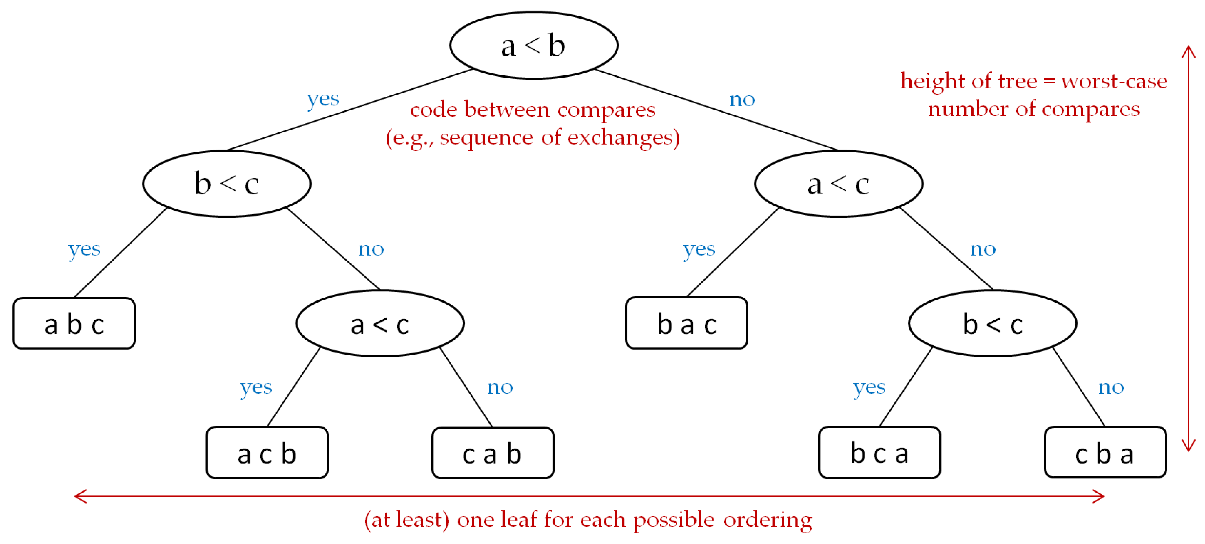
Figure 2.
K-NN representation [51].
Figure 2.
K-NN representation [51].

Figure 3.
Influence of n-paraffins and asphaltenes on the total sediment content.

Figure 4.
Filters after TSP determination at an asphaltene content of 0.5 wt. %.

Figure 5.
Three-dimensional visualization of the obtained experimental data model on the influence of n-paraffins and asphaltenes on incompatibility manifestation.
Figure 5.
Three-dimensional visualization of the obtained experimental data model on the influence of n-paraffins and asphaltenes on incompatibility manifestation.

Figure 6.
Three-dimensional model visualization based on finding the function of two variables by approximation method.
Figure 6.
Three-dimensional model visualization based on finding the function of two variables by approximation method.
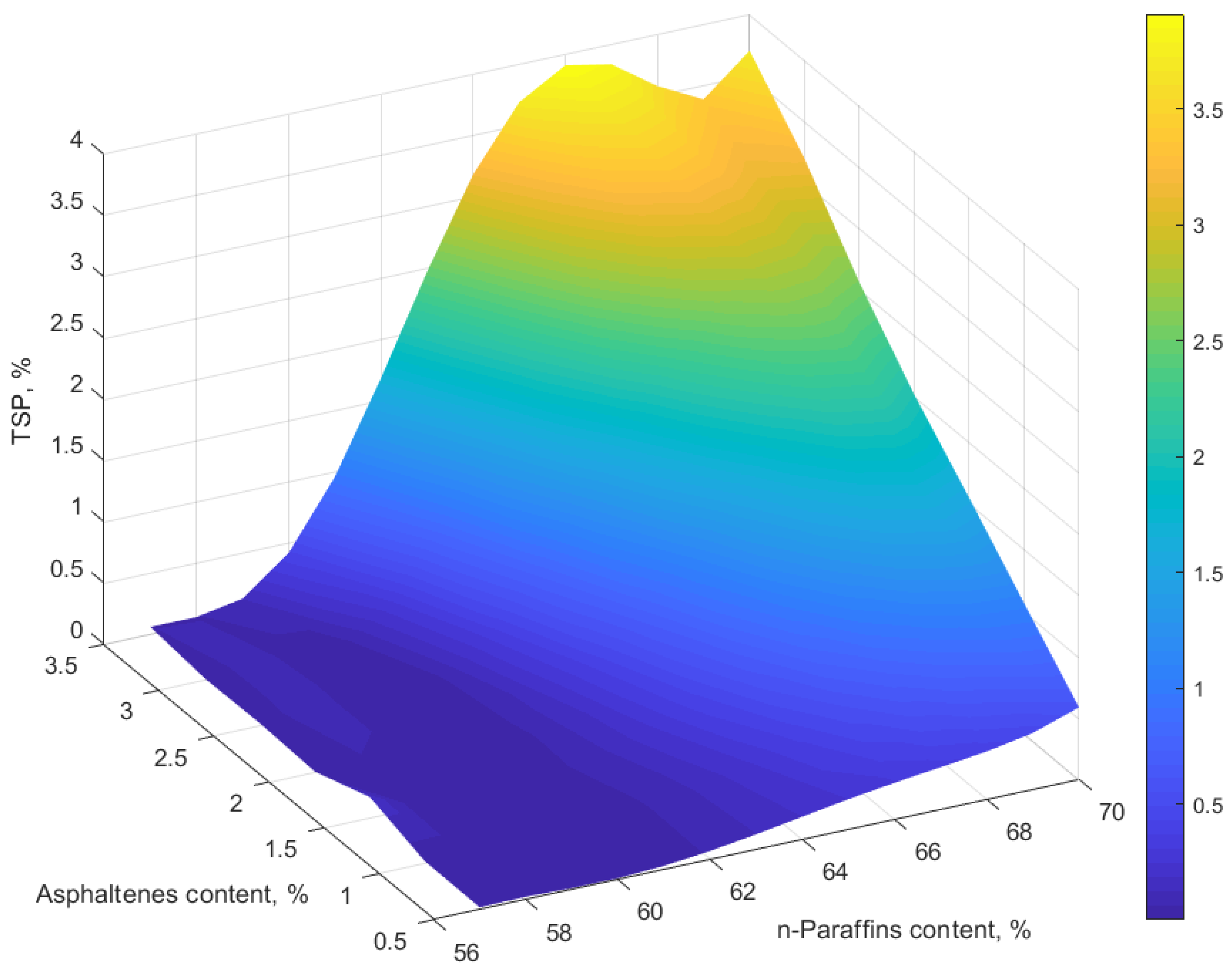
Figure 7.
Three-dimensional visualization based on k-NN.

Table 1.
Quality indicators of residual fuels [38].
Table 1.
Quality indicators of residual fuels [38].
| No. | Indicator Name | Unit of Measurement | Regulation of the Test Method | Result | |||
|---|---|---|---|---|---|---|---|
| Sample No.1 | Sample No.2 | Sample No.3 | Sample No.4 | ||||
| 1 | Density at 15 °C | kg/m3 | ISO 12185 | 833.5 | 901.0 | 956.0 | 976.0 |
| 2 | Kinematic viscosity at 50 °C | mm2/s | GOST 33 ISO 3104 | 12.1 | 34.5 | 321.5 | 680.1 |
| 3 | Flashpoint PMCC | °C | GOST R EN ISO 2719 | 181.0 | 110.0 | 98.0 | 110.0 |
| 4 | Sulfur mass fraction | % | GOST R 51947 ISO 8754 | 0.004 | 0.046 | 1.276 | 2.668 |
| 5 | Pourpoint | °C | ASTM D 6749 | 26.0 | 10.0 | 16.0 | 20.0 |
| 6 | Mass fraction of water | % | GOST R 51946 ISO 3733 | – | – | 0.05 | 0.1 |
| 7 | Total sediment accelerated (TSA) | % | GOST R 50837.6 ISO 10307-2 | 0.01 | 0.01 | 0.02 | 0.03 |
| 8 | Total sediment potential (TSP) | % | GOST R 50837.6 ISO 10307-2 | 0.01 | 0.01 | 0.02 | 0.04 |
Table 2.
Analysis of the hydrocarbon group composition of fuel samples [38].
Table 2.
Analysis of the hydrocarbon group composition of fuel samples [38].
| Fuel Samples | Asphaltenes, % wt. | n-Alkanes, % wt. | Isoalkane, % wt. | Naphthenes, % wt. | Alkenes, % wt. | Aromatic Hydrocarbons, % wt. | Resins, % wt. |
|---|---|---|---|---|---|---|---|
| No.1 | – | 71.93 | 18.35 | 2.62 | 5.55 | 1.55 | – |
| No.2 | – | 38.68 | 55.09 | 4.95 | – | 1.28 | – |
| No.3 | 2.53 | 54.14 | 22.74 | 5.43 | 0.57 | 14.12 | 0.47 |
| No.4 | 7.15 | 51.15 | 20.71 | 4.37 | 0.41 | 15.70 | 0.51 |
Table 3.
Indicators of the influence of n-paraffins and asphaltenes on sedimentation [38].
Table 3.
Indicators of the influence of n-paraffins and asphaltenes on sedimentation [38].
| n-Paraffins, % | Asphaltenes,% | ||||||
|---|---|---|---|---|---|---|---|
| 0.5 | 1.0 | 1.5 | 2.0 | 2.5 | 3.0 | 3.5 | |
| 55 | 0.02 | 0.02 | 0.02 | 0.02 | 0.02 | 0.02 | 0.02 |
| 56 | 0.02 | 0.02 | 0.02 | 0.02 | 0.02 | 0.02 | 0.02 |
| 57 | 0.02 | 0.02 | 0.02 | 0.02 | 0.02 | 0.02 | 0.02 |
| 58 | 0.02 | 0.02 | 0.02 | 0.02 | 0.02 | 0.02 | 0.11 |
| 59 | 0.02 | 0.02 | 0.02 | 0.03 | 0.02 | 0.05 | 0.21 |
| 60 | 0.02 | 0.02 | 0.02 | 0.04 | 0.06 | 0.12 | 0.39 |
| 61 | 0.02 | 0.02 | 0.04 | 0.08 | 0.12 | 0.33 | 0.85 |
| 62 | 0.05 | 0.07 | 0.09 | 0.17 | 0.32 | 0.65 | 1.54 |
| 63 | 0.13 | 0.17 | 0.22 | 0.47 | 0.62 | 1.28 | 2.49 |
| 64 | 0.20 | 0.23 | 0.35 | 0.69 | 1.10 | 2.22 | 3.50 |
| 65 | 0.25 | 0.41 | 0.62 | 0.98 | 1.73 | 3.08 | 3.75 |
| 66 | 0.29 | 0.57 | 1.01 | 1.52 | 2.48 | 3.19 | 3.68 |
| 67 | 0.33 | 0.71 | 1.19 | 2.18 | 2.55 | 3.25 | 3.70 |
| 68 | 0.39 | 0.89 | 1.59 | 2.20 | 2.59 | 3.22 | 3.60 |
| 69 | 0.47 | 1.11 | 1.56 | 2.22 | 2.63 | 3.22 | 3.58 |
| 70 | 0.58 | 1.06 | 1.54 | 2.17 | 2.57 | 3.17 | 3.61 |
Table 4.
Calculated TSP values obtained from finding a function of two variables by approximation method.
Table 4.
Calculated TSP values obtained from finding a function of two variables by approximation method.
| n-Paraffins, % | Asphaltenes,% | ||||||
|---|---|---|---|---|---|---|---|
| 0.5 | 1.0 | 1.5 | 2.0 | 2.5 | 3.0 | 3.5 | |
| 57 | 0.020 | 0.022 | 0.170 | 0.003 | 0.022 | 0.012 | 0.061 |
| 58 | 0.024 | 0.019 | 0.025 | 0.064 | 0.107 | 0.112 | 0.059 |
| 59 | 0.013 | 0.015 | 0.021 | 0.041 | 0.040 | 0.024 | 0.128 |
| 60 | 0.012 | 0.016 | 0.021 | 0.014 | 0.013 | 0.031 | 0.418 |
| 61 | 0.030 | 0.031 | 0.043 | 0.039 | 0.066 | 0.277 | 0.956 |
| 62 | 0.070 | 0.069 | 0.108 | 0.155 | 0.320 | 0.776 | 1.679 |
| 63 | 0.124 | 0.136 | 0.229 | 0.373 | 0.732 | 1.455 | 2.467 |
| 64 | 0.186 | 0.239 | 0.417 | 0.689 | 1.246 | 2.184 | 3.181 |
| 65 | 0.247 | 0.378 | 0.669 | 1.076 | 1.783 | 2.821 | 3.689 |
| 66 | 0.299 | 0.550 | 0.966 | 1.491 | 2.256 | 3.243 | 3.909 |
| 67 | 0.344 | 0.730 | 1.274 | 1.873 | 2.592 | 3.387 | 3.836 |
| 68 | 0.391 | 0.904 | 1.535 | 2.149 | 2.743 | 3.287 | 3.576 |
| 69 | 0.460 | 1.032 | 1.664 | 2.230 | 2.710 | 3.110 | 3.386 |
| 70 | 0.587 | 1.063 | 1.548 | 2.016 | 2.557 | 3.194 | 3.701 |
Table 5.
Calculated TSP values from the k-NN model.
| n-Paraffins, % | Asphaltenes, % | ||||||
|---|---|---|---|---|---|---|---|
| 0.5 | 1.0 | 1.5 | 2.0 | 2.5 | 3.0 | 3.5 | |
| 55 | 0.020 | 0.020 | 0.020 | 0.020 | 0.020 | 0.020 | 0.020 |
| 56 | 0.020 | 0.020 | 0.020 | 0.020 | 0.020 | 0.020 | 0.042 |
| 57 | 0.020 | 0.020 | 0.020 | 0.020 | 0.020 | 0.020 | 0.042 |
| 58 | 0.020 | 0.020 | 0.020 | 0.020 | 0.020 | 0.027 | 0.090 |
| 59 | 0.020 | 0.020 | 0.025 | 0.042 | 0.055 | 0.130 | 0.390 |
| 60 | 0.027 | 0.032 | 0.042 | 0.080 | 0.130 | 0.292 | 0.747 |
| 61 | 0.027 | 0.032 | 0.042 | 0.080 | 0.130 | 0.292 | 0.747 |
| 62 | 0.055 | 0.070 | 0.092 | 0.190 | 0.280 | 0.617 | 1.317 |
| 63 | 0.157 | 0.220 | 0.320 | 0.577 | 0.942 | 1.830 | 2.820 |
| 64 | 0.217 | 0.345 | 0.550 | 0.915 | 1.482 | 2.457 | 3.355 |
| 65 | 0.217 | 0.345 | 0.550 | 0.915 | 1.482 | 2.457 | 3.355 |
| 66 | 0.267 | 0.480 | 0.792 | 1.322 | 1.957 | 2.940 | 3.655 |
| 67 | 0.370 | 0.815 | 1.337 | 1.985 | 2.577 | 3.240 | 3.640 |
| 68 | 0.442 | 0.937 | 1.470 | 2.130 | 2.595 | 3.237 | 3.622 |
| 69 | 0.442 | 0.937 | 1.470 | 2.130 | 2.595 | 3.237 | 3.622 |
| 70 | 0.625 | 0.905 | 1.697 | 2.242 | 2.757 | 3.320 | 3.490 |
Publisher’s Note: MDPI stays neutral with regard to jurisdictional claims in published maps and institutional affiliations. |
© 2021 by the authors. Licensee MDPI, Basel, Switzerland. This article is an open access article distributed under the terms and conditions of the Creative Commons Attribution (CC BY) license (https://creativecommons.org/licenses/by/4.0/).
Share and Cite
MDPI and ACS Style
Sultanbekov, R.; Beloglazov, I.; Islamov, S.; Ong, M.C. Exploring of the Incompatibility of Marine Residual Fuel: A Case Study Using Machine Learning Methods. Energies 2021, 14, 8422. https://doi.org/10.3390/en14248422
AMA Style
Sultanbekov R, Beloglazov I, Islamov S, Ong MC. Exploring of the Incompatibility of Marine Residual Fuel: A Case Study Using Machine Learning Methods. Energies. 2021; 14(24):8422. https://doi.org/10.3390/en14248422
Chicago/Turabian StyleSultanbekov, Radel, Ilia Beloglazov, Shamil Islamov, and Muk Chen Ong. 2021. "Exploring of the Incompatibility of Marine Residual Fuel: A Case Study Using Machine Learning Methods" Energies 14, no. 24: 8422. https://doi.org/10.3390/en14248422
Note that from the first issue of 2016, this journal uses article numbers instead of page numbers. See further details here.