2. Background
According to IFOAM—a federation of organic agriculture associations, “organic agriculture is a production system that sustains the health of soils, ecosystems, and people. It relies on ecological processes, biodiversity, and cycles adapted to local conditions rather than the use of inputs with adverse effects. Organic Agriculture combines tradition, innovation, and science to benefit the shared environment and promote fair relationships and good quality of life for all involved” [
10].
Organic food production has become one of the EU policy priorities since it is believed to be of top quality due to the raw material origin—organic farms, on which strictly defined production methods are applied. The EU definition states that “Organic production is an overall system of farm management and food production that combines best environmental practices, a high level of biodiversity, the preservation of natural resources, the application of high animal welfare standards, and a production method in line with the preference of certain consumers for products produced using natural substances and processes. The organic production method thus plays a dual societal role, where it, on the one hand, provides for a specific market responding to consumer demand for organic products, and on the other hand delivers public goods contributing to the protection of the environment and animal welfare, as well as to rural development.” [
11].
Organic farming is fully in line with the sustainable development concept, which reflects in its general objectives the following that are also defined in the EU legislation:
- (a)
“establish a sustainable management system for agriculture that
respects nature’s systems and cycles and sustains and enhances the health of soil, water, plants, and animals and the balance between them;
contributes to a high level of biological diversity;
makes responsible use of energy and the natural resources, such as water, soil, organic matter and air;
respects high animal welfare standards and in particular meets animal species-specific behavioral needs;
- (b)
aims at producing products of high quality;
- (c)
aims at producing a wide variety of foods and other agricultural products that respond to consumers’ demand for goods produced by the use of processes that do not harm the environment, human health, plant health or animal health and welfare” [
11].
It is commonly believed that organic farming is an ecologically, economically, and socially sustainable agricultural production system based on natural processes while maintaining the natural properties of the environment in which it was created. Natural methods and means of production are used. Namely, organic farming promotes socioecological sustainability using such methods as crop rotation, natural pest management, diversified crop and livestock production, and the addition of compost and animal manures instead of synthetic means [
12,
13]. Organic agriculture promotes biodiversity [
14,
15,
16], natural pest control [
17], pollination [
14], soil quality [
18,
19], and efficient use of energy, avoiding pesticide application and other harmful externalities that are related to intensive farming [
12,
18,
19]. Organic plant production is based on adequately matched crop rotation and the application of green fertilizers, natural composts originating from the farm. In plant care, including the weeding of crops, typical mechanical treatments are used, which do not require the use of forbidden chemicals [
13]. The soil surface must be covered with vegetation for the longest possible period of the year. Natural plant protection products are to be used, including microorganisms and other living organisms. It is recommended to use organic seed material and, at the same time, cultivate suitable varieties characterized by a high natural resistance to occurring diseases. The general principles also include deep loosening of the soil and its shallow turning as well as minimizing the number of passes [
20]. In order to obtain the defined quality of animal products, one’s own natural fodder without redundant fodder additives should be used. The welfare is to be taken into account, including not limiting the use of an enclosure for the animals, taking care of the bedding, providing access to clean fresh water, and properly regulating access to light [
13,
21,
22]. Moreover, the use of antibiotics and hormones is strictly limited.
Many researchers underline lower energy consumption in organic farming than in conventional agriculture. Organic farms generally apply less fossil-fuel energy per area unit for almost all crop and livestock types [
23]. The studies show that winter wheat is the case for the per hectare and per unit scale. The production of organic potatoes demonstrates lower energy use both per hectare and per unit produced. As far as permanent crops are concerned, lower energy use on organic farms for olive and citrus production was found regarding energy consumption per hectare and unit produced [
24]. Investigations of farming systems calculated a lower energy use for organic dairy and beef farms than comparable conventional farms [
25,
26]. More efficient energy use in organic agriculture results from the resignation of mineral N-fertilisers, which involve high-energy input for manufacturing and transportation, lower use of high-energy consumptive feedstuffs, as well as the prohibition of pesticides [
7]. Moreover, there is some evidence that organic farms use more renewable energy than a conventional system [
6].
Food quality is conditioned by several features. It depends on the applied production methods, cleanliness of the place of cultivation, and animal husbandry [
27]. Due to a lack of outcomes obtained in comparative studies on organic and conventionally produced food, generally no binding conclusions on the organic food quality may be drawn. However, in a number of cases, organic products performed better than conventional ones. First of all, the risk of food contamination with pesticides and nitrates seems to be lower in organic food. Further, the risk of antibiotic residues is believed to be lower in organically produced meat [
8]. Studies also show that organic food is characterized by high nutritional value, e.g., it contains more minerals, vitamins, particularly vitamin C, and high contents of dry matter, phenolic compounds, and anthocyanins [
28]. Several investigations also show that organic raw materials contain fewer pesticide residues and amino acids than food from other farming systems. However, the obtained data do not always clearly indicate a lower content of trace metals, of which the presence in plants may be caused by the state of the environment where organic production takes place [
8,
29].
Due to recognition of the benefits of organic agriculture and increasing demand, organic agriculture is facing dynamic development. It is estimated that it is practiced in about 190 countries worldwide by 3.1 million farmers over an area of about 73.4 million ha. In the years 2001–2019, the value of the market of organic food and beverages increased more than five times to 106 billion euros [
30,
31,
32].
On the one hand, organic farming responds to the intensification of conventional agriculture, deteriorating quality of the produced food, excessive application of mineral fertilizers and pesticides, and environmental pollution. On the other, the environment is an essential production factor in agriculture (including organic agriculture). In field production, this process takes place in the environment, so environmental factors strongly condition farming. In other words, it determines and is determined by the state of the natural environment [
22]. Organic farming may be practiced in an uncontaminated environment where all applicable standards for the content of substances harmful to health are met. The organic farming location should be characterized by relatively clean soil, air, and water without industrial or municipal pollution [
33]. Soil, water, or air contamination impacts the running of every agricultural activity and the quality of the crops. The condition of the natural environment has an important impact on species and the varietal structure of agricultural production. Climate and soil conditions delimit the territorial range of the cultivation of various types of crops, influencing the applied technologies and means of production. The quality of particular natural environment components affects sensory features and the level of chemical and biological pollutants in food products. Strict relation is a result of agricultural activity with the environmental impacts of agricultural management, including the management of mineral compounds, plant protection, the crop rotation used, and the farming system [
22].
It should be noticed here that meeting the organic farming requirements results in the necessity of changing energy sources (used in organic food production) The functioning of modern agriculture (including producing organic food) is strictly related to the need to cover the increasing energy demand, particularly for renewable energy. The need for energy, growing together with civilization with the simultaneous depletion of conventional energy sources (mainly fossil fuels) and degradation, contributes to the fact that renewable sources (so-called green energy) have become the required kind of energy production. It has special meaning in the areas where organic farms are located, not only considering that natural environmental pollution (e.g., air or watercourse pollution) is often a cross-border nature (both on the level of particular territorial units and international ones). It is difficult to disagree with Ginalski [
34], who noticed that using renewable energy sources is one of the significant elements of sustainable development, bringing measurable ecological and energy effects. Sustainable agriculture is based on practices including needs for natural resources and environmental protection together with the realization of increasing production goals with the use of the possibilities created by technical progress. Implementation of that farming model aims to efficiently use farm resources and manage created production waste for the energy production of fertilization.
In Poland, organic agriculture has been increasing dynamically in recent decades, considering both the organic area and the number of organic operators, especially after joining the EU. Since 2014, the organic agricultural area has grown by 5.5 times, and in the case of the number of organic farms, it is a fivefold increase. In 2018, in Poland, the organic area totaled nearly 484.7 thousand ha (9th place in the EU), and the number of organic farms amounted to 19,224 (7th place in the EU). The percentage of the organic area in the entire agricultural area in Poland is 3.4% (7.7% in the EU on average) [
31]. This means that Poland has potential for further organic farming development, particularly considering the fact that the level of intensification of agriculture (including the consumption of chemicals) is still lower than that in most European countries. The level of environmental pollution is relatively low in some areas as well. This creates a favourable situation for organic agriculture growth. The development of organic farming in Poland is beneficial for Poland, not only considering the environmental problems. Organic agriculture requires much more physical work than in conventional farming and might retain some workplaces in rural areas. Moreover, higher prices for organic food and payments to organic areas result in increases in farmers’ income. Finally, Polish organic products may be exported to other EU countries because they have a competitive advantage due to lower production costs.
Simultaneously with organic farming development, the organic food market has been growing; however, this development has been slower [
35,
36]. In 2010, the sales of organic food and beverages in Poland amounted to 100 million euros, and in 2018, it totaled 250 million euros, which was about 0.5% of the total food market in Poland. The average expenditure of a Polish consumer on organic food is 7 euros (the average for the EU is 76 euros). Nevertheless, one may observe particular obstacles to the Polish organic food market development. One of them are frequently occurring shortages of organic raw material, resulting in the lack of specific food products in retail. The growth in the number of organic farms and their area has not reflected the corresponding increase in supply. Low production is generally a result of the small marketability of these farms. One of the reasons for insufficient production is also an inadequate spatial distribution of organic farms, which causes problems with deliveries of raw material for processing. Therefore, processors largely base their production on imported raw material, which contributes to the slow development of the processing sphere. Considering the spatial dispersion of organic farms and organic agriculture development, relatively significant differences are noted. One may observe districts with a somewhat large organic area and several producing farms, whereas in other regions, organic farming is not performed. Hence, it is essential to identify the factors influencing organic farming development.
Despite the small size of the Polish organic food market, the environmental awareness and interest in organic food are systematically growing, especially when facing the pandemic COVID-19 (coronavirus disease 2019), which is demonstrated by a number of consumer studies [
37,
38,
39,
40,
41,
42,
43,
44,
45,
46,
47]. The increasing demand for organic food constitutes a justification and significant determinant for the growth of organic agriculture producing safe, high-quality food. Nevertheless, it ought to be underlined that the fundamental aim of organic farming is the preservation and harmonious coexistence with the natural environment, and the relationship between agriculture and the environment has a crucial meaning within this production system.
The paper aims to identify the level of organic farming development in the districts and study the multidimensional dependencies between the level of this farming development and selected environmental conditions. The paper consists of five sections. The first one, the Introduction, generally presents the significance of organic agriculture growth from the perspective of the protection of the natural environment. The second section, the Background, presents the mutual dependence between the natural environment and organic farming in more detail. It also defines organic farming and discusses its state in Poland and worldwide. The third section, the Material and Methods, demonstrates the methodology of the used research tools (TOPSIS, canonical analysis). The fourth section, the Results and Discussion, concentrates on presenting the results of the linear ordering correlation and canonical analyses. Finally, the Conclusions section presents the conclusions resulting from the research, including the study’s limitations and recommendations for further research.
3. Materials and Methods
The empirical analysis covered all of the 380 districts in Poland (a district is a unit of the second degree of the country’s administrative division; a voivodship is a unit of a higher degree, and a community is of a lower degree). According to the Nomenclature of Territorial Units for Statistics (NUTS), districts in Poland are considered NUTS-4. The purpose of the study was to construct the synthetic measure for the level of organic agriculture development and selected environmental conditions and, on their basis, the evaluation of the differentiation of organic farming development in Poland and the application of an advanced multidimensional exploratory technique to assess the relationship between them using canonical analysis.
All of the 380 Polish districts were considered in the investigated object. The statistical data for 2018 were used for calculations demonstrated in the paper. They originate from the Main Statistical Office in Poland and Agricultural and Food Trade Quality Inspection.
The procedure of diagnostic variable selection used in the performed analyses had two stages. Initially, the diagnostic variables that, based on the authors’ substantive knowledge, are essential considering the quantification of the analysed occurrences, were selected. According to Nermend’s suggestions [
48], taking into account substantive and formal issues, partial variables used in the multidimensional analysis should meet specific requirements, i.e., covering the key properties of the considered occurrences. They should be precisely defined and logically related, measurable (directly or indirectly), be expressed in natural units (in the form of intensity indicators), contain a large amount of information, have high spatial variability, and not be mutually correlated.
The selection of the primary sets of variables, apart from substantive and formal criteria, is highly conditioned by the availability and completeness of possibly up-to-date data for all objects. It was decided that the considered variables would be of a quantitative character (the possibility of expressing the level of a variable using numbers). All of the partial variables included in this stage had an indicative character (they are provided as, e.g., the number of inhabitants or 1 km2 of the area) instead of absolute values. The purpose of such an approach was to reduce some of the disturbances related to the possessing of part of the considered objects’ specific features (e.g., much larger area than in the other ones). In the second stage, the reduction of both primary sets of variables was based on the statistical criteria.
Considering the criteria mentioned above, the set of 28 variables for the evaluation of the level of organic farming development was taken into account (
Table 1).
In turn, to determine the environmental conditions for organic farming development, a set of 26 variables was used (
Table 2).
For variables referring to the renewable energy sources and fertilizer consumption (E22–E26), the aggregated data on the level of regions NUTS-2 were used. It was assumed that their values are distributed proportionally to the number of inhabitants of districts based on the lack of the statistical data aggregated at the level of a district. A relatively large number of variables describing the considered objects in multidimensional comparative analyses necessitates selecting the most significant ones concerning the conducted analyses. To reduce the number of potential variables in the set, statistical procedures were used so that the chosen variables could possibly completely characterize the investigated objects and create the smallest set. In the process of partial variable selection, it is essential to study the variability and the correlation degree between potential diagnostic variables (information criterion).
The variable selection procedure within multidimensional analyses requires that individual observations demonstrate appropriate variability (discriminatory ability). If it is not high, the significance of this kind of variable is not very high and should not influence the analysis result. It was assumed that for both primary sets of partial variables, these properties would be eliminated, for which the absolute value of the classical coefficient of variation is in the range [0, 0.1]. These properties were considered quasi-permanent, not providing significant information about the studied phenomena.
The set of the potential diagnostic variables was also verified considering the information potential. For this purpose, the degree of correlation between variables was investigated because it is assumed that two highly correlated variables are the carriers of similar information (as a consequence, one of them becomes redundant). In order to evaluate the informative value, one of the feature discrimination methods depending on the matrix correlation value, the so-called inverse correlation matrix method, was applied [
49]. The starting point was creating a symmetric correlation matrix of potential diagnostic variables (separately for each set of variables). Based on the correlation matrix (where the elements in the case of variables with a quantitative character are the Pearson’s linear correlation coefficients), the inverted correlation matrix was calculated:
where:
, and:
—reduced matrix;
—determinants of the original and reduced matrix.
Variables that were over-correlated with the remaining ones were distinguished because they had diagonal elements of the inverted correlation matrix significantly greater than 1 (diagonal elements of the inverted correlation matrix range between [1, +∞]), which means poor conditioning of the matrix. The over-correlated variable corresponded to the diagonal element of the inverted correlation matrix characterized by a value higher than an arbitrarily set level (most frequently r * = 10) and was removed from the original set. Subsequently, the inverted correlation matrix was determined once again and inspected to determine whether the diagonal values were higher than the adopted level. Such a procedure was repeated until all diagonal values not exceeding the adopted level were obtained.
The variables participating in creating the synthetic measures may be expressed in different units of measure (e.g., in persons per square kilometer, in monetary units) or they may have a different order of value. In order to reduce the variables to comparability (in line with the additivity postulate), the variable normalization procedure was used. The standardization, unitisation, and quotient transform are used as the most frequently applied normalization methods. For the purposes of these analyses, the standardization process employed one of the most common standardization formulas [
50]:
where:
—arithmetic mean of
j-th variable;
sj—standard deviation,
j = 1, 2, …,
m.
Given the previously selected variables in both sets, the linear ordering (sorting) of 380 districts, considering the level of organic farming development and environmental conditions, was conducted. For this purpose, TOPSIS (Technique for Order of Preference by Similarity to Ideal Solution) was applied, which is one of the methods of linear ordering.
Within this method, a synthetic index is created, considering the Euclidean distance of observation from the pattern and the anti-pattern. It is the main difference compared to Hellwig’s development pattern method, often used by researchers, where only the distance from the pattern is considered. Based on the values of these distances, the values of the synthetic measure were determined [
51]:
The first step is the normalization of the variables based on, e.g., quotient transform:
It is also possible to use other formulas for normalizing the characteristics.
- 2.
In the case of application of the procedure of weighing variables, one ought to construct a matrix of weighs and after that produce a weighed normalized decisive matrix through the multiplication of the normalized values by weighs:
- 3.
The previously obtained values are used to determine the vector of values for the pattern (
A+) and anti-pattern (
A−):
- 4.
The calculation for each analysed object (in this case—district), the distances from the pattern and anti-pattern, consider the Euclidean metric:
- 5.
Finally, the value of the synthetic measure, determining the closeness of the considered objects to the “pattern” solution, is determined using the aggregation method:
where
.
For such constructed synthetic measures, a correlation analysis was carried out. The non-parametric Spearman’s rank correlation coefficient was used to reduce the impact of the potential outliers on the outcomes of the correlation.
Then, canonical analysis was performed. The canonical analysis studies the relations between two sets of variables {x1, x2, …, xp} and {y1, y2, …, yq} for the analysis of the relations between hidden variables. The new hidden variables, which are a kind of synthetic indicator measuring the correlation between these sets, are weighted sums of variables of the considered sets, i.e., they can be expressed as a1x1 + a2x2 + … + apxp and b1y1 + b2y2 + … + bqyq. The approach is considered a generalization of multiple linear regression (where the variability of the individual explained variable can be described by the variability of the set of a series of explanatory variables) for two sets of variables (explained and explanatory). Analysing the dependencies between two sets of variables comes down to analysing interactions between new variables (canonical variables or canonical roots). As part of the inference related to the multiple regression model, the hierarchy and determination range of a set of independent variables are explained with respect to one dependent variable. On the other hand, if the subject of the study (as in these studies) is a large set of dependent variables, the researcher may use a multiple regression model for each isolated dependent variable. However, considering that each dependent variable separately may distort the image of the analysed phenomenon, if the researcher does not have very precise knowledge of the relationships taking place in the space of dependent variables. The canonical analysis is resistant to this inconvenience as it makes it possible to simultaneously consider all variables from both sets—explained and explanatory variables. The canonical roots are earlier-mentioned weighted sums of the first and the second sets of primary data. Weights for the two considered sets of variables are selected so the weighted sums are correlated at the highest possible level. Meeting the condition of maximal correlation means that the obtained pairs of weighted sums may be recognized as a good representation of the input data within the model. Low correlation or a lack of correlation might mean that there are no real relations between the considered sets. The maximal correlation is sought using the method of indeterminate Lagrange multipliers [
52,
53,
54,
55,
56,
57]. The authors’ review of literature on the use of canonical analysis proves that this technique is one of the least frequently applied statistical methods in social sciences. Thus, this is also a barely used instrument for organic farming and factors determining its level of development. A.S. da Fonseca et al. [
58] aimed to estimate the interactions between chemical features of soil and nutrients occurring within leaf tissues of seed coffee with the use of canonical analysis in 80 geo-reference points in the state of Espírito Santo (Brazil). In turn, based on canonical analysis, M.R. Nasciemento et al. [
59] conducted research that intended to assess the relations between phytotechnical variables for the simultaneous selection of maize genotypes useful for the production of young maize. Canonical analysis was also applied by S. Zabolotnyy et al. [
60] to identify relations between efficiency determinants and the financial situation of agricultural holdings. In Poland, apart from the studies conducted by the authors, such analyses have not been performed.
In the authors’ opinion, in the case of multifaceted occurrences (multivariate) using, e.g., multiple regression and separate analyses, particular variables might be related to the emergence of a type of information noise and the danger of narrowing and distortion of the results of the conducted analyses, as there is a risk of losing important information on interactions in the set of explained variables. In turn, the classical correlation (e.g., Pearson’s) between pairs of particular variables is also inadequate as it does not involve the relation within the considered sets of variables. In turn, multiple correlation measures a linear or non-linear relationship between one variable and the set of independent variables.
The outcomes of the canonical analysis (similar to regression analysis) are sensitive to outliers (atypical), which may contribute to obtaining results misrepresenting the analysed research area. For that reason, the observation of the inner structure of the considered variables in both sets in order to identify atypical observations based on the 3-sigma rule was employed [
61]. The identified outliers might be replaced by average values calculated for all regions (NUTS-2), within which the objects are described by partial variables higher than the adopted level. In the conducted analyses, the mentioned situation took place 27 times for variables referring to organic farming development (in all cases exceeding the upper interval threshold) and 23 times for variables describing environmental determinants exceeding the upper interval threshold and 21 exceeding the lower interval threshold.
The departure point in the canonical analysis is establishing the number of pairs of canonical variables that should be deeply analysed. This is possible due to the test of significance of canonical correlation coefficients. The null hypothesis for significance tests in canonical correlation analysis is that no relationship between the two exists. To check the significance of pairs of canonical variables, the Λ-Wilks test statistic (Wilks lambda) was applied, which takes the following form for the set of s-k variables [
62,
63]:
where:
s—number of canonical roots,
k—number of the removed canonical roots,
-square of the canonical correlation coefficient for the
l-th canonical root.
Assuming that the null hypothesis is true, this statistic is characterized by the Λ-Wilks probability distribution with parameters n − 1, p, q.
Using canonical analysis, extracted variance values were determined for each generated canonical root. This coefficient answers the question on the percentage variance of the input variables explained by those canonical roots. It is estimated as the sum of the squares of the canonical factor loadings located next to separate variables in the set for a certain canonical root as well as its division by the number of input variables. The determined average variances may be defined using the following formulas:
or
where:
q—amount of input variables,
cjl—canonical factor load placed next to
j-th base variable and
l-th canonical root of the first type,
djl—canonical factor load located next to
j-th base variable and
l-th canonical root of the second type.
In the conducted canonical analysis, the product of this mean and the square of the canonical correlations were determined, referred to as the redundancy index. That coefficient is also called a complex determination coefficient or complex determination. It determines how much of the mean variance in the first set is described by a certain canonical root for the other set of variables. This coefficient may be expressed with the use of the analytical form:
or
where:
—characteristic root of the canonical correlation squared matrix.
For the purpose of the conducted analyses, one significance level equal to 0.05 was accepted, and only those categories were considered for which the p-value was below the accepted significance level.
The canonical analysis is one of the methods that require the assumptions of the normality of the distribution of the studied variables. Considering the difficulties related to assuring the normal distribution in the case of all analysed variables, the use of the canonical analysis for analysing the economic phenomena is more reasonable than for statistical inference.
Some alternatives may ignore the assumption investigation results and processing of the data as if their distribution was normal. Such an approach may lead to incorrect results. The other possibility is a data transformation so that the distribution is closer to the normal distribution. Although many studies do not pay much attention to transformation, in spatial research, its importance is often appreciated [
64].
In both considered sets of variables, the normality of the distribution was assessed based on the Shapiro–Wilk test. To verify the null hypothesis H0: F(x) = F0(x) (F0(x) is the distribution function of the normal distribution), considering the alternative hypothesis H1: F(x) ≠ F0(x), the following method is applied [
65]:
where:
ai(
n)—constant, tabulated value.
In the case of identifying the variables, which did not have a normal distribution, the Box–Cox transformation [
66] was used to approximate the normality of the distribution. The method employs the following calculations:
within which the selection of the transformation parameter
λ was performed using the highest credibility method.
4. Results and Discussion
As earlier mentioned, all of the diagnostic variables used for the purposes of the conducted research underwent the analysis of discriminatory and information capacity. Considering the discriminatory criterion, in both investigated sets, every variable was described by a higher variation coefficient (in absolute value) than the accepted critical level of 0.1. For that reason, all variables underwent further analysis. In turn, having assessed the information capacity (considering the outcomes of the method of the inverted correlation matrix), in the set of the variables explaining the level of organic farming development, the variable OF17 was eliminated (fodder plant crop area (ha) per capita), compared with E23 (Consumption of nitrogen fertilizers per 1 ha) (where r * > 10)) in the set related to the environmental factors.
In the construction of the synthetic measures, it is vital to define the type of each variable. Identifying the direction of the influence on the analysed occurrences affects the construction of the pattern and anti-pattern. The synthetic measure arises from the aggregation of many variables, within which some of them may be positively correlated and some negatively. Based on the substantial prerequisites (or correlation analysis), it ought to be established if the chosen variables belong to stimulants (high values are desirable considering the analysed occurrence), destimulants (low values affect the high evaluation of the investigated objects), or nominants (where the values in the defined interval affect the high assessment of the investigated objects).
It is evident that all stimulants should be positively correlated (the same concerns destimulants), and the correlation between stimulants and destimulants should be negative. In turn, between nominants and stimulants (and destimulants) there should be no statistically significant correlation. Among variables relating to the level of organic farming growth, all variables were stimulants, whereas among variables describing environmental factors for this growth, destimulants were E1 (Area (km2) of illegal dumps per 100 km2); E2 (Municipal waste (t) collected annually per capita. It was assumed that more desirable is generating less waste. The authors realize that on one side, it is advisable to segregate and collect waste (and thus increased the volume of municipal waste), rather than, e.g., burn it by households.
E8 (Emission of dust pollutants per 1 km2); E9 (Emission of gaseous pollutants in tonnes per 1 km2); E12 (Water consumption (m3) for the needs of the national economy and population per capita); E15: (BOD5 (kg) annually per capita), E16 (COD (kg) annually per capita); E22 (Total fertilizer consumption (kg) per 1 ha); E23 (Consumption of nitrogen fertilizers (kg) per 1 ha); E24 (Consumption of phosphorus fertilizers (kg) per 1 ha); E25 (Consumption of potash fertilizers (kg) per 1 ha). The remaining variables were treated as stimulants.
In
Table 3, there are the 20 highest and 20 lowest values of the synthetic measures of the level of organic farming development constructed and environmental conditions constructed based on TOPSIS for the previously selected and standardized variables.
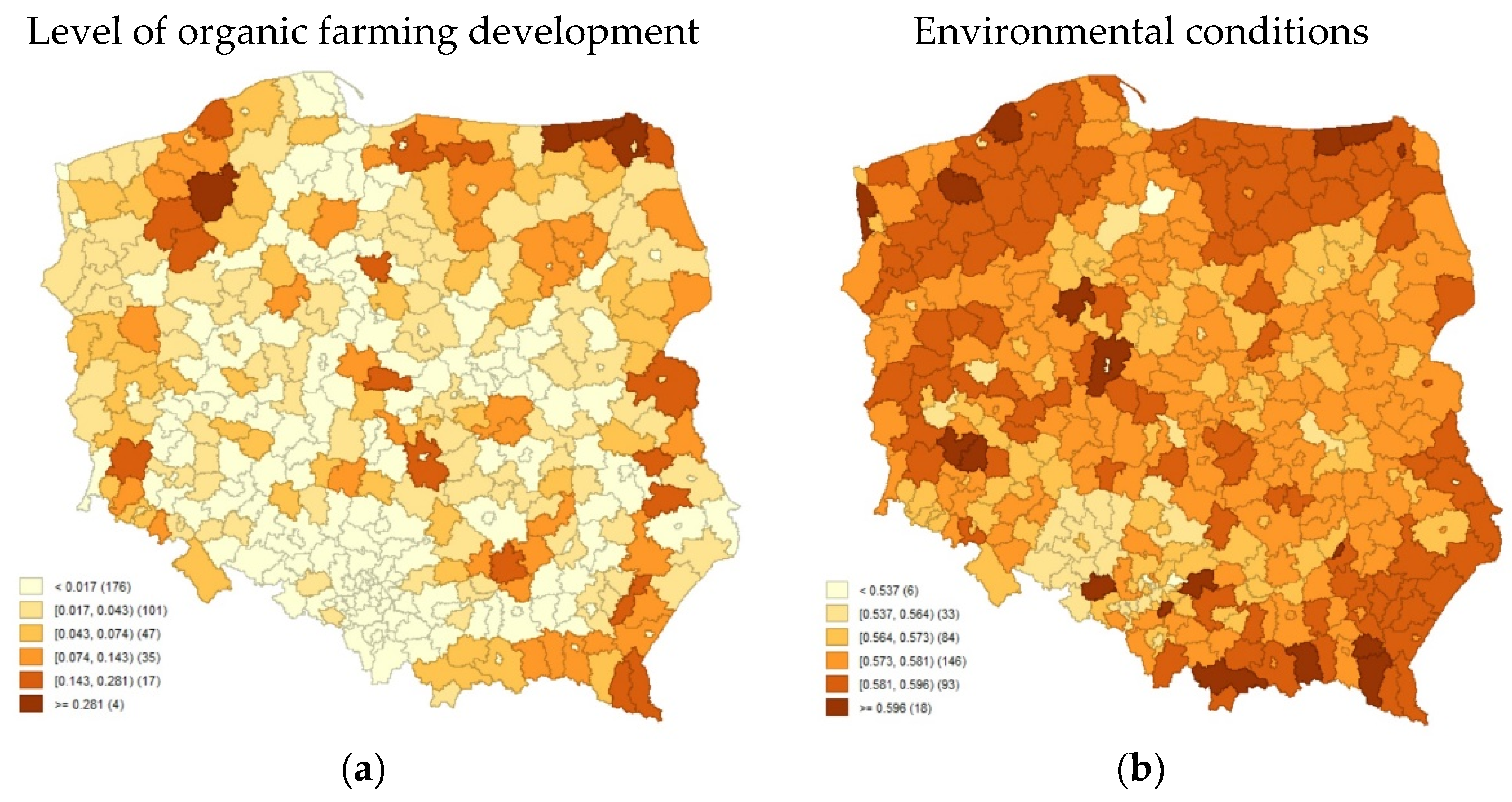
To visualise the obtained outcomes, the values of the synthetic measures are presented on a map below (
Figure 1).
The highest values of the synthetic measure concerning organic farming growth in the analysed objects were identified in the following districts: Szczecinecki (Zachodniopomorskie voivodship), Suwalski (Podlaskie voivodship), as well as Gołdapski (Warmińsko-Mazurskie voivodship). Within these regions, high (often the highest in Poland) variable values referring to the amount of organic farms, crop area and production of cereals, crop area of legumes for dry seeds, fodder plant production, and the number of cattle were observed. From the perspective of the growing demand for organic food, the values for these variables were favorable as they referred to the production of the important foodstuff and fodder used for further animal production. However, a significant weakness was a lack of variables referring to the fruit and vegetables characterized by a high consumer interest. Considering the environmental protection, the increase in the organic area for any crop and the amount of organic farms was vital.
Among 20 objects with the smallest values of the synthetic measure, 12 occurred in Śląskie voivodship, characterized by the highest degree of urbanization and population density in Poland, with the Upper Silesian Industrial District situated in the central part of the region (the most heavily industrialized area in Poland). In this region, very low values (often the lowest in Poland) of the particular partial variables were noted. This fact is not surprising since the state of the natural environment and contamination, especially of soil and water, makes it difficult to practice any agricultural activity, particularly organic farming, which should be applied in a clean environment so that the produced food does not absorb the harmful substances affecting food safety and quality.
Among 20 highest-rated districts taking into account environmental conditions, the highest values of the synthetic measure were noted in the following voivodships: Podkarpackie, Warmińsko-Mazurskie, and Zachodniopomorskie (three districts in each)—voivodships with relatively high forest cover and low population density. Among the objects with the smallest values of the constructed measure, high and very high values of partial variables relating to the dust pollution retained or neutralized in pollution abatement equipment as a percentage of generated pollution and industrial and municipal sewage treated as a percentage of sewage-requiring treatment, with relatively low values of the variables related to the consumption of fertilizers (fertilizers in total, phosphorus, and potassium) were observed. In turn, among the lowest-rated 20 districts considering the environmental conditions (with the lowest or very low values of the partial variables), every fourth district occurred in Śląskie voivodship (as earlier mentioned, the most heavily industrialized area in the country). It coincides with the lowest values for organic farming development, which confirms that it is impossible to practice organic agriculture in regions where the environment is contaminated. In these lowest-rated districts taking into account environmental conditions, the lowest values were observed in the case of the percentage of recovered waste, the total number of municipal and industrial wastewater treatment plants with increased removal of nutrients, and high values (which are not desirable considering the analyses performed) of the volume of municipal waste collected during the year, as well as indicators relating to fertilizer consumption were noted. These conditions significantly affect the state of the natural environment in the considered districts and reduce their attractiveness not only from the organic agriculture perspective but also their competitiveness, e.g., in terms of tourism, running a business in the various field of services or a good place to live at all, considering the influence of pollutants on human health.
Regarding the synthetic measure of organic farming development, right skewness was identified, which indicates that values were not higher than the arithmetic mean (classic coefficient of skewness amounted to 2.81). For 75% of districts, that measure did not exceed 0.0455 by the lowest value equal to 0. In the case of the synthetic measure of the environmental conditions, left-skewness of the distribution was identified (classic coefficient of skewness amounted to −1.15). For three of the considered districts, this measure was not higher than 0.582 (the lowest value amounted to 0.4925).
For such synthetic measures, a correlation analysis was conducted. For this purpose, the value of Spearman’s rank correlation coefficient among the synthetic measures of the considered multidimensional phenomena, constructed earlier based on the TOPSIS method, was determined. The correlation coefficient value was equal to 0.4142 and was statistically significant (p < 0.05). The strength of the correlation between the analysed occurrences should be considered average.
Then, canonical analysis was employed. As mentioned earlier, canonical correlation is a procedure that enables the assessment of the relations between two sets of variables. In this study, it was used to define the range and direction of the dependencies between sets of variables describing the level of organic agriculture development and selected environmental conditions. Due to the multifaceted nature of the analysed phenomena, the analysis of the dependence takes into account a large number of explained and explanatory variables.
Within the canonical analysis, the null hypothesis was the lack of connections between sets of variables, i.e., that all canonical correlations are equal to zero. If one may reject such a hypothesis, it is assumed that at least the first pair of the canonical roots that has the greatest values is statistically significant. The significance of the canonical roots was calculated using the Wilks lambda test, which is based on the principle of sequencing. First, all canonical variables were taken into account. In further steps, an attempt was made to reject the hypothesis about the lack of dependence of two sets of variables, disregarding the covariance mapped by the first k canonical correlations (
Table 4).
In the canonical analysis, the amount of generated canonical roots corresponds to a minimum amount of variables involved in one of the examined sets. In this case, it was 25 canonical roots, which resulted from the number of the reduced sets of variables explaining the environmental conditions. The first generated pair of the canonical roots, which synthetically described interactions between the considered sets of variables, explained most mutual relations. Hence, researchers mainly focus on the correlation for the first canonical pair. In turn, P. Churski [
67] claimed that from the variety of the estimated correlation coefficients, only the first with the highest value should be selected, referring to the maximum dependence between combinations of dependent and independent variables. Considering that the first pair of canonical roots does not entirely describe the relations between the analysed variables, it is essential to define the following pairs of canonical roots, which explain relations in other (less important) dimensions.
It is worth mentioning that generated canonical variables are mutually correlated (since they explain the dependencies between the sets of variables in different dimensions) and explain the lower and lower variability (similarly determined canonical correlations have lower and lower values). Nevertheless, according to the researchers, all the statistically significant canonical variables (in this case, two) should undergo analysis because they may reveal important information on the co-variability between the sets under consideration.
The determined canonical correlations were arranged in descending order of their values. The highest canonical correlation was equal to almost R = 0.75; the value of the Wilks lambda test checking the significance of the highest canonical correlation was 0.0531. A high and statistically significant value of the canonical correlation proves that the adopted linear model described the two sets of variables well. A low or statistically insignificant value of the canonical correlation did not provide grounds for interpreting the value of the canonical determination coefficient. The lack of correlation proves that the model was wrongly selected (the linear function should be changed) or that there was no real dependence between the analysed sets of variables. Apart from the two first canonical variables, the remaining determined pairs of canonical variables did not correlate with each other with statistical significance. Therefore—as mentioned earlier—they were omitted from further considerations.
It is worth mentioning that through the determination of the canonical roots, one may calculate 1-R2 values, which are estimators of the variance unexplained by successive canonical variables. These are so-called eigenvalues, which can be interpreted as a proportion variance explained by the correlation between the relevant canonical variables (this proportion is calculated in relation to the variance of canonical variables, i.e., weighted sums of two sets of variables). In this case, the eigenvalue for the first statistically significant canonical variable was equal to 0.5588 and for the second one—0.3652.
In the context of the conducted analyses, it is important to investigate the structure of dependencies between the analysed sets of variables. The determined canonical weights for both sets enable identification of the canonical variable structure by demonstrating the specific contribution of each variable to the weighted sum. These weights created for both standardized sets of variables are equivalents of beta coefficients in multiple regression.
Since the used variables underwent standardization, one may compare the absolute value of the generated canonical weights directly (
Table 5). Based on the performed calculations, one may conclude that concerning the first canonical root, the highest (absolute) weight values were calculated for variables OF19 (−0.8727) and E25 (1.1237). It may be assumed that the generation of the first canonical value was influenced by the area of pastures and meadows per capita and the consumption of potassium fertilizers per 1 ha. In turn, for the considered partial variables, OF1 (1.1497), describing the number of organic farms per capita and similarly as in the case of the first canonical root, variable E25 (−7.7911) mainly contributed to defining the second statistically significant canonical variable. It is worth mentioning that from the environmental point of view, both high values of the area of pastures and meadows and the number of organic farms are essential because any growth of the organic area, even of an extensive character, contributes to the improvement of the natural environment since the protected area is expanding.
Moreover, in order to learn about the structure of individual canonical elements, the canonical factor loadings were determined, reflecting correlation coefficients of a given canonical variable with output variables. The greater the value of the factor load (in absolute value), the more attention ought to be paid to this root when interpreting the canonical variable. The higher the value (in absolute value), the more emphasis ought to be put on this root when interpreting the data. T. Panek and J. Zwierzchowski [
68] recommend interpreting the roots in cases where the square of the correlation coefficient exceeds 0.50, whereas according to G. Więcek and A. Sękowski [
69], only those variables for which the value of the charges (and not their squares) is greater than 0.30 (in absolute value) should be analysed. For these analyses, the critical value of this correlation coefficient was also assumed at the level of 0.30.
Within the set of variables related to the environmental factors, in the case of the first canonical root, variable E18 had the highest factor loading (−0.9202), and for the second canonical variable, E14 (−0.4601). In the case of the set of variables explaining the level of organic farming growth, for the first canonical root, the highest factor loading was observed for the variable OF19 (−0.9194), and for the second, the variable OF7 (0.3736). There is sometimes an opinion among researchers that the canonical values of the canonical factor loadings should be used to interpret individual canonical variables [
68]. The argument is that they can be intuitively understood. Nevertheless, one ought to remember that the values of those measures describe the correlations of specific primary variables with canonical roots. In contrast to canonical weights, they do not take into account covariate impacts for a certain set of primary variables; interpreting canonical roots involving the values of correlation coefficients might result in diverse conclusions than a comprehensive multidimensional analysis involving canonical weights [
68]. This approach was used for this study.
Considering the canonical weights and factor loadings, one may conclude that the first statistically significant canonical variable described the relations as follows:
The greater the share of renewable energy relative to the total electricity production (E26), the greater the number (per capita) of farms (OF1) and the greater the area of crops: cereals (OF3), legumes for dry seeds (OF5), crops of potatoes (OF7), and beet crops and root crops (OF9). This may, to some extent, indicate increased environmental responsibility of economic entities (including organic farmers). Generally, in regions where organic farming is performed, other environmentally friendly actions are undertaken since the level of environmental awareness is relatively high. Further, organic farmers are willing to undertake this type of activity such as relative to production and use of renewable energy, which is in line with the results of Smith et al. [
6].
The greater the share of renewable energy relative to the total electricity production (E26), the greater the production (per capita) of cereals (OF4), potatoes (OF8), and forage plants (OF18), which also confirms the positive correlation between various environmentally friendly activities. This proves that organic farmers apply environmental principles as a whole and not on a selective basis relating to their pro-environmental activity to, e.g., financial incentives.
For the production of cereals (OF4), potatoes (OF8), and forage crops (OF18) and the cultivation area of cereals (OF3), legume crops for dry seeds (OF5), potatoes (OF7), and beetroot and root crops (OF9) positively impacted the saturation of individual areas with municipal wastewater treatment plants with increased removal of nutrients per 1000 inhabitants (E18) and the share of legally protected areas relative to the total area (E6). This may prove that the level of water contamination may influence the level of production of particular crops. Apart from that, the share of legally protected areas has a significant meaning. It contributes to the overall improvement of the natural environment state in the protected area or even extends this for the whole region.
The share of legally protected areas relative to the total area (E6) had a positive effect on the number of sheep (OF20) and cattle (OF22). This may mean that the greater the legally protected areas, the better the conditions for organic farming methods, especially for the more extensive types of production such as livestock, in this case, sheep and cattle, which require large areas of clean pastures.
While analysing the factor loading values and canonical weighs for the second statistically significant canonical variable, one can conclude that a positive dependence between the share of legally protected areas relative to the total area (E6), dust pollution retained or neutralized in pollution abatement devices relative to the percentage of pollution produced (E10), and the area and potato production (OF7 and OF8) occurred. It is worth mentioning here that the forms of environmental protection are, among others, national parks. There are 23 national parks in Poland. The Podlaskie Voivodship is characterised by the largest area of national parks (more than 92 thousand ha); Podkarpackie Voivodship is second (more than 47 thousand ha) and is followed by Mazowieckie Voivodship (more than 38 thousand ha). The smallest area of national parks is, in turn, in Wielkopolskie (nearly 8 thousand ha), Świętokrzyskie (7.6 thousand ha), and Łódzkie (68 ha) voivodships. It can also be assumed that with the decrease in the volume of municipal waste collected during the year (E2) and the percentage of waste recovered, the area of industrial crops (OF11) decreases. Again, the influence of the legally protected areas on the organic area and the production of organic food has been confirmed, and they may be perceived as among the most important environmental, positively correlated, factors of organic farming development.
It is assumed that the correlation square called the coefficient of determination reflects the share of the variance of one variable described by another variable. If we square the values of the factor loadings representing the correlation, we get the proportion of the variance of a certain variable described by the canonical root. When we calculate the average of these proportions for all variables for a given canonical variable, we will obtain information on the share of the variance described by the average certain canonical root in the data set. This variance is called the extracted variance (see
Table 6).
In turn, the eigenvalues of the matrix related to the correlation matrix of the variables of both sets multiplied by the square of the canonical correlation yield a new synthetic index called the redundancy of a given set of variables for the second set. This value indicates what part of the average variance within the first set is described by a certain canonical root when the second set is known. In other words, we learn to what extent the redundancy of a given canonical variable tells us how much of the average variance in one set is explained by a given canonical variable when we know the second set. Thus, we find out how redundant one data set is for a given second data set. Total redundancy is the sum of the redundancy of all canonical variables.
The most statistically significant canonical root distinguished nearly 7% of the variance in the set of variables relating to the environmental factors and almost 18% in the second set (describing level of organic agriculture growth). On the other hand, the second canonical root distinguished about 3.5% of the variance in both sets. For the set of variables referring to the level of organic farming growth, one may explain 10.05% and 1.3% of the variance of the variables describing the environmental factors. In turn, for the set of primary variables related to the environmental factors, 3.68% and 1.28% of the variance was described using the first two statistically significant canonical variables. Thus, the second canonical root had a minor contribution to the description of this variability.
In the subsequent step, the value of whole redundancy was estimated, which is understood as the mean share of the variance described in the first set of variables relative to a second set, involving all canonical roots. The performed estimations demonstrated that knowing the values of the variables explaining the environmental conditions, one may clarify nearly 26.70% of the variance of the variables within the set describing the level of organic farming development. This value can be evaluated as moderate. Therefore, further research with a different set of primary variables should be performed.
When analysing multidimensional relations between environmental conditions and the level of organic farming development, it is worth noticing high and highly statistically significant canonical correlation values (see
Table 4. However, one should remember that the canonical correlation may not be interpreted identically as a classic correlation (e.g., Pearson’s). These correlations occurred between weighted sum values in every set with weights estimated for the successive canonical roots. The value of the highest and most statistically significant canonical correlation amounted to almost 0.75, and for the second statistically significant canonical root, this value exceeded 0.60. The square of these canonical correlations estimates the degree of explanation through linear dependencies of the variability of the first set of variables, through another input set, by successive pairs of canonical roots. Considering the first statistically significant canonical root, the square of the canonical correlation exceeded 0.56, whereas for the second one, nearly 0.37. One may assume that the constructed model explains the analysed data sets relatively well.
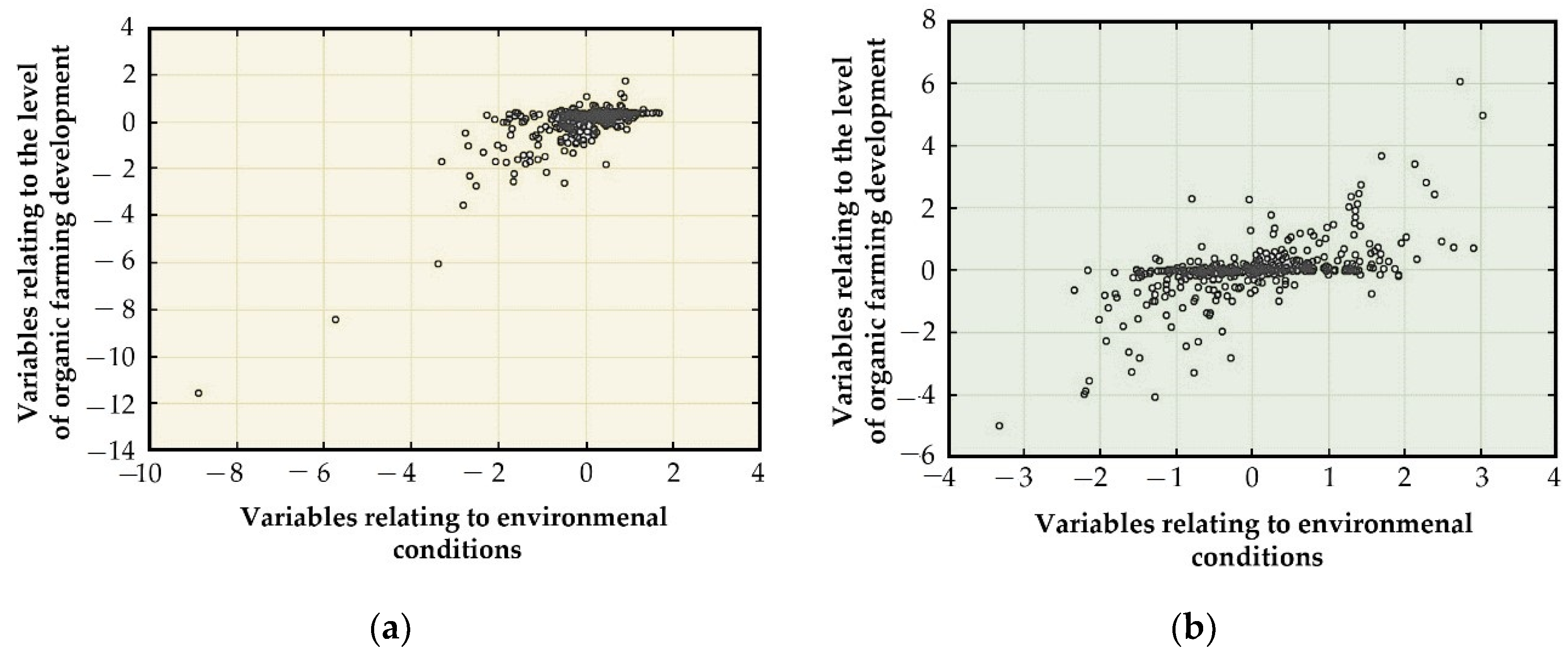
Figure 2 presents scatter plots of the first and second statistically significant canonical root. It shows the relations between the values of the newly created variables relating to environmental conditions (OX axis) and the level of organic farming growth (OY axis).
For the first statistically significant canonical root (
Figure 2a), no strong scattering of points demonstrating the considered objects was noted (districts in Poland). These points were arranged along a straight line (with a positive slope). This proves that these generated pairs of canonical roots carried a significant part of the information about the covariance of the two considered sets of input variables. One may assume that together with the growth in values for the groups of causes, the values of results increased in total, and this relationship was clearly linear, as shown in the figure above. The proximity of most of the points (in the case of canonical analysis, representing the considered districts) may indicate a similar structure of the input variables. In the scatter plot prepared for the second statistically significant canonical variable, points representing analysed objects were also arranged along the positively sloped straight line, but they were more scattered (
Figure 2b). Such an arrangement of points means that the second pair of canonical roots carried less information about the covariate of the considered variables than the first pair of canonical roots.
5. Conclusions
The state of the natural environment impacts the quality of agricultural products that may be a source of various types of threats, both of biological and chemical character. Guaranteeing the health safety of food is particularly important in the case of organically produced food, where the use of chemical protection agents in the production of raw materials, reducing the risk of biological hazards, is not allowed. Organic production requires good environmental conditions so that organic products cannot absorb soil, water, or air substances that are harmful. Therefore, it is essential to recognize the significant environmental factors and determine their influence on the level of organic farming development, taking into account the spatial distribution and intensity of variables related to both environmental determinants and organic farming development.
Thus, the objective of the conducted research was to recognise the relations between the level of organic farming development and chosen environmental conditions in Poland. Thanks to the multifaceted character of both phenomena considered, it seemed advisable to use canonical analysis. In the context of studying complex economic phenomena, the popularization of the use of multifaceted exploratory methods (e.g., canonical correlation) is of particular importance.
Considering the TOPSIS outcomes, the districts with a relatively high level of organic farming development were generally also described by a relatively high level of the selected environmental determinants for organic agriculture development. However, the performed empirical analyses proved that environmental factors were important but not the only determinants of organic farming development (one may also distinguish financial, institutional, or market factors). Based on the conducted correlation analysis, it can be concluded that between synthetic measures of the investigated phenomena, constructed using the TOPSIS, there was positive, moderate, and statistically significant dependence (the determined Spearman’s rank correlation coefficient exceeded 0.41). The classic coefficient of variation for the constructed measure of the level of organic farming development exceeded 140%, while the standard deviation exceeded 0.05 (mean value close to 0.04). This confirms the significant diversification of the level of organic farming development in Poland (measured at the district level). On the other hand, the coefficient of variation for the environmental conditions was less than 2.5% for the constructed synthetic measure of environmental conditions, which can be interpreted as a relatively weak differentiation for the analysed occurrence (for the variables included in the research). Therefore, there is a need for further research, including in the model other factors determining the development of organic agriculture, e.g., market factors, to explain the complexity of the phenomenon more completely. Market factors may play an important role in organic farming development since they influence the profitability of agricultural activity. Nevertheless, this study would require performing a survey on farmers to explore the impact of such factors as sales volume, marketability of farms, prices for farm products, distance to larger markets (cities), etc. Further, including in the future study other factors of environmental character, relating to agricultural conditions, such as topography, soil, water, or climate conditions, would be valuable as well. However, their involvement depends on data availability.
As part of the canonical correlation, two statistically significant canonical roots were determined. Taking into account the redundancy coefficient value calculated as part of the canonical analysis, one can state, knowing the values of the variables describing the environmental conditions, nearly 26.70% of the variance of the variables from the set describing the level of organic agriculture development was described. This means that more than one quarter of the variability related to the level of organic farming (for the partial variables included in the analysis) was estimated by the variables related to environmental conditions. It is worth mentioning that high values of canonical correlation coefficients were identified for statistically significant canonical roots. Concerning the most statistically significant canonical root, the coefficient was 0.75, and in the case of the second statistically significant canonical root, the value slightly exceeded 0.60. Based on the squares of the canonical correlations, it can be assumed that the constructed models described the analysed data sets relatively well.
The conducted research proved that environmental conditions have meaning for organic agriculture development. The research showed a positive dependence between the share of renewable energy produced in the districts and the area and the production of certain agricultural products such as cereals, potatoes, beet and root crops, and forage plants, which are among the most important organic products. This means that generally, environmentally friendly practices go together. This may result from the fact that organic farmers are often pioneers and leaders in the local community. They may implement innovative, environmentally friendly solutions in their farms, e.g., installing photovoltaic panels, and others follow their actions. For the same reason, the level of environmental awareness (raised by the community leaders) may be relatively higher. Therefore, it is vital to support environmentally friendly practices in rural areas to enhance their total impact by a synergistic effect.
The research also demonstrated that from various environmental conditions, the high share of the legally protected areas influenced the crop area and the production of particular organic agricultural foodstuff. This has meaning in both types of production of more (such as sheep and cattle) and fewer (potatoes, cereals beetroots, fodder) extensive characters. The influence of the share of protected areas is particularly important in the case of organic animal production, which is insufficient in Poland. Therefore, the growth of the protected areas might contribute to balancing the supply with the growing market demand for organic meat. It is obvious that the measures to protect the environmentally valuable regions also favour organic farming, which can be performed under the best possible conditions. Therefore, it is vital for policymakers to increase the area of national and landscape parks and, on the other hand, to encourage farmers in these areas to undertake organic farming since their produce originating from the least contaminated environment is of the highest quality.
Furthermore, the study showed that the most polluted regions were characterised by a very low level of organic agriculture growth. On the other hand, the least polluted areas were also distinguished by a high level of organic farming development. Apart from renewable energy use and the share of protected areas, factors such as fertilizer consumption, collected and recovered waste, and wastewater treatment, have meaning for organic farming development as well in the discussed districts. Therefore, measures aimed at more effective waste and wastewater management should be taken into account by policymakers while designing the assumptions for measures aimed at improving the situation of the most polluted regions. They should consider introducing more effective regulations and actions to reduce pollution and restore the already damaged areas. To summarize, they ought to focus in particular on the activities to expand the protected areas and improve recovery of waste and water, reduce generated waste, and generally better manage both fields. Implementation of measures aiming to recover the natural environmental state would not only contribute to the development of organic agriculture but also raise the attractiveness and competitiveness of these regions. On the other hand, improving conditions for organic farming development should be particularly taken into account. Due to frequently occurring food allergies and relatively high consumer incomes in industrialized regions, the demand for organic food is quite high. Therefore, the development of organic agriculture in these regions could contribute to the reduction of transaction costs and the unfavourable impact of transportation of organic products on the natural environment.
We realise that there are limitations of the present study. The most significant was the availability of the data, particularly originating from the Main Statistical Office in Poland, which generally provides information for the larger administrative unit—voivodships and only selected ones were available at a district level. Therefore, some variables selected on a substantial basis had to be rejected due to the lack of availability. In further research, it will be worth carrying out dynamic research (over a certain period). In addition, it is worth trying to use a system of weights for the variables used to differentiate their rank. Analyses concerning smaller spatial units and between certain territorial units would be valuable, but a significant problem is the smaller range of potential diagnostic variables available at this level. The authors are also aware that the use of secondary data in this article is associated with specific outdated information, and to some extent with their general nature, therefore it is worth carrying out similar research using questionnaires in the future.


