CFD Study on the Ventilation Effectiveness in a Public Toilet under Three Ventilation Methods

Abstract

The indoor air quality (IAQ) of severely polluted toilets is associated with the transmission of diseases. Computational fluid dynamics (CFD) methods and experimental measurements were used to analyze the diffusion characteristics of pollutants. This study investigated the diffusion characteristics and normalized concentration of ammonia and hydrogen sulfide pollutants under three ventilation systems—mixing ventilation (MV), personalized ventilation (PV), and impinging jet ventilation (IJV)—in a public toilet. The mean age of air (MAA) and air exchange efficiency (AEE) were also analyzed in our study. The results show that the MV scheme has a poor removal effect on pollutants compared with PV and IJV. IJV has advantages in reducing the normalized concentration of pollutants and improving the IAQ. Increasing the number of air changes per hour (ACH) may lead to a longer MAA and reduced air exchange efficiency. Choosing an appropriate number of air changes is very important to improve the IAQ in the toilet.

1. Introduction

Indoor air pollution is harmful to human health [1,2], causing issues such as respiratory infections, asthma, and lung cancer [3,4,5]. We spend more than 90% of our time indoors [6]. Hence, indoor air quality (IAQ) is vital to our well-being [7]. People are now paying much attention to the IAQ [8]. The toilet is frequently used, and it emits many undesirable odors such as ammonia and hydrogen sulfide [9,10]. The maximum ammonia and hydrogen sulfide concentration in first-class public toilets should be 0.3 mg·m⁻³ and 0.01 mg·m⁻³, respectively [11]. It is essential to remove pollutants quickly and provide sufficient fresh air to achieve suitable IAQ [12,13,14]. Natural ventilation is an energy-efficient way to improve the IAQ, but it often cannot meet the ventilation needs.

There is little literature on toilet ventilation, including the overall ventilation performance of the toilet, the efficiency of toilet components, and IAQ measurements [15]. Tung et al. [16,17,18] constructed experimental modeling of foul-odor diffusion from the toilet, and the conclusion is that the forced ceiling-supply and wall-exhaust systems show the best ventilation performance. Tung et al. [17] analyzed the effects of the ACH on the distribution of the pollutant concentration. Chung et al. [19] analyzed the influence of the number of windows on the distribution of air pollutants in a public toilet. The results show that a sufficient number of sunshade windows and suitable installation positions help to achieve the best ventilation effect.

Computational fluid dynamics (CFD) was widely used in air distribution [20,21,22,23], pollutant diffusion [24,25,26], and particle transportation [27]. Cao et al. [28] stated that the MV system aims to produce low-pollution-concentration air for the room; however, the fresh air in breathing zones is less than 1%. Wang et al. [29] compared the difference in air particles between MV and IJV, indicating that the IJV has high efficiency in removing pollutants. For mixed ventilation, the location of the pollutant source has a negligible effect on the diffusion of pollutants in the respiratory zone [30].

The concept of personalized air was presented in 1999 [31]. Personalized ventilation (PV) supplies fresh air directly to the occupant’s breathing zone [32]. As an efficient ventilation method, PV has attracted increasing attention [33]. Melikov and Cermak [3,34] found that PV could reduce the concentration of pollutants, and could significantly improve the thermal comfort [35,36]. However, it may affect the transmission of pollutants in some unfavorable combinations [37,38].

The IJV system recommended in the late 1990s was considered a new method of ventilation [20]. IJV has attracted much attention owing to its advantages in energy saving and being suitable for heating and cooling modes [39]; it has a better mean MAA and velocity field due to the better balance between buoyancy and momentum [40,41]. The IJV system improved the air quality in the breathing zone and consumed less energy than the MV system in heating mode [42,43], and researchers have been working on optimizing its performance in HVAC systems [44,45]. The IJV system has a lower airflow rate than the MV and DV systems in cooling mode [46].

Karimipanah et al. [20,40] focused on the performance of IJV and DV systems and found that the IJV system has a higher ventilation effectiveness and produces better velocity distribution in the occupants’ zone. Yao et al. [47] studied the flow characteristics of the isothermal impinging jet in a closed cabin using experimental methods and discussed the multi-purpose characteristics of the jet impinging structure. Research to investigate the shape of the appropriate supply device has been carried out. Cooper et al. [48] investigated the flow field of a three-dimensional turbulent impinging jet using experimental methods and then discussed the attenuation of the axial velocity and rate of jet growth.

The local mean MAA characterizes the time needed for air to move from the inlet to a particular location in the indoor space [49,50,51,52]. Buratti and Palladino [53] studied the influence of window airtightness and environmental conditions on MAA and the application of artificial neural networks in the prediction of indoor CO₂. They found that airtightness and indoor and outdoor air temperature have a great influence on the air quality of naturally ventilated buildings. The artificial neural network is reliable in predicting the concentration of CO₂ in the room and can be used to assess the age of the indoor air. Mao et al. [54] concluded that the lower MAA is a good indicator of the well-ventilated zones. The local MAA is a better and more sensitive parameter than the average air velocity. It is used to highlight areas with insufficient ventilation to evaluate the ventilation efficiency of industrial food factories [55]. Ng et al. [56] discussed the advantages of the monotonic resolution scheme in the study of indoor airflow; the results show that the accuracy of the scheme was very high, and the simulation results were in good agreement with the measured results. The air exchange efficiency (AEE) was used to characterize indoor airflow patterns and analyze their ventilation performance [18,57].

At present, many studies have focused on the natural or mechanical ventilation of buildings. Scholars have seldom studied the distribution of pollutants in public toilets, especially the application of MV, PV, and IJV in toilet ventilation. The evaluation of IAQ and ventilation efficiency of public toilets is not perfect. The present study investigated pollutant diffusion using numerical simulations and experimental methods.

2. Methods

2.1. Physical Model

A public toilet in Zhejiang (China) was chosen as the research model (see Figure 1). A test chamber was used to verify the numerical model, as shown in Figure S1 in Supplementary materials. The geometric data of the investigated model are shown in

Table 1. Geometric data.

Parts of the Model	Geometric Data (m)
Public toilet	7.8 × 4.3 × 2.6
Test chamber	0.96 × 0.96 × 2.2
Pollution source	0.5 × 0.2
M1	(X) 0.2 × (Y) 0.2
M2	(Y) 0.4 × (Z) 0.4
U1	(X) 0.2 × (Z) 0.2
S1	(X) 0.2 × (Z) 0.2
S3	(X) 0.2 × (Z) 0.2
J1	(X) 0.2 × (Y) 0.2
J6, J7	(Y) 0.3 × (Z) 0.06
Urinal	r = 0.1
Stall	(X) 0.2 × (Y) 0.3
Window-1	(X) 0.965 × (Z) 0.6
Window-2	(Y) 0.55 × (Z) 1.4
Door	(Y) 1.2 × (Z) 2.1

.

Table 2. Case description.

Case	Exhaust Fan Position	ACH (h−1)
MV-1	M1	5, 10, 15, 20, 25, 30
MV-2	M2	5, 10, 15, 20, 25, 30
PV-1	U1, S1	2.5, 5, 7.5, 10, 12.5, 15
PV-2	U1, S2	2.5, 5, 7.5, 10, 12.5, 15
PV-3	U1, S3	2.5, 5, 7.5, 10, 12.5, 15
IJV-1	U1, J1	2.5, 5, 7.5, 10, 12.5, 15
IJV-2	U1, J1	2.5, 5, 7.5, 10, 12.5, 15
IJV-3	J1	5, 10, 15, 20, 25, 30
IJV-4	J2	5, 10, 15, 20, 25, 30
IJV-5	J3	5, 10, 15, 20, 25, 30
IJV-6	J6	5, 10, 15, 20, 25, 30
IJV-7	J7	5, 10, 15, 20, 25, 30

lists the ACH in each case.

2.2. Experimental Setup

SF₆ is often used as a tracer gas in experiments [58]. It flows out from the gas cylinder into the test chamber (see Figure S1). The release rate was 60 mL/min.

An XLA-BX-SF₆ instrument with an error of ±0.01 ppm was used to measure the gas concentration. Each measurement time was 45 min, and data were recorded every 30 s.

2.3. CFD Setup

2.3.1. Numerical Method

The standard k–ε, RNG k–ε, realizable k–ε, and low-Re k–ε models were used to simulate the gas turbulence [59]. The CFD model was constructed according to the conditions applied in the experiments (see Figure S1); an unstructured computational grid of polygon elements with a mesh number of 1.09 million (when it increases to 1.65 million, the maximum difference between the two results is 3%) (Figure S2a).

Governing equations are as follows:

$$\frac{\partial \rho }{\partial t}+\frac{\partial \left(\rho u\right)}{\partial x}+\frac{\partial \left(\rho v\right)}{\partial y}+\frac{\partial \left(\rho w\right)}{\partial z}=0,$$

(1)

Turbulence equation:

$$\frac{\partial \left(\rho K\right)}{\partial \tau }+\frac{\partial \left(\rho K{u}_i\right)}{\partial X_i}=\frac{\partial }{\partial X_i}\left[\left(\mu +\frac{u_t}{{\sigma }_K}\right)\frac{\partial K}{\partial X_j}\right]+G_K+G_b-\rho ϵ$$

(2)

Species transport equation:

$$\frac{\partial \left(\rho u{c}_s\right)}{\partial x}+\frac{\partial \left(\rho v{c}_s\right)}{\partial y}+\frac{\partial \left(\rho w{c}_s\right)}{\partial z}=\frac{\partial }{\partial x}(\frac{D_s\partial \left(\rho c_s\right)}{\partial x})+\frac{\partial }{\partial y}(\frac{D_s\partial \left(\rho c_s\right)}{\partial y})+\frac{\partial }{\partial z}(\frac{D_s\partial \left(\rho c_s\right)}{\partial z})$$

(3)

Momentum equation:

$$\frac{\partial \left(\rho u\right)}{\partial t}+div\left(\rho uV\right)=-\frac{\partial p}{\partial x}+\frac{\partial {\tau }_{xx}}{\partial x}+\frac{\partial {\tau }_{yx}}{\partial y}+\frac{\partial {\tau }_{zx}}{\partial z}+F_X$$

(4)

$$\frac{\partial \left(\rho v\right)}{\partial t}+div\left(\rho vV\right)=-\frac{\partial p}{\partial x}+\frac{\partial {\tau }_{xx}}{\partial x}+\frac{\partial {\tau }_{yx}}{\partial y}+\frac{\partial {\tau }_{zy}}{\partial z}+F_Y$$

(5)

$$\frac{\partial \left(\rho \omega \right)}{\partial t}+div\left(\rho \omega V\right)=-\frac{\partial p}{\partial x}+\frac{\partial {\tau }_{xz}}{\partial x}+\frac{\partial {\tau }_{yz}}{\partial y}+\frac{\partial {\tau }_{zz}}{\partial z}+F_Z$$

(6)

Energy equation:

$$\frac{\partial \left(\rho T\right)}{\partial t}+div\left(\rho \overline{u}T\right)=div\left(\frac{k}{c_p}gradT\right)+S_T$$

(7)

where ρ is the air density; t is the time; u, v, and w are the velocity components in the x, y, and z directions; τ is the time; K is the turbulent kinetic energy; C_S is the volume concentration of the component s; and D_S is the diffusion coefficient of the component s.

2.3.2. Boundary Conditions

The exhaust outlet and windows were set as the velocity outlet and pressure outlet, respectively [10,60]. He ammonia release concentration was 2.5 × 10⁻⁷ kg/s and hydrogen sulfide release concentration was 6 × 10⁻⁸ kg/s.

An unstructured computational grid was applied (Figure S3). Different numbers of grids were divided for grid verification, which were 1,028,048, 1,498,338, 2,346,227, and 3,343,910, respectively. When the mesh number was greater than 2,346,227, the pollutant concentration and flow rate changed little, and the maximum difference between the two results was 7%, 9%, and 5%; we chose this for our study (Figure S4).

2.4. Evaluation Index

The normalized concentration of the pollutant was selected for the analysis [61].

$$\epsilon =\frac{C}{{{\displaystyle c}}_{NV}}$$

(8)

where C_NV and C are the average pollutant concentration under natural ventilation and mechanical ventilation, respectively.

The local mean $\overline{{{\displaystyle \tau }}_{\mathrm{s}}}$ age of air (MAA) is calculated by the following equation:

$$\overline{{{\displaystyle \tau }}_{\mathrm{s}}}={\displaystyle \underset{0}{\overset{\infty }{\int }}\frac{{{\displaystyle 60C}}_{\mathrm{s}}(t)dt}{{{\displaystyle C}}_0}},$$

(9)

where C_s(t) stands for the pollutant concentration at the monitoring surface Z = 1.5 m at time t, and C₀ is the concentration of the pollution source within the toilet. This study developed a user-defined function (UDF) in ANSYS Fluent to solve for MAA [49].

The room mean MAA was $\overline{{{\displaystyle \tau }}_r}$ used to calculate the AEE of the toilet and is calculated by the following equation [57]:

$$\overline{{{\displaystyle \tau }}_r}=\frac{{\displaystyle \underset{0}{\overset{\infty }{\int }}{{\displaystyle t\cdot C}}_{\mathrm{e}}(t)dt}}{{\displaystyle \underset{0}{\overset{\infty }{\int }}{{\displaystyle C}}_{\mathrm{e}}(t)dt}},$$

(10)

where t refers to the decay period, s, and C_e(t) is the concentration of the tracer gas in the exhaust air at time t, mg/m³.

To evaluate the ventilation performance of the toilet, AEE is calculated by the following equation [62]:

$$\mathrm{AEE}=\frac{{{\displaystyle \tau }}_{\mathrm{n}}}{2\overline{{{\displaystyle \tau }}_r}}\times 100\%$$

(11)

where ${{\displaystyle \tau }}_{\mathrm{n}}$ and $\overline{{{\displaystyle \tau }}_r}$ indicate the nominal time constant, min., and the MAA, respectively. The nominal time constant is defined as the ratio of the interior volume of the toilet (V), m³, to the volumetric outdoor airflow rate entering the toilet (Q), m³/s.

2.5. Validation of the CFD Simulation Method

The experiment was carried out in the school laboratory of Tongji University. The test chamber was fully ventilated before starting the experiment to prevent the residual SF6 gas in the test chamber from affecting the experimental results (Figure S1).

The CFD simulation results and the experimental data under the same conditions are compared, as shown in Figure S2b. The results of the standard k-ε model are reasonable, revealing the largest and smallest differences of 10% and 4%, respectively. The standard k-ε model has been widely used, and the difference between simulated data and experimental data is small. This model can be used to predict the distribution of indoor pollutants [21,61].

3. Results and Discussion

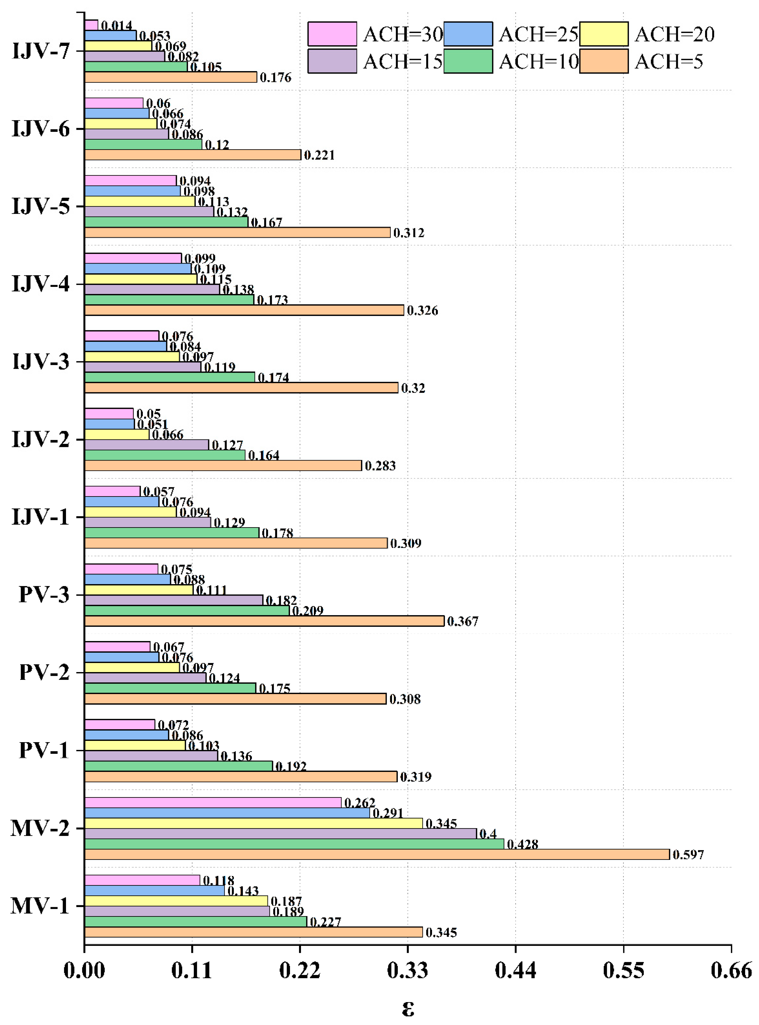
3.1. Performance of MV, PV, and IJV with Ammonia in the Occupied Zone

The ACH should be greater than 5 h⁻¹ [11] and 10–15 h⁻¹ in toilets [63]. This article chose 5, 10, 15, 20, 25, and 30 h⁻¹ (Table 2). The normalized ammonia concentration value of the Z = 1.5 m cross-section is shown in Figure 2. The normalized ammonia concentration value gradually decreases with the increase in the ACH. When the ACH is 5, the normalized concentration value achieves the maximum and minimum values in M V-2 and IJV-7, which are 0.597 and 0.176, respectively. The normalized concentration values of IJV-2 and IJV-6 are 0.283 and 0.221, respectively; the normalized concentration values of other schemes are greater than 0.3. The ammonia concentration and velocity cloud diagrams of the Z = 1.5 m section are shown in Figure 3 and Figure 4, respectively. The ammonia concentration directly above the urinal and in the toilet stall of MV-2 is high, and the ammonia concentration near the door hole and the exhaust fan is low (Figure 3b); the gas velocity near the exhaust fan is large and streamlined. It is denser than other areas in the toilet, and the flow lines in the toilet stalls become sparse due to the obstruction of the baffle (Figure 4b).

IJV-7 has a low ammonia pollutant concentration, high pollutant concentration in a small area in the toilet stall, and very low pollutant concentration at the toilet door (Figure 3l); this program has a low vent position inside the toilet stall. The gas velocity is small, and the flow lines are sparse. The flow lines in other areas of the toilet are dense. Near the doorway, the flow velocity is very high (Figure 4l). IJV-6 and IJV-7 use the same ventilation method, but the positions of the vents are different. IJV-6 has a higher normalized concentration value than the IJV-7, and the pollutant concentration in the stall closest to the vent is higher (Figure 3k); the wall directly opposite the vent has a high flow velocity, dense flow lines, dense flow lines near the urinal, and high wind speed (Figure 4k). The concentration of pollutants at the entrance of the IJV-2 is lower than that in other areas. Natural ventilation enters the toilet through the door opening, and the pollutants are easily diffused. The area of high concentration area is small (Figure 3g), and the airflow in the toilet stall is dense, the wind speed is high in the area near the wall, and the vortex is formed in the toilet stall, which may hinder the diffusion of pollutants (Figure 4g).

MV-1 has a normalized concentration value of 0.345, the distance between the urinal and the air outlet is long, and the baffle between the stalls obstructs the flow of gas, so the concentration of pollutants directly above the urinal and the stalls is very high, and the concentration of pollutants in the other positions is low (Figure 3a), whilst the air velocity directly above the toilet is high. Due to the obstruction of the baffle, a vortex is formed in the toilet. Natural ventilation enters the toilet from the door hole. The flow lines near the door hole are dense and have a high wind speed (Figure 4a).

The normalized concentration values of PV-1, PV-2, and PV-3 are 0.319, 0.308, and 0.367, respectively. The air supply positions near the urinals of the three schemes are the same, the air supply positions between the stalls are different, and the air supply position is in the stall. When the door opening is located (PV-2), a better ventilation effect can be obtained. In the PV-1 program, the concentration in the toilet stall and the vicinity of the two urinals are high, and in the rest area is very low (Figure 3c), and the wind speed at the baffle of the toilet in the middle of the toilet is high (Figure 4c); the PV-2 scheme has high concentration near the baffle in the toilet stall and near a urinal, low pollutant concentration in other areas (Figure 3d), and high flow velocity near the air outlet (Figure 4d); the PV-3 program has a high pollutant concentration near the doorway (Figure 3e), the wind speed near the doorway is high, and the wind speed in the rest of the area is low. The position of the air outlet of this program is relatively low, and the airflow velocity of the air outlet has little effect on the monitoring surface speed (Figure 4e).

The normalized concentration value of IJV-1 is higher than IJV-2, which is 0.309. The two programs use the same ventilation method near the stall. IJV-1 provides air near the urinal, the concentration of pollutants in some areas near the urinal is relatively high, and the air supply has a weak ability to take away pollutants (Figure 3f). The flow lines in the middle of the toilet are relatively dense and have a high wind speed (Figure 4f). The normalized concentration values of IJV-3, IJV-4, and IJV-5 are 0.32, 0.326, and 0.312, respectively. The height of the air outlet of the three schemes is different. The pollutant concentration distribution law of the monitoring surface (Z = 1.5 m) is different (Figure 3h–j); the three schemes form a vortex in the toilet stall, the airflow velocity is high, and the streamlines are dense; in the rest of the area, the streamlines are sparse, and the speed is relatively low (Figure 4h–j). IJV-5 is close to the monitoring surface, so the wind speed is high.

When ACH is 10, the normalized concentration value achieves the maximum and minimum values in the schemes MV-2 and IJV-7, which are 0.428 and 0.105, respectively. The normalized concentration values of MV-1 and PV-3 are 0.227 and 0.209, respectively, and the normalized concentration values of the other schemes are less than 0.2. When the ACH increases from 5 to 10, the normalized concentration values of the twelve schemes are, respectively, reduced by 0.118 (MV-1), 0.169 (MV-2), 0.127 (PV-1), 0.133 (PV-2), 0.158 (PV-3), 0.131 (IJV-1), 0.119 (IJV-2), 0.146 (IJV-3), 0.153 (IJV-4), 0.145 (IJV-5), 0.101 (IJV-6), and 0.071 (IJV-7). The normalized concentration of IJV-7 drops by less than 0.1, and the drops in the normalized concentration values of the other schemes all exceed 0.1. The normalized concentration values of different schemes are affected differently by the number of air changes; increasing the number of air changes can effectively remove ammonia pollutants.

When the ACH is 15, the normalized concentration value achieves the maximum and minimum values in the schemes MV-2 and IJV-7, which are 0.4 and 0.082, respectively. The normalized concentration value of IJV-6 is 0.086, and the normalized concentration value of the other schemes is greater than 0.1. In the MV-2 program, the concentration of ammonia gas in the toilet stalls is very high, especially in the stall near the doorway (Figure 5b). The wind speed in the toilet stalls is low. Wind speed in the toilet is low and the ammonia emission is not smooth. The flow lines near the exhaust fan are dense, and the flow velocity is high (Figure 6b). In the IJV-7 scheme, there is a high ammonia concentration in the toilet stalls and a very low ammonia concentration in the rest of the area (Figure 5l). The wind speed in the area near the doorway is relatively high, which accelerates the diffusion of pollutants (Figure 6l). The normalized concentration values of IJV-6 and IJV-7 are shallow, so the IJV-6 program has a good pollutant removal effect, and the pollutant concentration is deficient (Figure 5k). The wind speed near the window is high, which is good for pollutants. Exhaust through the window is shown in Figure 6k. In the other schemes, the high concentration area of the pollutant concentration cloud map is small, so the normalized concentration is low.

When the ACH increases from 10 to 15, the normalized concentration value reduction in different schemes is different; the maximum value is 0.056 (PV-1), the minimum value is 0.023 (IJV-7). When the ACH increases from 15 to 20, the maximum normalized concentration reduction in the twelve schemes is 0.071 (PV-3) and the minimum is 0.002 (MV-1); when the ACH increases from 20 to 25, the normalized concentration of the twelve schemes decreases; the maximum value is 0.054 (MV-2), and the minimum value is 0.006 (IJV-4); when the ACH increases from 25 to 30, the maximum reduction in the normalized concentration of the twelve schemes is 0.039 (IJV-7), and the minimum value is 0.001 (IJV-2). As ACH increases, the reduction in the normalized concentration value becomes smaller.

When the exhaust fan is located directly opposite the doorway, the normalized concentration value of the mixed ventilation is the highest (under the same number of air changes). When it is on the ceiling, the normalized concentration value is also high, so the effect of the mixed ventilation removing pollutants is not good. The position of the air supply port has a particular impact on the pollutant removal effect; IJV has the best pollutant removal effect.

The normalized concentration values of the Z = 0.9 m and Z = 1.5 m cross-sections have similar changes. The positions of the two sections are shown in the Figure S5. The normalized concentration value of MV-2 is the largest, and the normalized concentration value of IJV-7 is the smallest (under the same number of air changes) (Figure S6).

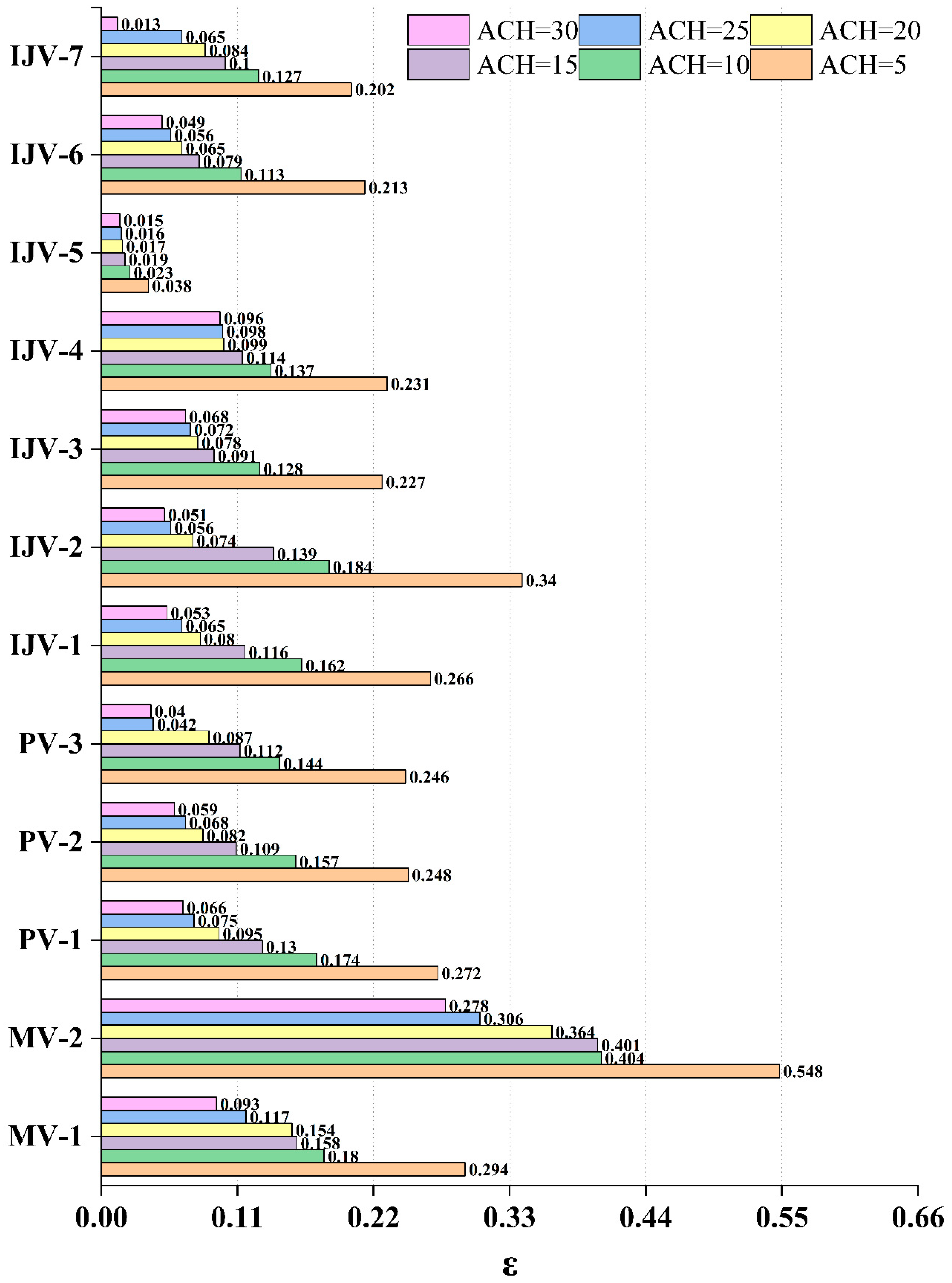
3.2. Performance of MV, PV, and IJV with Hydrogen Sulfide in the Occupied Zone

The normalized concentration of hydrogen sulfide is shown in Figure 7 (Z = 1.5 m). It can be seen from the figure that the normalized concentration of hydrogen sulfide gradually decreases with the increase in the ACH. Among the twelve schemes, the normalized concentration value of MV-2 is the highest; IJV-5 has the lowest normalized concentration value. When the ACH is 5, the hydrogen sulfide concentration cloud diagram of the Z = 1.5 m section is shown in Figure 8. The concentration in the toilet stall of MV-2 is high, and the concentration of hydrogen sulfide near the door hole and exhaust fan is low (Figure 8b); the gas velocity near the exhaust fan is large, the flow lines in the toilet stalls are sparse, and the hydrogen sulfide gas discharge effect is not good (Figure 4b). The normalized concentration value of IJV-5 is small, the concentration of hydrogen sulfide pollutants is low, and the concentration of pollutants in some areas of the toilet stalls is high (Figure 8l); the vent of this scheme is relatively close to the monitoring surface, and the monitoring surface is hydrogen sulfide. The gas concentration is relatively low.

When the ACH is 5, the normalized concentration values of IJV-2 are 0.34; the normalized concentration values of other schemes are less than 0.3. IJV-2 has exhaust air near the urinal, and hydrogen sulfide gas will diffuse from the stalls to the vicinity of the urinal (Figure 8g). The normalized concentration of MV-1 is 0.294. The concentration in the stalls is high because the baffle between the stalls hinders the flow of hydrogen sulfide gas, and the concentration of hydrogen sulfide gas in other positions is low (Figure 8a). The normalized concentration values of PV-1, PV-2, and PV-3 are 0.272, 0.248, and 0.246, respectively. When the toilet stall is exhausted (PV-3), a better ventilation effect can be obtained. The pollutant concentration in the toilet stalls of PV-1 and PV-2 is high, and the pollutant concentration in other areas is shallow (Figure 8c,d). PV-3 has a high pollutant concentration near the doorway (Figure 8e). The position of the air outlet of this scheme is relatively low, which is beneficial to the diffusion of hydrogen sulfide gas.

The normalized concentration value of IJV-1 is lower than IJV-2, which is 0.266. The two schemes use the same ventilation method near the toilet. The hydrogen sulfide gas is distributed in the toilet stalls (Figure 8f). The flow lines in the middle area of the toilet are relatively dense, with a high wind speed and low pollutant concentration (Figure 4f). The normalized concentration values of IJV-3, IJV-4, and IJV-5 are 0.227, 0.231, and 0.038, respectively. The height of the air outlet of the three schemes is different, and the pollutant concentration distribution law of the monitoring surface (Z = 1.5 m) is different (Figure 8h–j); the three solutions form a vortex in the toilet stalls, the airflow velocity is high, the streamline is dense, and the removal effect of hydrogen sulfide pollutant is good (Figure 4h–j). The normalized concentration value of IJV-6 is higher than that of IJV-7. The two schemes use the same ventilation method, but the position of the vent is different, and the pollutant concentration in the toilet stall near the vent is high (Figure 8k,l).

When ACH is 10, the normalized concentration values of MV-2 and IJV-5 are 0.404 and 0.023, respectively, and the normalized concentration values of the other schemes are less than 0.2. When ACH increases from 5 to 10, the normalized concentration drop in IJV-5 is less than 0.07, and the other plans’ normalized concentration value drop values are all greater than 0.07. The normalized concentration value of different plans is affected by the number of air changes. Increasing the number of air changes can be effective in removing hydrogen sulfide pollutants.

When the ACH is 15, the normalized concentration of MV-2 is the largest, and the hydrogen sulfide concentration in the toilet stall near the doorway is very high (Figure 9b). The ventilation in this area is not smooth, and the pollutant removal effect is not good. The normalized concentration values of IJV-3, IJV-5, and IJV-6 are 0.091, 0.019, and 0.079, respectively, and the normalized concentration values of other schemes are greater than 0.1. The area with high hydrogen sulfide concentration in other schemes is small, so the normalized concentration value is less than 0.2.

When the ACH increases from 10 to 15, the normalized concentration reduction values of different schemes are different; the maximum value is 0.048 (PV-2), and the minimum value is 0.003 (MV-2). When the ACH increases from 15 to 20, the maximum reduction in the normalized concentration of the twelve schemes is 0.065 (IJV-2), and the minimum is 0.002 (IJV-5). When the ACH increases from 20 to 25, the maximum reduction in the normalized concentration of the twelve schemes is 0.058 (MV-2), and the minimum value is 0.001 (IJV-4, IJV-5). When the ACH increases from 25 to 30, the maximum reduction in the normalized concentration the twelve schemes is 0.052 (IJV-7), and the minimum value is 0.001 (IJV-5). As the ACH increase, the reduction in the normalized concentration value becomes smaller.

The normalized concentration values of Z = 0.9 m and Z = 1.5 m cross-sections have similar changes. The normalized concentration value of MV-2 is the largest, and the normalized concentration value of IJV-5 is the smallest (under the same ACH) (Figure S7).

The normalized concentration values of different ventilation schemes are quite different (under the same number of air changes), increasing the number of air changes. The pollutant removal rate can be improved, but the indoor wind speed will increase accordingly, and the high indoor airspeed will affect the comfort of the toilet. MV is not as good as PV and IJV in reducing the normalized concentration value. Jet ventilation in the toilet stalls can effectively remove hydrogen sulfide gas and improve the IAQ in toilets.

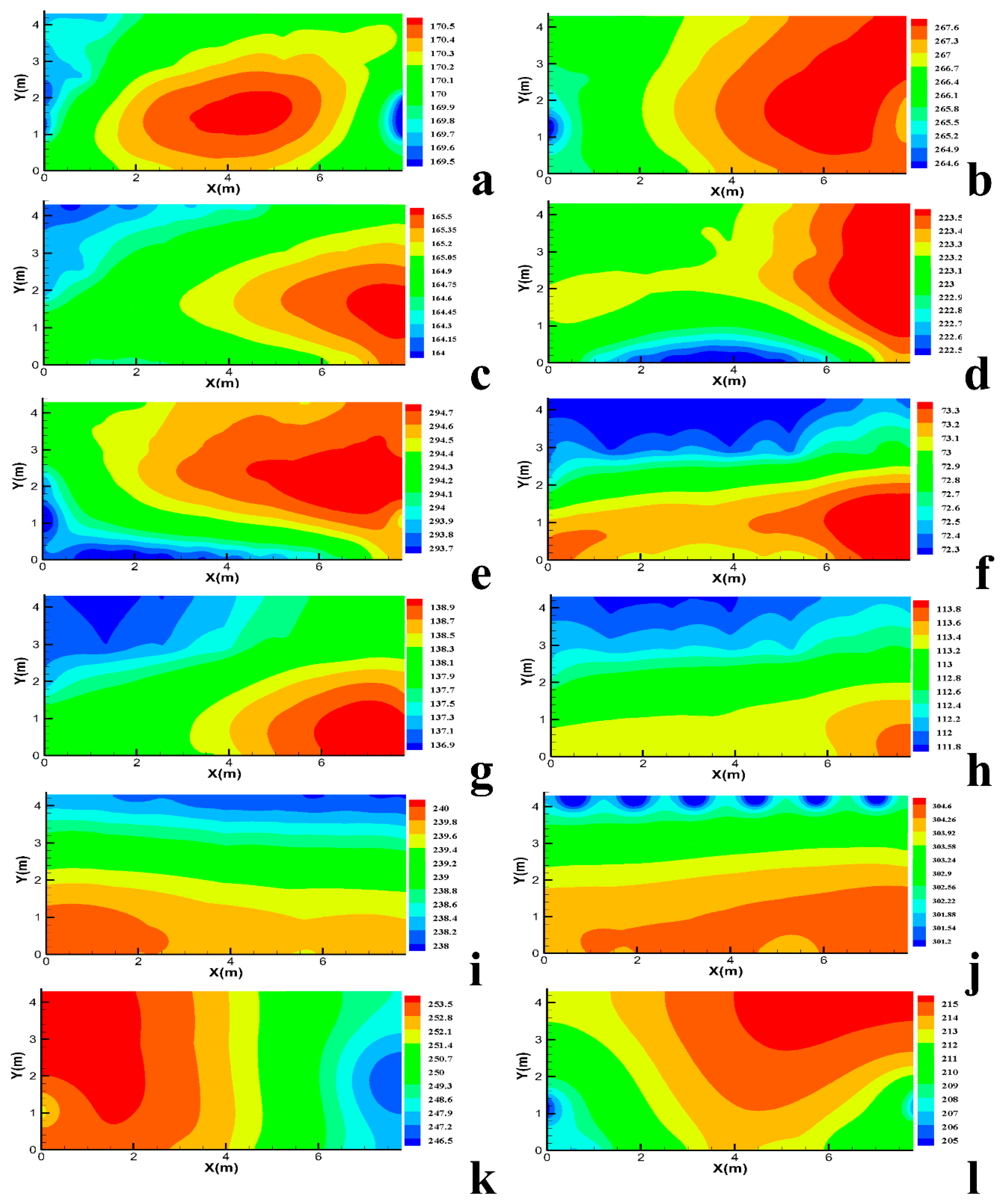
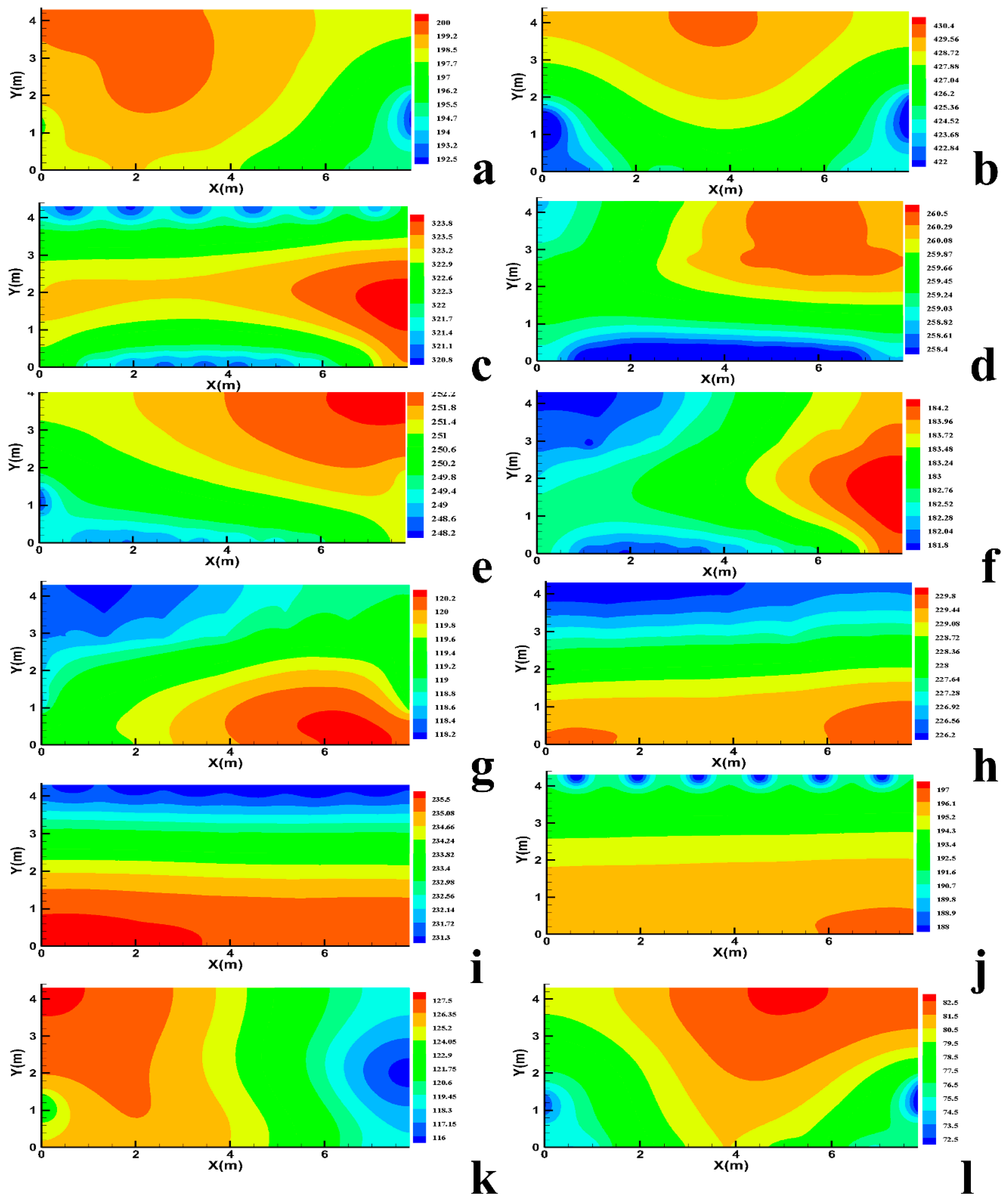
3.3. Air Age in the Occupied Zone under MV, PV, and IJV

The concept of MAA can be applied to pollutants or any tracer gas that simulates pollutants [64]. Assuming that pollutants are "born" when they enter the plenum, the local MAA at any point is the average time it takes for all pollutant particles to reach that point from the entrance area. This means that the "youngest" air is still at the air supply port, while the "oldest" air may be located in the stagnant zone or trapped in the air outlet [65]. If part of the air circulates in the stall for a long time, the local MAA value will increase significantly, so these values depend largely on the effectiveness of the ventilation system [66].

The error between CFD simulation results and experimental results is very small; the predicted value on the coarse grid is higher than the predicted value on the fine grid. The relative error of the average local average age in the coarse grid room is 4% [67].

The MAA of each program under different ventilation times is shown in Figure 10. When the ACH is the same, the MAA of different schemes is very different. When the ACH is 5, the maximum and minimum MAA are 304 (IJV-5) and 73 (IJV-1), respectively, which is a big difference. The MAAs of MV-1, PV-1, IJV-2, and IJV-3 are 170, 165, 138, and 113, respectively, and the MAAs of the other programs are greater than 200.

When the jet ventilation air supply outlet is higher than the monitoring surface (IJV-5), the MAA on the monitoring surface is long. The MAA in the area far away from the air supply is long (Figure 11j); when the air is supplied near the urinal (IJV-1), the air in the toilet stall is relatively fresh, and the MAA is short (Figure 11f); when the air is exhausted near the urinal (IJV-2), the air supply is reduced. The internal air circulation becomes slower, and the MAA becomes longer (Figure 11g). In the two schemes, the MAA at the corner of the wall becomes longer because these areas are prone to vortex flow, and the air circulation slows down. When the jet ventilation air outlet is low (IJV-3), the wind blows to the floor and then spreads upward. The MAA in the toilet stalls is very short, and the MAA in the area away from the toilet stalls becomes longer, but the average MAA is still very low (Figure 11h). The exhaust vents are evenly distributed on the top, and the middle area of the toilet is far away from the air intake and exhaust vents, so the MAA is longer (Figure 11a).

When air is supplied near the urinal, and near the toilet (PV-1), the MAA in the door area is long, and the other areas are short (Figure 11c); when the fan is on the sidewall (MV-2), the distance of the MAA is shorter in the area near the exhaust outlet, and the gas is more easily discharged (Figure 11b); when the air is supplied near the urinal and the air is exhausted near the toilet (PV-2, PV-3), the MAA in the area near the doorway is long and fresh air enters near the urinal. Hence, the MAA is short (Figure 11d,e). When the jet ventilation outlet is Z = 1.0 m (IJV-4), the MAA is long (Figure 11i). When using a jet air supply above the floor (IJV-6, IJV-7), the MAA near the air outlet is short, and the fresh air in the area far from the air outlet does not easily spread to this area, so the MAA is long (Figure 11k,l).

When the ACH is 10, the maximum and minimum MAAs are 474 (MV-2) and 94 (IJV-3), respectively. The MAAs of IJV-1, IJV-2, and IJV-7 are 143, 112, and 116, respectively. The MAAs of the other programs are all greater than 200 (Figure 10b). When the ACH increases from 5 to 10, the MAAs of IJV-2, IJV-3, IJV-5, IJV-6, and IJV-7 become smaller, while the MAAs of other programs become larger.

When the ACH is 15, the maximum and minimum MAAs are 307 (PV-1) and 83 (IJV-7), respectively. The MAAs of IJV-2 and IJV-6 are 120 and 123, respectively, with an age greater than 190. For PV-1 and IJV-1, the MAA at the doorway is long (Figure 12c,f), and for PV-2, PV-3, and IJV-7, the MAA above the toilet stall is long (Figure 12d,e,l). When ACH is 20, the maximum and minimum MAA are 289 (PV-3) and 60 (IJV-7), respectively. The MAA of IJV-1 is 93, and the MAA of the other programs is greater than 100. When ACH is 25, the maximum and minimum MAA are 211 (PV-2) and 45 (IJV-7). The MAA of IJV-6 is 86, and the other is not less than 100. When ACH is 30, the maximum and minimum MAA are 217 (IJV-4) and 37 (IJV-7), respectively. The MAA of IJV-6 is 69, and the other is greater than 100.

Increasing the number of air changes may lead to a longer MAA. Therefore, it is crucial to choose the right ACH for different schemes. In short, the IJV-7 program has the shortest MAA and the freshest air.

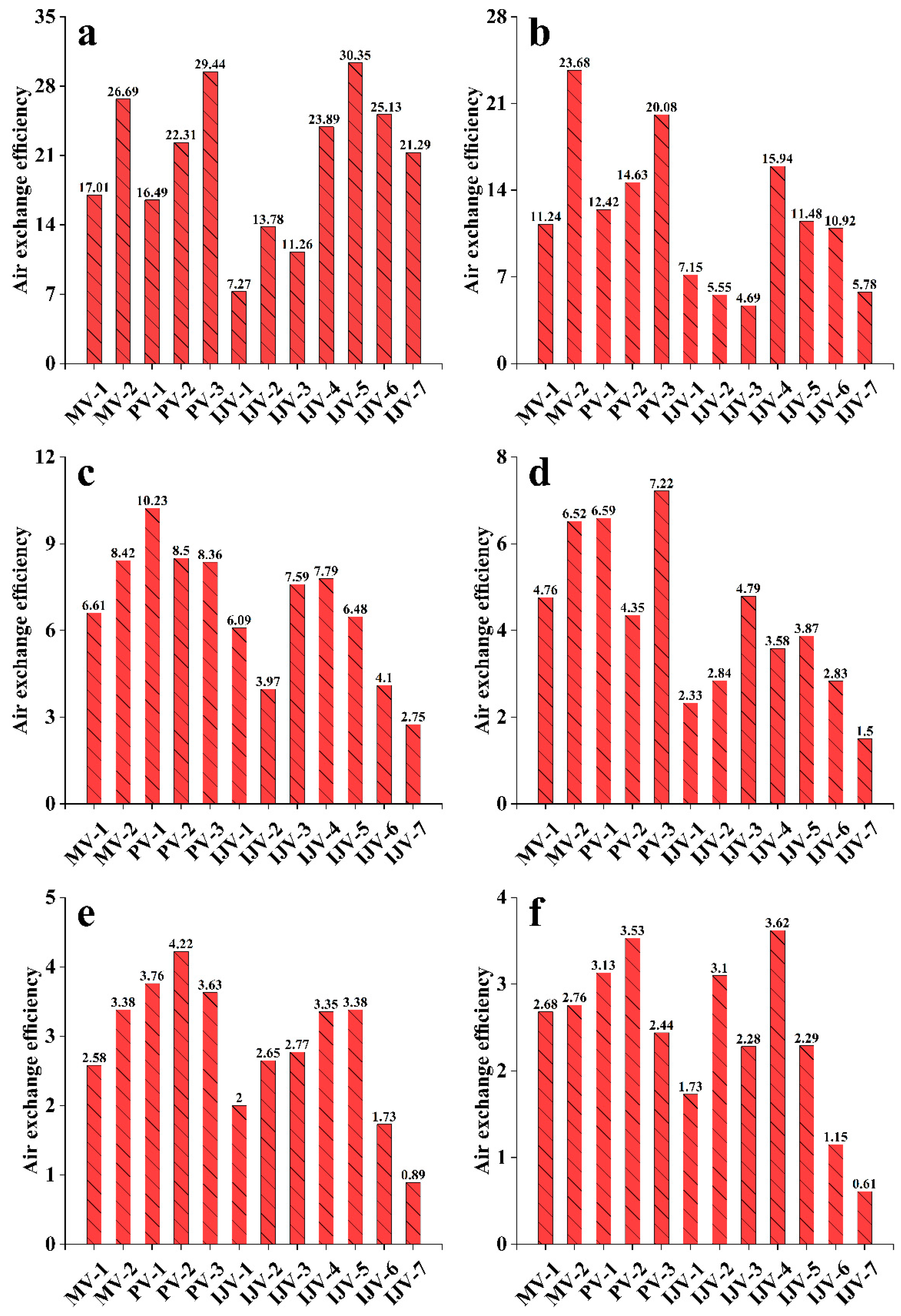
3.4. Air Exchange Efficiency in MV, PV, and IJV

The AEE of each scheme under different ventilation times is shown in Figure 9. When the ACH is 5, the maximum and minimum values of AEE are 30.35 (IJV-5) and 7.27 (IJV-1), respectively. The AEE values of MV-1, PV-1, IJV-2, and IJV-3 are 17.01, 16.49, 13.78, and 11.26, respectively, and the other schemes are greater than 20 (Figure 13a). The larger the AEE value, the higher the ventilation efficiency. The AEE value of IJV-5 is the largest because the location of the jet air outlet of this scheme is high, and the average MAA of the toilet is short; the airflow velocity at the corners is small, the MAA is longer, the average MAA of the toilet becomes longer, and the AEE value is minimal.

When the ACH is 10, the maximum and minimum values of the AEE are 23.675 (MV-2) and 4.685 (IJV-3), respectively. The AEEs of IJV-1, IJV-2, and IJV-7 are 7.145, 5.545, and 5.775, respectively. The AEEs of the other schemes are greater than 10 (Figure 13b). When the air outlet is located on the wall directly opposite the door hole (MV-2), the fresh air entering from the door hole is exhausted to the outside through the exhaust fan, and the gas flow path is short and inside the toilet stall. The average MAA is short, so the AEE value is large; when the jet vent position is low (IJV-3), the airflow velocity below the air outlet is large, the airflow velocity above the air outlet is small, and the MAA in the toilet is long, so the AEE value is small.

When the ACH is 15, the maximum and minimum values of the AEE are 10.23 (PV-1) and 2.75 (IJV-7), respectively, and the AEE of the other schemes is less than 9 (Figure 13c). When the whole air supply scheme is adopted (PV-1), the average MAA in the toilet is the shortest, and the AEE value is the largest. When air is supplied near the ground, the wind speed around the air outlet is high, and the flow velocity in the upper space of the toilet is small. Therefore, the average MAA in the toilet is the longest, and the AEE value is the smallest.

When the ACH is 20, the maximum and minimum values of AEE are 7.2165 (PV-3) and 1.4995 (IJV-7), respectively, and the AEE of the other schemes is less than 7 (Figure 13d). When the ACH is 25, the maximum and minimum values of AEE are 4.224 (PV-2) and 0.89 (IJV-7), respectively, and the AEE of the other schemes is less than 4 (Figure 13e). When the ACH is 30, the maximum and minimum values of the AEE are 3.62 (IJV-4) and 0.61 (IJV-7), respectively (Figure 13f).

As the number of ACH increases, the value of AEE gradually decreases, and the ventilation efficiency gradually decreases. When the ACH is 15, 20, 25, or 30, the AEE value of IJV-7 is the smallest. It is essential to choose a suitable ACH to improve the ventilation efficiency and reduce the concentration of pollutants.

4. Conclusions

CFD methods were used to investigate the normalized concentration in MV, PV, and IJV. The conclusions of this study are as follows:

• This study investigated the normalized concentrations of ammonia and hydrogen sulfide gas at the monitoring face under six ACHs (5h⁻¹, 10 h⁻¹, 15 h⁻¹, 20 h⁻¹, 25 h⁻¹, and 30 h⁻¹). The results show that the ventilation method, position of the air outlet and the supply air, and the ACH affect the concentration of pollutants. Increasing the ACH can reduce the normalized concentration of pollutants and improve the IAQ in public toilets.
• The mixed ventilation scheme is ineffective in removing pollutants, and IJV has advantages in reducing pollutants over PV and MV. IJV-7 performs best in reducing the normalized concentration of ammonia, and IJV-5 has an advantage in reducing the normalized concentration of hydrogen sulfide.
• Increasing the number of air changes may lead to a longer MAA. The IJV-7 program has the shortest MAA and the freshest air but the smallest AEE value. Therefore, it is vital to choose the correct number of air changes for different ventilation schemes.
• The research results of this paper supply a theoretical basis for improving ventilation efficiency. From the perspective of improving public health and the prevention of infectious diseases, this research is of great significance.

References

1. Zhu, S.; Zheng, X.; Stevanovic, S.; Wang, L.; Wang, H.; Gao, J.; Xiang, Z.; Ristovski, Z.; Liu, J.; Yu, M. Investigating particles, VOCs, ROS produced from mosquito-repellent incense emissions and implications in SOA formation and human health. Build. Environ. 2018, 143, 645–651. [Google Scholar] [CrossRef]
2. Lim, S.S.; Vos, T.; Flaxman, A.D.; Danaei, G.; Shibuya, K.; Adair-Rohani, H.; AlMazroa, M.A.; Amann, M.; Anderson, H.R.; Andrews, K.G.; et al. A comparative risk assessment of burden of disease and injury attributable to 67 risk factors and risk factor clusters in 21 regions, 1990–2010: A systematic analysis for the Global Burden of Disease Study 2010. Lancet 2012, 380, 2224–2260. [Google Scholar] [CrossRef] [Green Version]
3. He, X.; Zhou, G.; Ma, Y.; Li, L.; Luo, B. Winter vacation, indoor air pollution and respiratory health among rural college students: A case study in Gansu Province. China Build. Environ. 2020, 188, 107481. [Google Scholar] [CrossRef]
4. Murga, A.; Long, Z.; Yoo, S.J.; Sumiyoshi, E.; Ito, K. Decreasing inhaled contaminant dose of a factory worker through a hybrid Emergency Ventilation System: Performance evaluation in worst-case scenario. Energy Built Environ. 2020, 1, 319–326. [Google Scholar] [CrossRef]
5. Peng, B.Y.; Su, Y.; Chen, Z.; Chen, J.; Zhou, X.; Benbow, M.E.; Griddle, C.S.; Wu, W.M.; Zhang, Y. Biodegradation of Polystyrene by Dark (Tenebrio obscurus) and Yellow (Tenebrio molitor) Mealworms (Coleoptera: Tenebrionidae). Environ. Sci. Technol. 2019, 53, 5256–5265. [Google Scholar] [CrossRef]
6. Steinemann, A.; Wargocki, P.; Rismanchi, B. Ten questions concerning green buildings and indoor air quality. Build. Environ. 2016, 112, 351–358. [Google Scholar] [CrossRef] [Green Version]
7. Ben-David, T.; Rackes, A.; Lo, L.J.; Wen, J.; Waring, M.S. Optimizing ventilation: Theoretical study on increasing rates in offices to maximize occupant productivity with constrained additional energy use. Build. Environ. 2019, 166, 106314.1–106314.13. [Google Scholar] [CrossRef]
8. Boots, A.W.; Berkel, J.V.; Dallinga, J.W.; Smolinska, A.; Wouters, E.; Schooten, F.V. The versatile use of exhaled volatile organic compounds in human health and disease. J. Breath Res. 2012, 6, 027108. [Google Scholar] [CrossRef]
9. Sato, H.; Hirose, T.; Kimura, T.; Moriyama, Y.; Nakashima, Y. Analysis of malodorous volatile substances of human waste: Feces and urine. J. Health Sci. 2001, 47, 483–490. [Google Scholar] [CrossRef] [Green Version]
10. Ao, Y.; Wang, L.; Jia, X.; Gu, C. Numerical Simulation of Pollutant Diffusion Law in Bathroom and Optimization of the Locations and Ways of Exhaust Outlet and Makeup Air, Shenyang Jianzhu Daxue Xuebao (Ziran Kexue Ban). J. Shenyang Jianzhu Univ. 2011, 27, 720–724. [Google Scholar]
11. Sun, X.G. Hygienic Standards for Communal Toilet in City; Domestic-National Standards-State Administration for Market Regulation: Beijing, China, 1998.
12. Zhang, S.; Cheng, Y.; Oladokun, O.; Wu, Y.; Lin, Z. Improving Predicted Mean Vote with Inversely Determined Metabolic Rate. Sustain. Cities Soc. 2019, 53, 101870. [Google Scholar] [CrossRef]
13. Perez-Lombard, L.; Ortiz, J.; Maestre, I.R. The map of energy flow in HVAC systems. Appl. Energy 2011, 88, 5020–5031. [Google Scholar] [CrossRef]
14. Zhang, S.; Lin, Z.; Ai, Z.; Wang, F.; Cheng, Y.; Huang, C. Effects of operation parameters on performances of stratum ventilation for heating mode. Build. Environ. 2019, 148, 55–66. [Google Scholar]
15. Lin, Y.P. Natural Ventilation of Toilet Units in K–12 School Restrooms Using CFD. Energies 2021, 14, 4792. [Google Scholar] [CrossRef]
16. Tung, Y.C.; Hu, S.C.; Tsai, T.I.; Chang, I.L. An experimental study on ventilation efficiency of isolation room. Build. Environ. 2009, 44, 271–279. [Google Scholar] [CrossRef]
17. Tung, Y.C.; Hu, S.C.; Tsai, T.Y. Influence of bathroom ventilation rates and toilet location on odor removal. Build. Environ. 2009, 44, 1810–1817. [Google Scholar] [CrossRef]
18. Tung, Y.C.; Shih, Y.C.; Hu, S.C.; Chang, Y.L. Experimental performance investigation of ventilation schemes in a private bathroom. Build. Environ. 2010, 45, 243–251. [Google Scholar] [CrossRef]
19. Chung, S.C.; Lin, Y.P.; Yang, C.; Lai, C.M. Natural Ventilation Effectiveness of Awning Windows in Restrooms in K-12 Public Schools. Energies 2019, 12, 2414. [Google Scholar] [CrossRef] [Green Version]
20. Haghshenaskashani, S.; Sajadi, B. Evaluation of Thermal Comfort, IAQ and Energy Consumption in an Impinging Jet Ventilation (IJV) System with/without Ceiling Exhaust. J. Build. Eng. 2018, 18, 142–153. [Google Scholar] [CrossRef]
21. Lt, A.; Jg, A.; Zl, B.; Li, W.A.; Lz, A.; Gl, A.; Yw, A. A novel flow-guide device for uniform exhaust in a central air exhaust ventilation system. Build. Environ. 2019, 149, 134–145. [Google Scholar]
22. Zeng, L.; Liu, G.; Gao, J.; Du, B.; Wang, Y. A circulating ventilation system to concentrate pollutants and reduce exhaust volumes: Case studies with experiments and numerical simulation for the rubber refining process. J. Build. Eng. 2020, 35, 101984. [Google Scholar] [CrossRef]
23. Sui, X.; Tian, Z.; Liu, H.; Chen, H.; Wang, D. Field measurements on indoor air quality of a residential building in Xi’an under different ventilation modes in winter. J. Build. Eng. 2021, 42, 103040. [Google Scholar] [CrossRef]
24. Gautam, K.R.; Rong, L.; Iqbal, A.; Zhang, G. Full-scale CFD simulation of commercial pig building and comparison with porous media approximation of animal occupied zone. Comput. Electron. Agric. 2021, 186, 106206. [Google Scholar] [CrossRef]
25. Lv, L.; Zeng, L.; Wu, Y.; Gao, J.; Zhang, J. Effects of Human Walking on the Capture Efficiency of Range Hood in Residential Kitchen. Build. Environ. 2021, 196, 107821. [Google Scholar] [CrossRef]
26. Lv, L.; Gao, J.; Zeng, L.; Cao, C.; He, L. Performance assessment of air curtain range hood using contaminant removal efficiency: An experimental and numerical study. Build. Environ. 2020, 188, 107456. [Google Scholar] [CrossRef]
27. Sa, A.; Wc, A.; Ch, B.; Kg, C.; Ng, C. Influence of mixed and displacement air distribution systems’ design on concentrations of micro-particles emitted from floor or generated by breathing. J. Build. Eng. 2019, 26, 100855. [Google Scholar]
28. Cao, G.; Nilssen, A.M.; Cheng, Z.; Stenstad, L.I.; Radtke, A.; Skogås, J. Laminar airflow and mixing ventilation: Which is better for operating room airflow distribution near an orthopedic surgical patient? Am. J. Infect. Control 2019, 47, 737–743. [Google Scholar] [CrossRef] [PubMed]
29. Wang, L.; Dai, X.; Wei, J.; Ai, Z.; Fan, Y.; Tang, L.; Jin, T.; Ge, J. Numerical comparison of the efficiency of mixing ventilation and impinging jet ventilation for exhaled particle removal in a model intensive care unit. Build. Environ. 2021, 200, 107955. [Google Scholar] [CrossRef]
30. Xue, T.; Bla, B.; Ym, C.; Dong, L.C.; Yla, B.; Yong, C. Experimental study of local thermal comfort and ventilation performance for mixing, displacement and stratum ventilation in an office. Sustain. Cities Soc. 2019, 50, 101630. [Google Scholar]
31. Fange, P.O. Human requirements in future air-conditioned environments. In Advances in Building Technology; Elsevier: Amsterdam, The Netherlands, 2002; pp. 29–38. [Google Scholar]
32. Schiavon, S.; Melikov, A.K.; Sekhar, C. Energy analysis of the personalized ventilation system in hot and humid climates. Energy Build. 2010, 42, 699–707. [Google Scholar] [CrossRef]
33. Shen, C.; Gao, N.; Wang, T. CFD study on the transmission of indoor pollutants under personalized ventilation. Build. Environ. 2013, 63, 69–78. [Google Scholar] [CrossRef]
34. Cermak, R.; Melikov, A.K. Protection of occupants from exhaled infectious agents and floor material emissions in rooms with personalized and underfloor ventilation. Hvac&R Res. 2007, 13, 23–38. [Google Scholar]
35. Gao, N.; Zhang, H.; Niu, J. Investigating indoor air quality and thermal comfort using a numerical thermal manikin. Indoor Built Environ. 2007, 16, 7–17. [Google Scholar] [CrossRef]
36. He, Q.; Niu, J.; Gao, N.; Zhu, T.; Wu, J. CFD study of exhaled droplet transmission between occupants under different ventilation strategies in a typical office room. Build. Environ. 2011, 46, 397–408. [Google Scholar] [CrossRef]
37. Cermak, R.; Melikov, A.K.; Forejt, L.; Kovar, O. Performance of personalized ventilation in conjunction with mixing and displacement ventilation. Hvac&R Res. 2006, 12, 295–311. [Google Scholar]
38. Nielsen, P.V. Control of airborne infectious diseases in ventilated spaces. J. R. Soc. Interface 2009, 6, S747–S755. [Google Scholar] [CrossRef] [PubMed] [Green Version]
39. Ameen, A.; Cehlin, M.; Larsson, U.; Karimipanah, T. Experimental Investigation of the Ventilation Performance of Different Air Distribution Systems in an Office Environment—Heating Mode. Energies 2019, 12, 1835. [Google Scholar] [CrossRef] [Green Version]
40. Karimipanah, T.; Awbi, H.B. Theoretical and experimental investigation of impinging jet ventilation and comparison with wall displacement ventilation. Build. Environ. 2002, 37, 1329–1342. [Google Scholar] [CrossRef]
41. Qin, C.; Lu, W.Z. Effects of ceiling exhaust location on thermal comfort and age of air in room under impinging jet supply scheme. J. Build. Eng. 2021, 35, 101966. [Google Scholar] [CrossRef]
42. Ye, X.; Zhu, H.; Kang, Y.; Zhong, K. Heating energy consumption of impinging jet ventilation and mixing ventilation in large-height spaces: A comparison study. Energy Build. 2016, 130, 697–708. [Google Scholar] [CrossRef]
43. Ye, X.; Kang, Y.; Yang, F.; Zhong, K. Comparison study of contaminant distribution and indoor air quality in large-height spaces between impinging jet and mixing ventilation systems in heating mode. Build. Environ. 2019, 160, 106159. [Google Scholar] [CrossRef]
44. Chen, H.J.; Moshfegh, B.; Cehlin, M. Numerical investigation of the flow behavior of an isothermal impinging jet in a room. Build. Environ. 2012, 49, 154–166. [Google Scholar] [CrossRef]
45. Chen, H.; Moshfegh, B.; Cehlin, M. Computational investigation on the factors influencing thermal comfort for impinging jet ventilation. Build. Environ. 2013, 66, 29–41. [Google Scholar] [CrossRef]
46. Ameen, A.; Cehlin, M.; Larsson, U.; Karimipanah, T. Experimental Investigation of the Ventilation Performance of Different Air Distribution Systems in an Office Environment—Cooling Mode. Energies 2019, 12, 1354. [Google Scholar] [CrossRef] [Green Version]
47. Yao, S.; Yong, G.; Nan, J.; Liu, J. Experimental investigation of the flow behavior of an isothermal impinging jet in a closed cabin. Build. Environ. 2015, 84, 238–250. [Google Scholar] [CrossRef]
48. Cooper, D.; Jackson, C.D.; Launder, E.B.; Liao, X.G. Impinging jet studies for turbulence model assessment—I. Flow-field experiments. Int. J. Heat Mass Transf. 1993, 36, 2675–2684. [Google Scholar] [CrossRef]
49. Shi, Z.; Chen, Q. Experimental and computational investigation of wall-mounted displacement induction ventilation system. Energy Build. 2021, 241, 110937. [Google Scholar] [CrossRef]
50. Li, X.; Li, D.; Yang, X.; Yang, J. Total air age: An extension of the air age concept. Build. Environ. 2003, 38, 1263–1269. [Google Scholar] [CrossRef]
51. Aziz, M.A.; Gad, I.; Mohammed, E.; Mohammed, R.H. Experimental and numerical study of influence of air ceiling diffusers on room air flow characteristics. Energy Build. 2012, 55, 738–746. [Google Scholar] [CrossRef]
52. Jurelionis, A.; Gagytė, L.; Prasauskas, T.; Čiužas, D.; Krugly, E.; Šeduikytė, L.; Martuzevičius, D. The impact of the air distribution method in ventilated rooms on the aerosol particle dispersion and removal: The experimental approach. Energy Build. 2015, 86, 305–313. [Google Scholar] [CrossRef]
53. Buratti, C.; Palladino, D. Mean Age of Air in Natural Ventilated Buildings: Experimental Evaluation and CO2 Prediction by Artificial Neural Networks. Appl. Sci. 2020, 10, 1730. [Google Scholar] [CrossRef] [Green Version]
54. Ning, M.; Mengjie, S.; Mingyin, C.; Dongmei, P.; Shiming, D. Computational fluid dynamics (CFD) modelling of air flow field, mean age of air and CO2 distributions inside a bedroom with different heights of conditioned air supply outlet. Appl. Energy 2016, 164, 906–915. [Google Scholar] [CrossRef]
55. Chanteloup, V.; Mirade, P.-S. Computational fluid dynamics (CFD) modelling of local mean age of air distribution in forced-ventilation food plants. J. Food Eng. 2009, 90, 90–103. [Google Scholar] [CrossRef]
56. Ng, K.C.; Ng, E.Y.K.; Yusoff, M.Z.; Lim, T.K. Applications of high-resolution schemes based on normalized variable formulation for 3D indoor airflow simulations. Int. J. Numer. Methods Eng. 2010, 73, 948–981. [Google Scholar] [CrossRef]
57. Niachou, K.; Hassid, S.; Santamouris, M.; Livada, I. Experimental performance investigation of natural, mechanical and hybrid ventilation in urban environment. Build. Environ. 2008, 43, 1373–1382. [Google Scholar] [CrossRef]
58. Liu, M.; Chang, D.; Liu, J.; Ji, S.; Lin, C.H.; Wei, D.; Long, Z.; Zhang, T.; Shen, X.; Cao, Q.; et al. Experimental investigation of air distribution in an airliner cabin mockup with displacement ventilation. Build. Environ. 2021, 191, 107577. [Google Scholar] [CrossRef]
59. Gilani, S.; Montazeri, H.; Blocken, B. CFD simulation of stratified indoor environment in displacement ventilation: Validation and sensitivity analysis. Build. Environ. 2015, 95, 299–313. [Google Scholar] [CrossRef]
60. Shaojie, J.; Jinfeng, M. Pollutant Concentration Research of Toilet in Natural Ventilation Conditions. Contam. Control. Air Cond. Technol. 2012, 4, 22–24. [Google Scholar]
61. Yang, X.; Yang, H.; Ou, C.; Luo, Z.; Hang, J. Airborne transmission of pathogen-laden expiratory droplets in open outdoor space. Sci. Total Environ. 2021, 773, 145537. [Google Scholar] [CrossRef]
62. Etheridge, D.W.; Sandberg, M. Building Ventilation: Theory and Measurement; Wiley: Chichester, UK, 1996. [Google Scholar]
63. Lu, Y. HVAC HVAC Design Guidelines; China Construction Industry Press: Beijing, China, 1996. [Google Scholar]
64. Desta, T.Z.; Buggenhout, S.V.; Brecht, A.V.; Meyers, J.; Aerts, J.M.; Baelmans, M.; Berckmans, D. Modelling mass transfer phenomena and quantification of ventilation performance in a full scale installation. Build. Environ. 2005, 40, 1583–1590. [Google Scholar] [CrossRef]
65. Zhang, L.; Chow, T.T.; Fong, K.F.; Tsang, C.F.; Wang, Q. Comparison of performances of displacement and mixing ventilations. Part II: Indoor air quality. Int. J. Refrig. 2005, 28, 288–305. [Google Scholar]
66. Simons, M.W.; Waters, J.R. Ventilation effectiveness parameters resulting from mechanical ventilation with recirculation. Int. J. Ventil. 2002, 1, 119–126. [Google Scholar] [CrossRef]
67. Bartak, M.; Cermak, M.; Clarke, J.; Denev, J.; Drkal, F.; Lain, M.; Macdonald, I.; Majer, M.; Stankov, P. Experimental and numerical study of local mean age of air. In Proceedings of the 7th International Building Performance Simulation Association Conference, Rio de Janeiro, Brazil, 13–15 August 2001. [Google Scholar]
Figure 1. Geometry of the public toilet model: (a) vent positions in MV, PV, and IJV; (b) vent positions in IJV; (c) top view. 1—M1; 2—M2; 3—PV-U1; 4—PV-S1; 5—PV-S3; 6—J6, 7—J7; 8—J1; 9—Urinal; 10—Stall; 11—Window; 12—Window; 13—Door. M1, S2, S3, and M2 are outlet; J1, J2, J3, J6, J7, and S1 are inlet.
Energies 14 08379 g001
Figure 2. The normalized concentration of ammonia at Z = 1.5 m section.
Energies 14 08379 g002
Figure 3. Ammonia concentration cloud diagram in different cases (Z = 1.5 m, ACH = 5): (al) MV-1–IJV-7. (a): MV-1; (b): MV-2; (c): PV-1; (d): PV-2; (e): PV-3; (f): IJV-1; (g): IJV-2; (h): IJV-3; (i): IJV-4; (j): IJV-5; (k): IJV-6; (l): IJV-7.
Energies 14 08379 g003
Figure 4. Velocity vector contours in different cases (Z = 1.5 m, ACH = 5): (al) MV-1–IJV-7.
Energies 14 08379 g004
Figure 5. Ammonia concentration distribution for different cases (Z = 1.5 m, ACH = 15): (al) MV-1–IJV-7.
Energies 14 08379 g005
Figure 6. Velocity vector contours in different cases (Z = 1.5 m, ACH = 15): (al) MV-1–IJV-7.
Energies 14 08379 g006
Figure 7. The normalized concentration of hydrogen sulfide at Z = 1.5 m section.
Energies 14 08379 g007
Figure 8. Hydrogen sulfide concentration distribution for different cases (Z = 1.5 m, ACH = 5): (al) MV-1– IJV-7.
Energies 14 08379 g008
Figure 9. Hydrogen sulfide concentration distribution for different cases (Z = 1.5 m, ACH = 15): (al) MV-1–IJV-7.
Energies 14 08379 g009
Figure 10. Air age in different scenarios (af): ACH = 5–30.
Energies 14 08379 g010
Figure 11. Air age cloud diagrams of different scenarios (ACH = 5), (al) MV-1 – IJV-7.
Energies 14 08379 g011
Figure 12. Air age cloud diagrams of different scenarios (ACH = 15), (al) MV-1 – IJV-7.
Energies 14 08379 g012
Figure 13. Air exchange efficiency in different scenarios, (af): ACH = 5–30.
Energies 14 08379 g013