Assessment of Machine-Learned Turbulence Models Trained for Improved Wake-Mixing in Low-Pressure Turbine Flows

Abstract

This paper presents an assessment of machine-learned turbulence closures, trained for improving wake-mixing prediction, in the context of LPT flows. To this end, a three-dimensional cascade of industrial relevance, representative of modern LPT bladings, was analyzed, using a state-of-the-art RANS approach, over a wide range of Reynolds numbers. To ensure that the wake originates from correctly reproduced blade boundary-layers, preliminary analyses were carried out to check for the impact of transition closures, and the best-performing numerical setup was identified. Two different machine-learned closures were considered. They were applied in a prescribed region downstream of the blade trailing edge, excluding the endwall boundary layers. A sensitivity analysis to the distance from the trailing edge at which they are activated is presented in order to assess their applicability to the whole wake affected portion of the computational domain and outside the training region. It is shown how the best-performing closure can provide results in very good agreement with the experimental data in terms of wake loss profiles, with substantial improvements relative to traditional turbulence models. The discussed analysis also provides guidelines for defining an automated zonal application of turbulence closures trained for wake-mixing predictions.

1. Introduction

In order to face the global challenge of containing climate change effects, the International Civil Aviation Organization (ICAO) set out climate protection targets for global air transport. Starting from 2020, air traffic shall only be expanded pursuing a carbon-neutral growth. The ultimate goal is to cut CO₂ emissions from air transport in half by 2050, compared to the base year of 2005, in order to keep global warming below 1.5 ${}^{°}$C as recommended by the Intergovernmental Panel on Climate Change (IPCC) [1]. In 2018, commercial airliners consumed approximately 360 billion liters of aviation fuel globally (source: www.statista.com (accessed on July 2019)). The reduction of specific fuel consumption directly impacts the carbon footprint of aeroengines and thus remains one of the primary objectives for the aviation industry. In addition to that, aircraft noise is the most significant cause of adverse community reaction related to the operation and expansion of airports. Noise reduction at the source has proven to be effective, and it remains a priority for aircraft engine manufacturers.

One of the most important components of a turbofan engine is the low-pressure turbine (LPT). Improving the design of LPTs is of direct relevance to the aviation industry; primarily for the fact that if the efficiency of an LPT increases by 1%, the specific fuel consumption decreases by a fraction of about 0.6–0.8% (Michelassi et al., [2]). LPTs are characterized by Reynolds numbers that can vary from some hundred thousands at take-off to less than ${10}^5$ at cruise conditions. A large portion of the blade boundary-layer remains laminar, and transition may occur due to separated flow on the suction side of highly loaded bladerows. Any enhancement of physics-based, predictive modeling of transition, turbulence, and separation, allowing optimization of the flow details, can translate to huge savings in fuel consumption.

Reynolds-averaged Navier–Stokes (RANS) approaches remain the primary tools in turbomachinery design as they are highly cost effective, thus enabling designers to run several parametric studies and optimizations at acceptable computational costs. The major drawback of the RANS framework regards its inaccuracy as compared to high-fidelity simulations such as direct numerical simulation (DNS) or large eddy simulation (LES), so that it appears sometimes inadequate to predict the flow details. High-fidelity simulations are able to provide remarkably new insights into the flow physics. This however happens typically at the base research level and on the single blade row or stage, but the penetration in design practices is still very limited, since such approaches are several orders of magnitude more expensive than traditional ones. For multidisciplinary optimization of entire turbine or compressor modules for the next generation of gas turbine engines, designers are oriented to URANS simulations for rotor–stator interaction analyses in multistage environments. There is a strong industrial interest in the improvement of the prediction capabilities of such methodologies.

One of the flow features that clearly shows poor reproduction by RANS/URANS methods, and that is receiving considerable attention nowadays, is the wake-mixing phenomenon [3,4]. Wake/boundary-layer interactions are the main drivers for unsteady transition in LPTs [5,6], which is a crucial flow feature, especially for high-lift airfoils often sought after by designers in order to reduce weight and cost. They are also a major driver for tone noise generation by the LPT [7,8,9]. The numerical results reported in [10] represent just one example of not completely satisfactory reproduction of wake loss profiles in LPT flows. A proper representation of the wake evolution is expected to contribute remarkably to the accuracy of traditional CFD approaches in this context.

Recently, major attention has been devoted to the possibility offered by the exploitation of high-fidelity analyses to improve the accuracy of existing RANS/URANS methods. To this end, machine-learning techniques driven by LES, DNS results, appears a very attractive mean to improve turbulence and transition closures [11]. Weatheritt and Sandberg [12] developed gene expression programming (GEP) [13] for turbulence modeling, which creates new explicit algebraic Reynolds stress models (EARSM) that inherently satisfy Galilean invariance based on high-fidelity databases. Akolekar et al. [14,15] used such a machine learning framework to develop EARSMs for enhanced wake-mixing predictions in LPTs, with steady and unsteady inlet flow conditions. Zhao et al. [16] introduced the concept of the ’CFD-driven’ approach to GEP-based turbulence model development. ’CFD-driven’ training enables the definition of the cost function that can be tailored to capture any important flow feature of interest, instead of being restricted to quantities that are strictly part of the closure terms (e.g., the anisotropy tensor). Such a strategy has proven to be encouraging to generate EARSM closures for improved wake-mixing predictions in LPTs [17]. Finally, Lav et al. [18] developed a framework using GEP to produce data-driven turbulence models for flows with organized (deterministic or periodic) unsteadiness, thus paving the way for the application of data-driven turbulence modeling to URANS approaches for rotor–stator interaction studies.

In the present work, the performance of machine-learned EARSMs trained for improved wake-mixing predictions by RANS simulations are scrutinized against experimental data taken on a three dimensional cascade, designed by Avio Aero to be representative of a modern LPT vane for aeroengine applications. The assessment is carried out over a Reynolds number range that is typical of aeronautical LPTs operation, from take-off to cruise conditions. In such a range, the boundary layer developing on the investigated cascade undergoes a separated flow transition, and in order to ensure that the wake is fed by realistically reproduced blade boundary-layers, different transition models were considered and assessed against measured blade loading distributions. This allows checking for the correct prediction of separation, transition, and reattachment locations. To this end, two state-of-the-art transition modeling frameworks were considered: the $\gamma -R{e}_{\theta t}$ by Langtry and Menter [19] and the Laminar kinetic energy (LKE) transport approach proposed by Pacciani et al. [20], which have both been coupled with the Wilcox $k-\omega$ model [21]. The results show how the LKE model, which was explicitly devised for separated flow transition, yields superior accuracy in both the cases of mildly or strongly separated flow.

The GEP-based EARSMs were trained in the far wake region and are not suitable for wall bounded flows, so that their application requires a zonal strategy. A suitable “sensing function” would then be desirable to identify the flowfield regions where the machine-learned closures should be active. However, the present work is focused on assessing the performance of the models on a test case of industrial footprint based on a single-blade cascade, and the effort to define an automated zonal approach for the activation of the EARSMs was considered untimely. Rather, one of the goals of the paper is to address the definition of such a function by identifying some guidelines to avoid the application of the models in regions where they would lead to nonphysical behavior of the simulations (e.g., boundary-layers) or could impair the prediction of specifical flow features (e.g., secondary flows). In the present work, GEP-based EARSMs were applied only in the portion of the computational domain that extends between the blade trailing edge and the outlet boundary in the axial direction (to mask the blade boundary-layer), and between the $5\%$ and $95\%$ of the blade height in the spanwise direction (to mask the endwall boundary-layers). It must be pointed out that in some cases [17] the training region of the models starts in the far-wake and so their application in the near wake could appear questionable. However, the task of defining a sensing function that distinguishes between the near and the far wake has a little probability of success. In order to check for the response of the models to the axial position where their activation starts, a sensitivity analysis to this parameter is presented and discussed in terms of comparisons between predicted and measured wake loss profiles. Finally, the impact of the machine-learned closure on the cascade secondary flow reproduction is presented and discussed in comparison with experimental data. It is shown how the use of a carefully selected GEP-based EARSM can substantially improve wake-mixing and integrated loss prediction over the whole analyzed Reynolds number range. This is expected to be a significant contribution for more realistic unsteady wake-induced transition simulations in rotor–stator interaction analyses, with potential impact on aerodynamic performance, efficiency, and noise emissions of the next generation of LPTs.

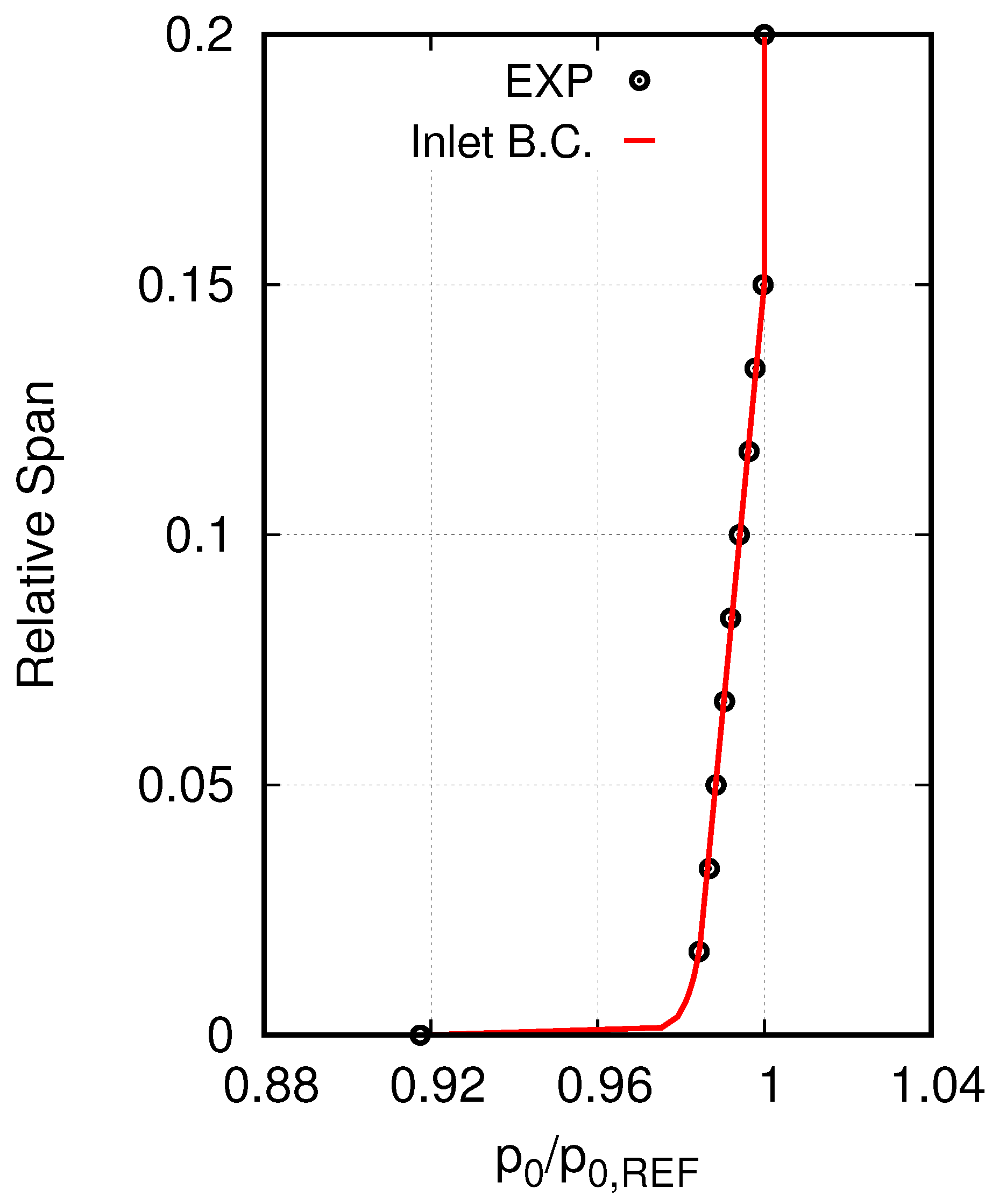
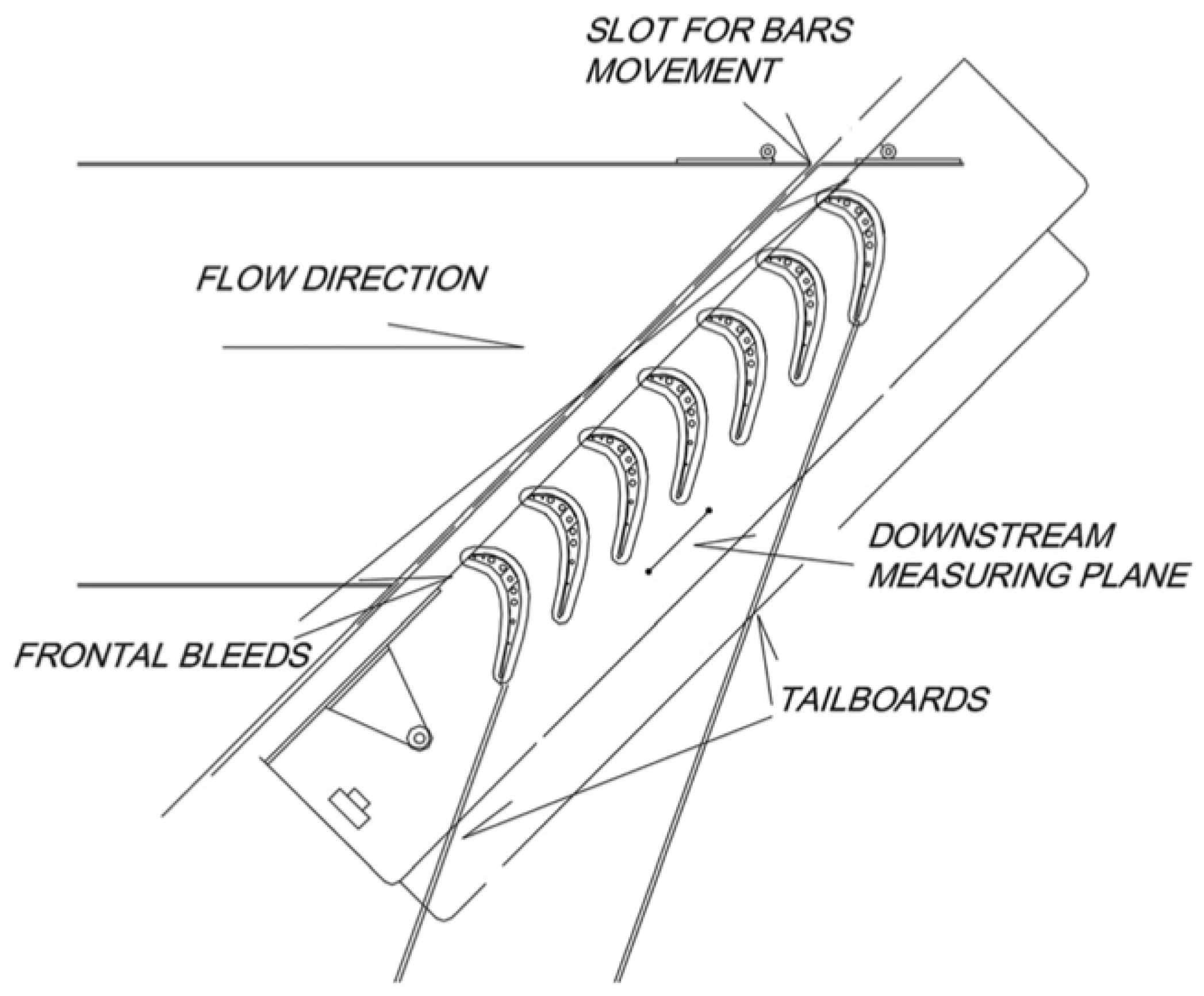
2. Test Case and Boundary Conditions

The cascade analyzed in the present work is representative of a modern LPT vane for aeroengine applications, in terms of blade loading distribution, pitch/chord ratio, Zweifel coefficient, suction side diffusion rate, and aspect ratio (see

Table 1. Cascade Parameters.

Zw	DR	AR
1.1	0.5	3.0

).

It features a three-dimensional design with increased chord near the endwalls in order to achieve higher solidity and reduced blade loading in these regions, thus offering potential for the reduction of secondary losses.

The cascade was experimentally investigated in the blow-down wind tunnel installed at the Aerodynamics and Turbomachinery Laboratory of the University of Genova under a variety of Reynolds number values and inlet conditions in terms of FSTI and endwall boundary-layer velocity profile. It consists of seven large-scale blades with an axial chord length of 100 mm as shown in Figure 1 that reports a sketch of the test rig. Further details on the experimental set-up can be found in Simoni et al. [22] and Marconcini et al. [23]. The measurement campaign considered for the present study comprises 4 exit isentropic Reynolds number values: $0.7\times {10}^5$, $1.0\times {10}^5$, $1.5\times {10}^5$, and $3.0\times {10}^5$. The exit isentropic Mach number was about $0.1$; therefore, the flow through the cascade was essentially incompressible. Inlet freestream turbulence was generated by a grid placed upstream the cascade, and the FSTI considered for the present analysis has a value of $4.2\%$ at the cascade leading edge. For the turbulent length scale, a nondimensional value of ${\ell }_T/L_{ref}=1.6\times {10}^{-3}$, where the axial chord at hub is assumed as the reference length, was adopted on the basis of previous experiences on the same test rig and experimental set-up (Giovannini et al. [24]).

The inlet endwall boundary layer was characterized by measuring the velocity profile upstream of the blade leading edge. Static pressure measurements in the same location allowed to translate the velocity profile into a spanwise total pressure distribution to be prescribed as a boundary condition for 3D RANS calculations. Giovannini et al. [24] has demonstrated how a lack of near wall resolution in the inlet boundary layer total pressure profile can lead to a relevant misrepresentation of the secondary flow in the cascade. A poor representation of near-wall features is quite typical in the experimental characterization of endwall boundary layers in wind tunnels, as velocity measurements can seldom be carried out below some percent of the blade span from the endwall. In the experimental campaign considered in the present work, the wall distance of the first point in the measured velocity profile is about the $2\%$ of the normalized blade span. Although the present work was not explicitly targeted at secondary flow analysis, there was a strong interest in determining whether and how the machine-learned EARSMs impact the predicted secondary vortices structure. To allow the realistic representation of secondary flow features needed for such a purpose, the procedure suggested in [24] was adopted in order to create a suitable inlet total pressure profile from the available experimental data. A power law is used to fit the measured velocity profile in such a way that the first point near to the wall lies below $z^{+}=100$. The resulting inlet total pressure profile is compared to the experimental one in Figure 2.

3. Domain Discretization

The cascade flow domain was discretized using an O-H grid with 621 mesh points on the blade surface, 101 in the pitchwise direction and 80 along half the blade span (the blade is symmetric in the spanwise direction) for a total of about 11M cells. The H block, stitched to the outlet boundary of the O mesh, is characterized by uniform mesh spacing in the axial and tangential directions in order to allow optimal resolution in the wake region and a realistic prediction of the mixing phenomenon. The grid structure and density were selected on the basis of previous experience and validation for cascade flows in incompressible and subsonic conditions and low or moderate Reynolds number [4,17,25,26]. For the Reynolds numbers considered in the present work, the $y^{+}$ value of the grid nodes closest to the blade surface is between 1 and 2. The value of $z^{+}$ along the endwalls is around 10.

4. Computational Framework

The TRAF code (Arnone [27]) was used for all the calculations presented in the paper. It is an in-house developed, density-based, RANS/URANS solver. Incompressible flows are handled via the artificial compressibility method proposed by Chorin [28]. In terms of numerical fluxes, a formally third-order TVD framework, based on the generalized min-mod limiter [29], built on top of the Roe upwind scheme, was employed.

Two different turbulence/transition frameworks, both based on the Wilcox $k-\omega$ model [21], are considered in the present work. In the first one, the turbulence model is coupled with the Langtry and Menter $\gamma -{\widetilde{Re}}_{\theta ,t}$ [19] model for transition prediction. In the second one, transition is treated via the laminar-kinetic-energy transport framework proposed by Pacciani et al. [20,30,31].

Such transition/turbulence modeling strategies have been coupled with machine-learned EARSMs for improved wake-mixing predictions. Following Weatheritt and Sandberg [12], the approach proposed by Pope [32] is used to decompose the Reynolds stress tensor into isotropic and anisotropic contributions:

$${\tau }_{ij}=\underset{isotropic}{\underbrace{\frac{2}{3}\rho k{\delta }_{ij}}}-\underset{anisotropic}{\underbrace{2{\mu }_T{S}_{ij}+2\rho k{a}_{ij}}}$$

(1)

where the anisotropy tensor $a_{ij}$ can be conveniently expressed in terms of a tensor basis $V_{ij}^{\left(n\right)}$ and scalar invariants $I_k$ that are functions of the nondimensional strain and rotation rate tensors $\tau S_{ij}$ and $\tau {\mathrm{\Omega }}_{ij}$, with $\tau =1/\omega$ being the turbulent time scale. A cubic closure, which is obtained by limiting the considered tensor basis elements to three, has proven to be an effective compromise between computational requirements and accuracy for wake evolution predictions in turbomachinery flows [16,17]. With such assumptions, the anisotropy tensor is formulated as:

$$a_{ij}=\sum _{n=1}^3{b}_n(I_1,I_2,I_3,...)V_{ij}^{\left(n\right)}$$

(2)

the selected tensor basis elements and invariants are expressed as:

$$V_{ij}^{\left(1\right)}=\tau S_{ij},V_{ij}^{\left(2\right)}={\tau }^2(S_{ik}{\mathrm{\Omega }}_{kj}-{\mathrm{\Omega }}_{ik}{S}_{kj}),V_{ij}^{\left(3\right)}={\tau }^2(S_{ik}{S}_{kj}-\frac{1}{3}{\delta }_{ij}{S}_{lm}{S}_{ml})$$

(3)

$$I_1={\tau }^2{S}_{lm}{S}_{ml},I_2={\tau }^2{\mathrm{\Omega }}_{lm}{\mathrm{\Omega }}_{ml}$$

(4)

Two closure relations were compared in the present work. The first one, which is referred to as GEP Y, is formulated as:

$$a_{ij}=(-2.57+I_1)V_{ij}^{\left(1\right)}+(-4)V_{ij}^{\left(2\right)}+(-0.11+0.09I_1{I}_2+I_1{I}_2)V_{ij}^{\left(3\right)}$$

(5)

and was proposed by Zhao et al. [16]. The training environment for this model comprised several turbine cascades at different Reynolds numbers; therefore, it was considered as a good candidate to be tested for improved wake mixing. The second closure, which is referred to as GEP H, was proposed by Akolekar et al. [17] and explicitly developed for LPT flows. It is expressed as:

$$a_{ij}=(-2)V_{ij}^{\left(1\right)}+(-2+I_2)V_{ij}^{\left(2\right)}+(-I_2)V_{ij}^{\left(3\right)}$$

(6)

Both the models showed extremely good agreement with LES and DNS results in their training environments in terms of wake loss profiles for several axial locations downstream of the cascades trailing edge.

Inlet boundary conditions were imposed in terms of span-wise distribution of flow angles, total pressure, turbulence intensity and length scale. The prescribed total pressure profile corresponds to that in Figure 2. A uniform distribution was prescribed for the flow angles and turbulence quantities. A constant static pressure was imposed on the domain outlet boundary. The cascade is symmetrical in the spanwise direction so the computational domain extends to one half of the blade height and symmetry conditions are imposed at midspan.

5. Discussion of Results

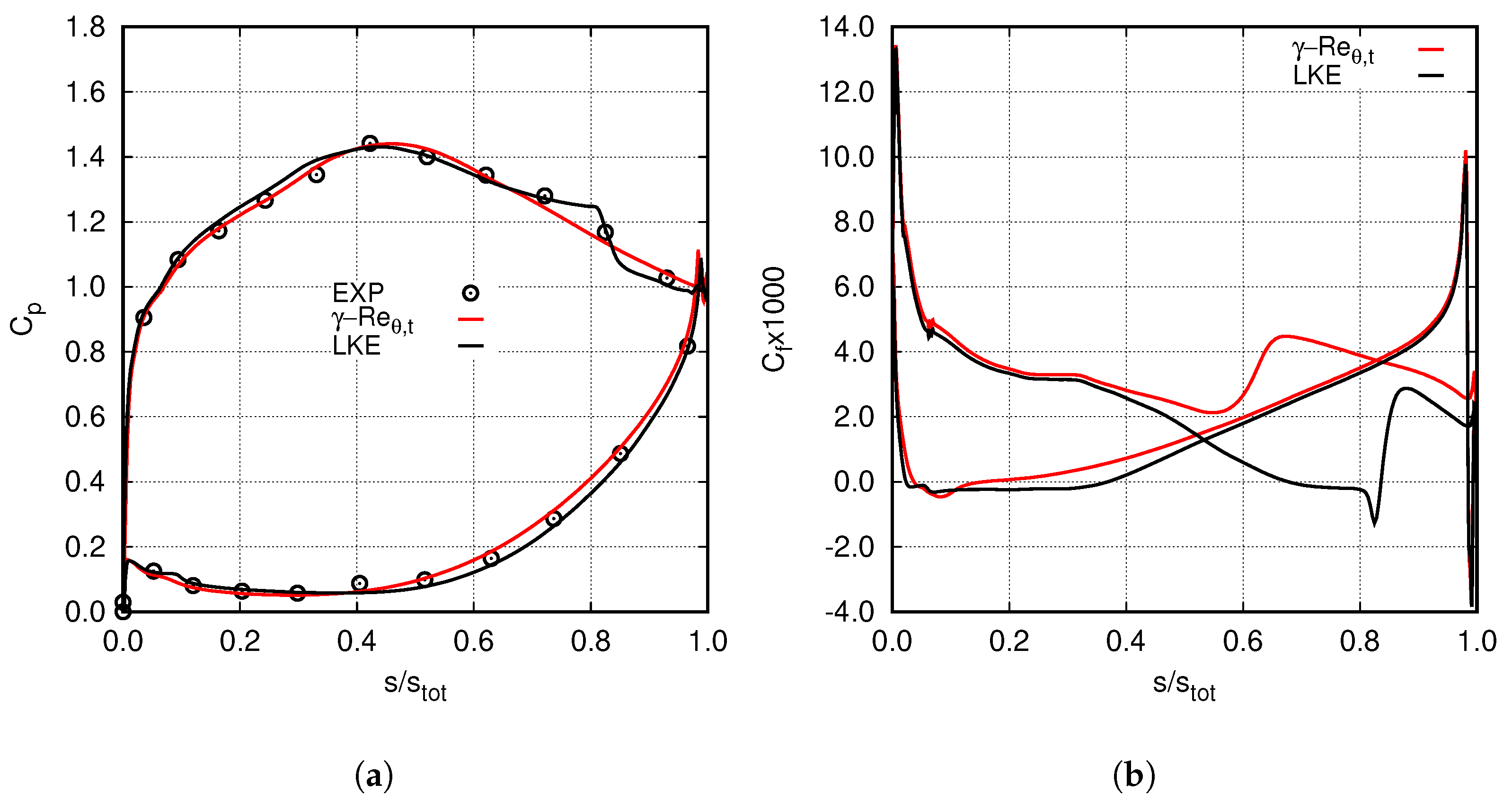
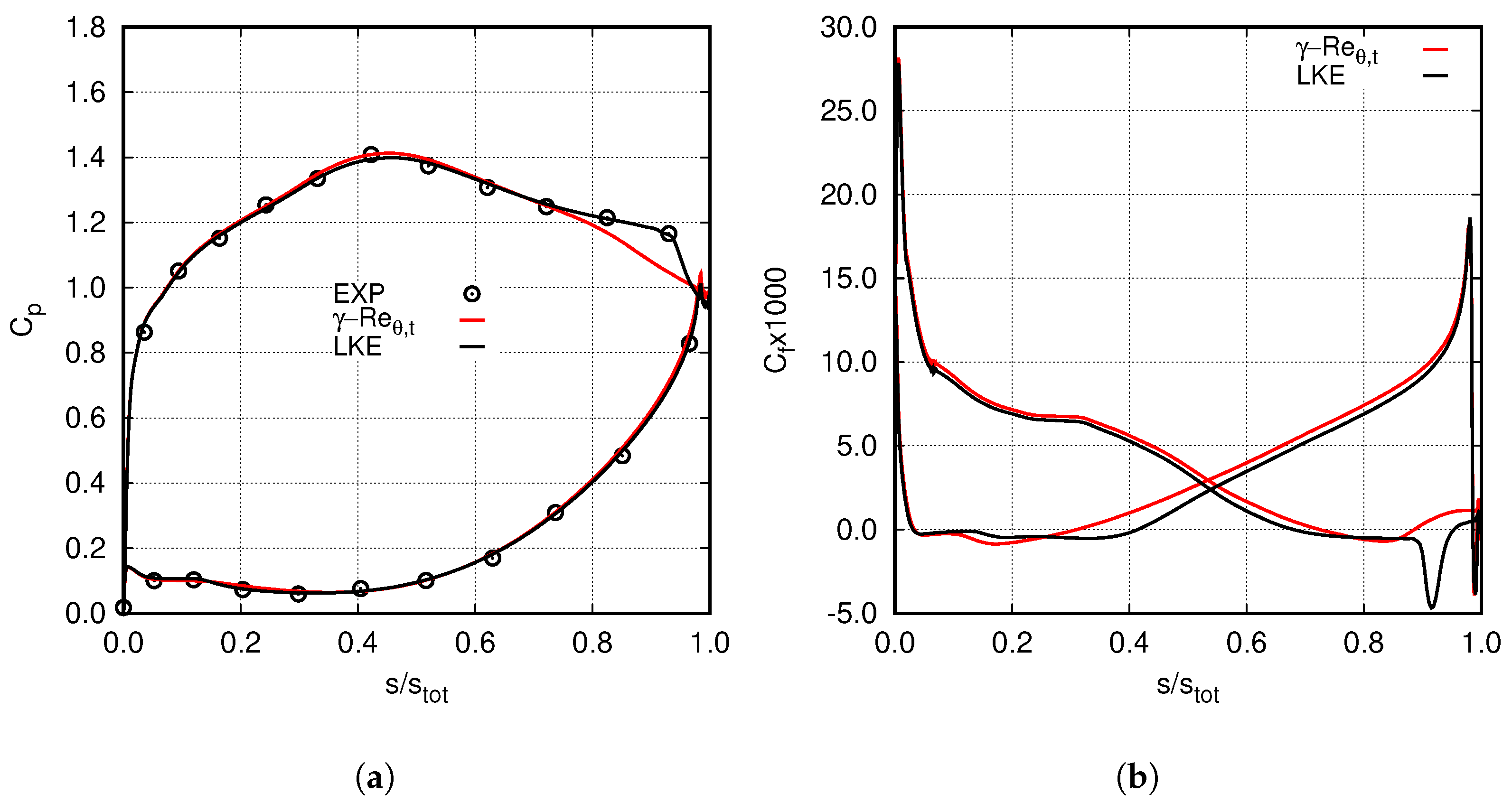
5.1. Blade Boundary-Layers and Effect of Transition Modelling

As mentioned previously, the paper focuses on the study of wake mixing and the related loss. For the assessment of the performance of the nonlinear EARSMs, it is important that the prediction of the wake structure by the RANS calculations is as realistic as possible. The fact that the wake originates from reasonably well reproduced blade surface boundary layers is a basic requirement. In the analyzed Reynolds number range, transition is expected to play a crucial role in determining the boundary layer details at the trailing edge. For such a reason, precursor calculations were carried out for the purpose of assessing the capabilities of the baseline modeling frameworks (without the machine-learned EARSMs) to correctly predict the transition mode and location. For the highest Reynolds number value in the investigated range ($R{e}_{2,is}=3.0\times {10}^5$), the computed blade loading distributions are compared with measurements in Figure 3a. They are reported in terms of pressure coefficient:

$$C_p=\frac{p_{01}-p\left(s\right)}{p_{01}-p_2}$$

(7)

as a function of the normalized surface length.

The two predictions are in substantial agreement and compare well with experimental data except in the last $30\%$ of the blade suction side length where discrepancies appear. The calculations carried out with the $\gamma -R{e}_{\theta ,t}$ model seem to underestimate the experimental $C_p$ in the uncovered part of the blade suction side, downstream of the throat up to the trailing edge. The reason for this can be made clear on the base of Figure 3b, which reports the calculated blade surface skin friction distributions. The skin-friction coefficient is here defined as:

$$C_f=\frac{2{\tau }_w}{\rho v_{REF}^2}$$

(8)

On the blade suction side, the $\gamma -R{e}_{\theta ,t}$ model predicts by-pass transition at about $60\%$ of the suction surface length, just after the suction velocity peak, thus keeping the wall shear stress high in almost the whole portion of the boundary layer subjected to adverse pressure gradient. This prevents a relevant blockage to develop downstream of the blade throat and promotes the smooth pressure recovery visible in the $\gamma -R{e}_{\theta ,t}$ solution. It is believed that the $\gamma -R{e}_{\theta ,t}$ model, for the quite high turbulence intensity characterizing the test case, tends to anticipate the transition onset. In the LKE solution, a separation bubble forms between the $65\%$ and the $85\%$ of the blade suction side length (Figure 3b). Separated flow transition occurs at about $s/S_{tot,ms}=0.82$, resulting in quite a sharp reattachment. The LKE results agree fairly well with the measured $C_p$ distribution. Although not reported in this paper, previous unpublished LES studies resolved a separation bubble of extension and topology similar to the one captured by the LKE model, and they were also in excellent agreement with the experimental data. On the blade pressure side, both the transition models predict separated flow transition due to the “cove” separation detectable in Figure 3b. The different sizes of the separated flow region, which can be appreciated in Figure 3b, result in different $C_p$ distributions that do not depict a clear winner between the two transition models in terms of agreement with experimental data.

It must be pointed out that the experimental resolution is not high enough to allow a definitive scrutiny of the investigated transition models in terms of calculated pressure coefficient distribution, at least at this Reynolds number. In order to shed more light on the relative merits of the two frameworks, the comparison was repeated for the lowest Reynolds number in the investigated range ($R{e}_{2,is}=0.7\times {10}^5$). The results of such an analysis are summarized in Figure 4a,b in terms of $C_p$ and $C_f$ blade surface distributions. At this Reynolds number, the presence of a separation bubble located on the blade suction side is evident in the measurements between $s/s_{tot,ms}=0.65$ and $s/s_{tot,ms}=0.9$ (Figure 4a).

The experimental pressure coefficient distribution is satisfactorily matched by the LKE calculation. The $\gamma -R{e}_{\theta ,t}$ model also predicts separated flow transition at such a Reynolds number, but, as it can be appreciated in Figure 4b, the size of the reproduced separation bubble is very small and does not introduce enough blockage for the pressure distribution to be sensibly influenced like it happens in the experiments.

On the basis of these results, the LKE model was deemed to predict a more realistic boundary layer behavior relative to the $\gamma -R{e}_{\theta ,t}$ framework, and it was adopted for the analyses that are discussed in the following.

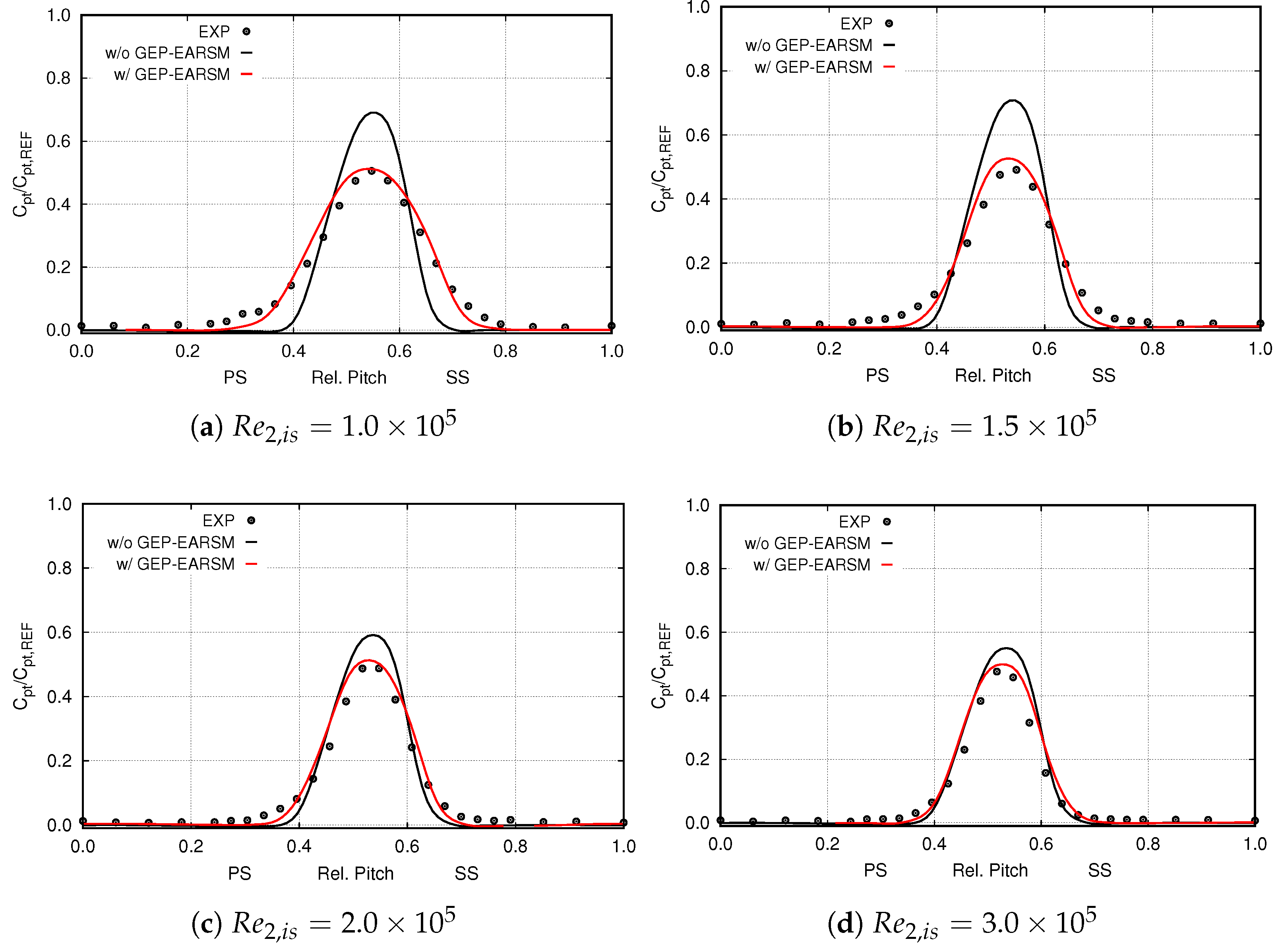
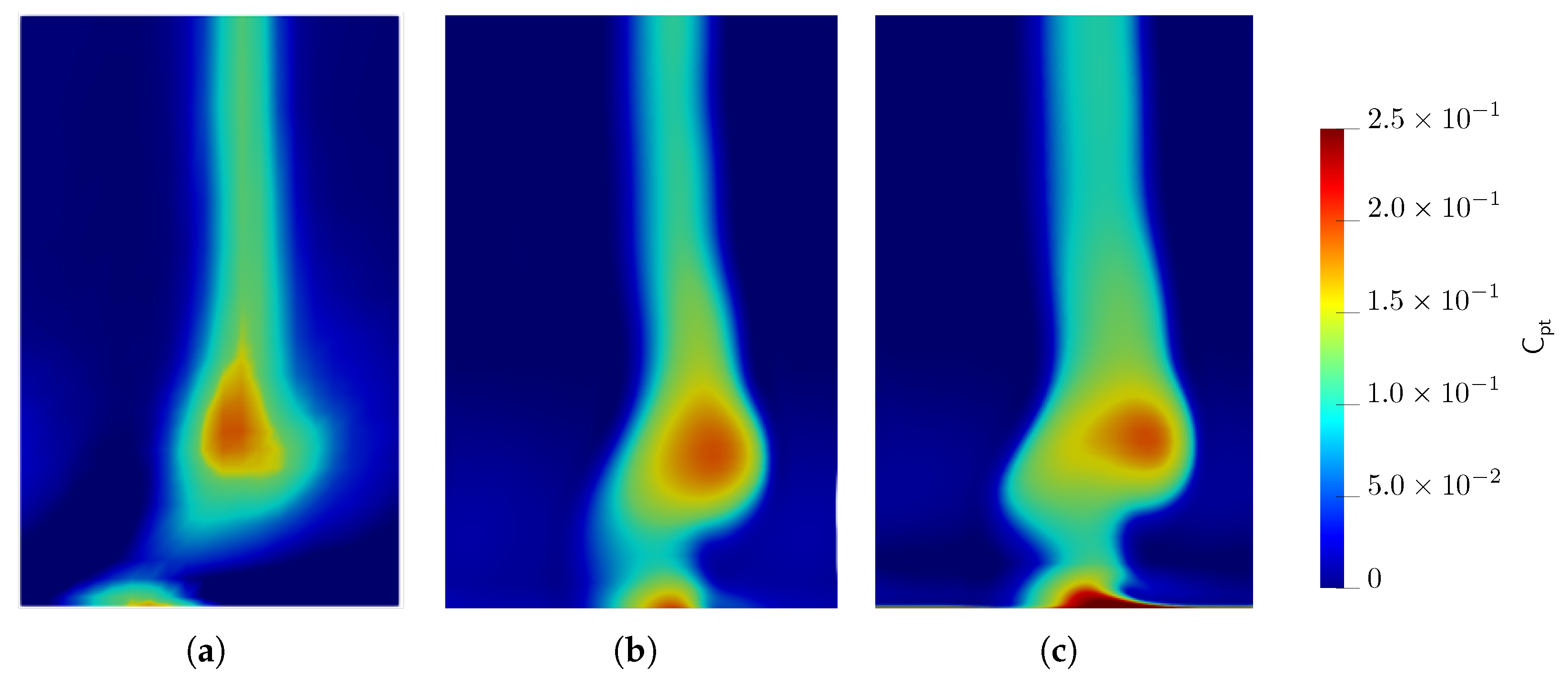
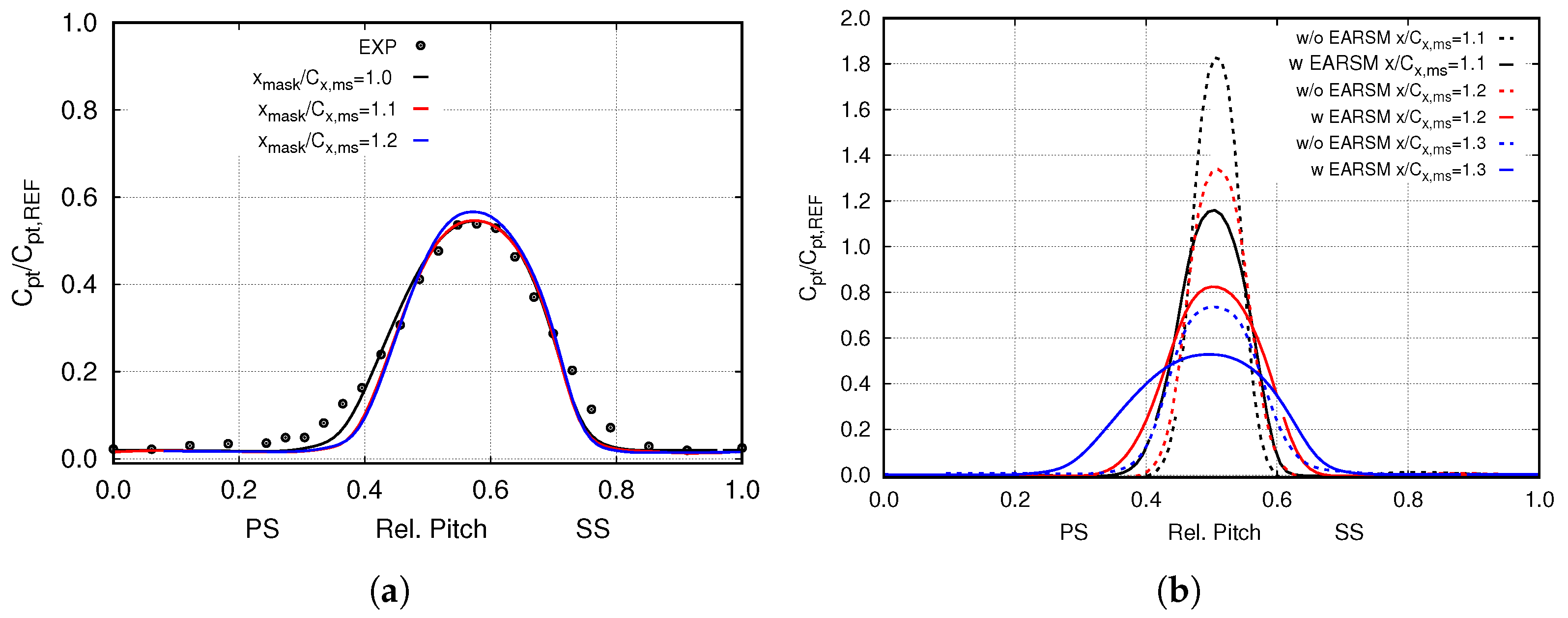
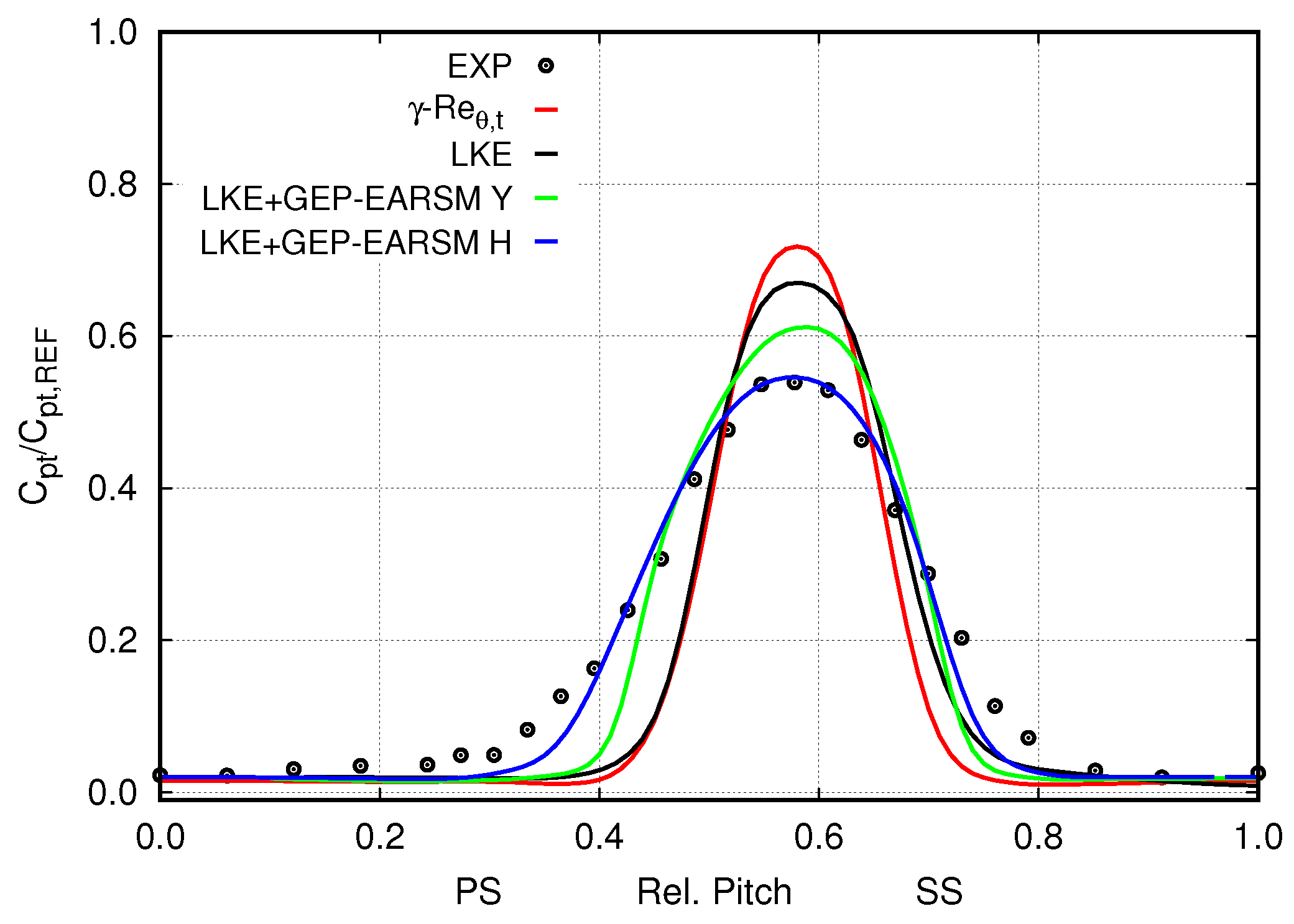
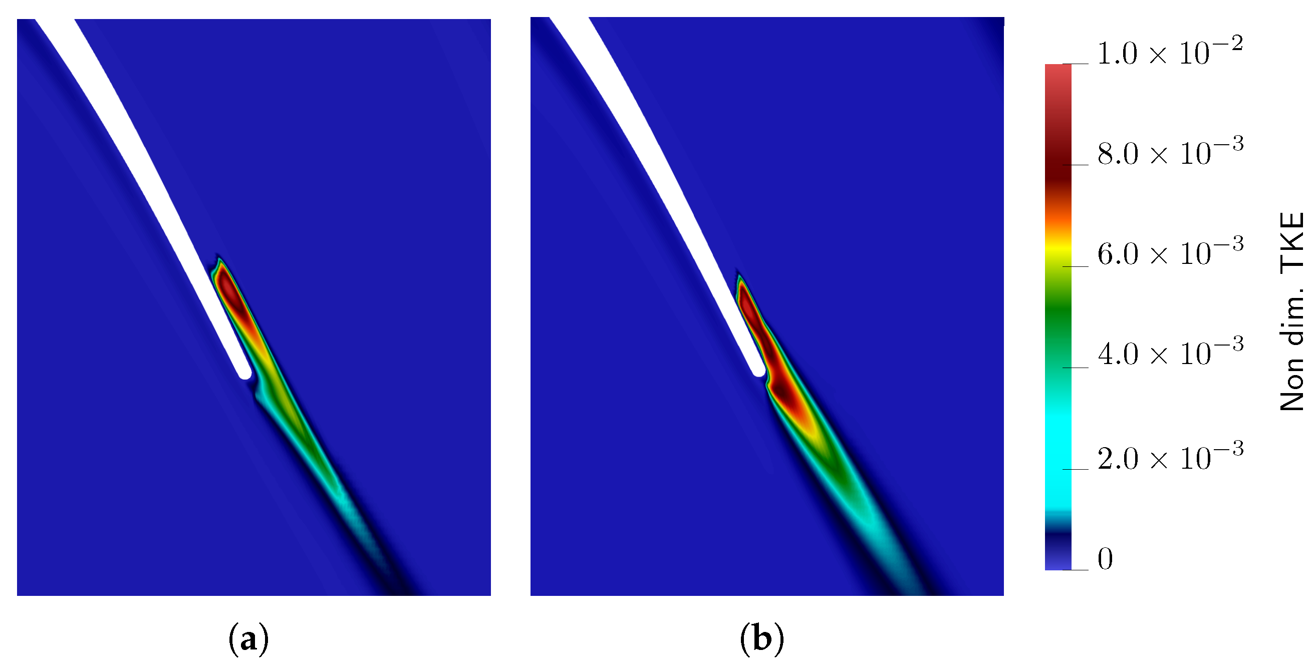
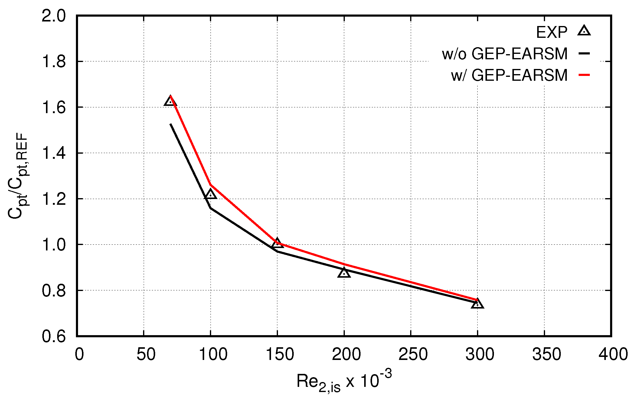
5.2. Wake Diffusion and Effect of the EARSMs

The wake loss profiles generated by the two EARSMs are compared to measurements and to the predictions obtained by the baseline frameworks in Figure 5b. The wake loss profile is reported in terms of total pressure loss coefficient, defined as:

$$C_{pt}=\frac{p_{01}-p_0\left(\overline{y}\right)}{p_{01}-p_2}$$

(9)

where $p_0\left(\overline{y}\right)$ is the local total pressure value as a function of the normalized pitchwise coordinate $\overline{y}=y/g$, along the axial section at $x/C_{x,ms}=1.46$. The total pressure loss coefficient distributions were scaled with a reference $C_{pt}$ value, assumed equal to the measured, tangentially mass averaged, value at $R{e}_{2,is}=1.5\times {10}^5$. The reported results refer to the lowest Reynolds number ($R{e}_{2,is}=0.7\times {10}^5$), where major wake diffusion effects, driven by the relevant suction side separation bubble, are expected.

Despite the highlighted differences in the predicted blade boundary layer structures, there is no significant difference between the baseline model predictions obtained with the $\gamma -R{e}_{\theta ,t}$ and LKE models. They both predict narrower and deeper wake loss profiles as compared to experiments, with a slightly better performance of the LKE model. The application of the GEP-based EARSMs considerably improves the predictions of the wake loss profiles, especially in terms of loss peak reduction. The most remarkable agreement with experimental data is achieved with the GEP-EARSM H, probably due to the fact that such a model was trained on LPT wake flows, in a range of Reynolds number similar to the one considered here. With such a model, the wake centerline loss peak is almost perfectly predicted, and the width, as well as the shape, of the captured wake profile appears correct. Discrepancies in measurements are visible in the peripheral regions of the wake, resulting in a slight underestimation of its tangential extent. Such a behavior of the model was already noticed during the training process [17].

The GEP-EARSM Y calculation still lacks wake diffusion as witnessed by the higher centerline peak and the insufficient wake spreading relative to the measurements. This could appear surprising since the model coefficient for $V_{ij}^{\left(1\right)}$ is larger for the GEP-EARSM Y as compared to the GEP-EARSM H; however, the value of the invariant $I_1$ may offset the coefficient magnitude, and the coefficients for $V_{ij}^{\left(2\right)}$ and $V_{ij}^{\left(3\right)}$ may contribute as well. Moreover, the predicted loss profile is asymmetric, a feature which is not evidenced in the experimental data. On the basis of the discussed results, it was apparent that, between the two considered Reynolds stress closures, the GEP-EARSM H is the best-performing one, and thus only the results obtained with this model are reported in the following.

The results presented in Figure 6 were obtained by applying the machine-learned closures in the wake region starting from the blade trailing edge. As mentioned in the Introduction section, the models were generated with reference to the far wake so that the training process is not biased by the deterministic unsteadiness associated with vortex shedding developing at the trailing edge. As a consequence, their application in the near wake can be questionable, and there was the suspicion it may lead to unphysical results. Actually, flow unsteadiness is not resolved in a RANS approach, and differences in the structure of the near and far wake can hardly be defined. As noticed before, the definition of an automated zonal approach for the application of GEP-based EARMs would be greatly simplified if no distinction between the near and the far wake is made; therefore, with this goal in mind, a sensitivity analysis to the starting axial coordinate of the machine-learned closure application region $x_{mask}$ was carried out. The results of such a study are summarized in Figure 5a that compares tangential $C_{pt}$ distributions computed with $x_{mask}/C_{x,ms}=1.0,1.1$, and $1.2$ with experimental data, at $R{e}_{2,is}=0.7\times {10}^5$. The reported predictions are actually very similar one to the other, and the one with $x_{mask}/C_{x,ms}=1.0$ actually yields the best agreement with measurements. As the activation section is moved downstream, the wake width tends to become underestimated as it can be appreciated in Figure 5a starting from $x_{mask}/C_{x,ms}=1.1$, and, for $x_{mask}/C_{x,ms}=1.2$, a slight discrepancy appears in the centerline loss peak too. Such considerations justify the adopted strategy of applying the machine-learned closures starting from the trailing edge, but, in order to gain more insights into the calculated wake development, comparisons between tangential distributions of $C_{pt}$ obtained with and without the GEP-EARSM H, are reported in Figure 5b in three different axial locations downstream of the blade trailing edge. They correspond to $x/L_{C_{x,ms}}=1.1,1.2,$ and $1.3$, respectively. The application of the GEP-based EARSM produces the largest centerline peak reduction in the first $10\%$ axial chord downstream of the blade TE, indicating that the model actually mimics the breakdown of flow instabilities that occur in this region through increased diffusion. Such an observation is consistent with the nondimensional turbulent kinetic energy contours reported in Figure 7a,b. As a result of the strong anisotropy developing in the trailing edge region, the near wake in the calculation with the GEP-EARSM (Figure 7b) is characterized by a wider region of high TKE relative to the prediction with the baseline model (Figure 7a). As can be seen in Figure 5b, the difference in the loss peak tends to decrease in the following locations, but increased wake diffusion can be observed when moving downstream. In fact, the largest difference in the wake spreading is recorded at $x/C_{x,ms}=1.3$, although it is quite relevant already at $x/C_{x,ms}=1.2$.

A very similar behavior was previously observed in [4], when comparing wake loss profiles predicted with a RANS approach to those obtained from an LES calculation on a three-dimensional cascade based on the T106 blade section.

Figure 8a–d reports the comparison between calculated tangential $C_{pt}$ distributions at $x/C_{x,ms}=1.46$ and experimental data for $R{e}_{2,is}=1.0\times {10}^5$, $1.5\times {10}^5$, $2.0\times {10}^5$, and $3.0\times {10}^5$. The wake-mixing level predicted by the baseline model appears too small at the lowest Reynolds numbers but tends to become more and more correctly reproduced as $R{e}_{2,is}$ increases. For instance, at $R{e}_{2,is}$ (Figure 8a), the computed wake loss profiles appear off both in terms of centerline peak and tangential extent, while at $R{e}_{2,is}$, the $C_{pt}$ tangential distribution appears only mildly too deep. Instead, the wake loss profile computed by the GEP-EARSM are in very good agreement with experiments for all the reported Reynolds number conditions. At low Reynolds numbers, the turbulence anisotropy brought about by the large separation bubble promotes the wake mixing, and such an effect is introduced in the simulation by the GEP-EARSM, while it is not captured by the baseline model. At higher Reynolds numbers, the size of the suction side separation bubble decreases, and this mechanism is attenuated. In the GEP-EARSM calculation, small differences with measurements are visible only in the wake peripheral regions, and they are comparable to those evidenced and discussed for $R{e}_{2,is}=0.7\times {10}^5$ (Figure 5b). Although associated with minor discrepancies, this circumstance evidences a weakness of the model. The computed cascade lapse rates are compared to experiments in Figure 9 in terms of total pressure loss coefficient as a function of the exit isentropic Reynolds number in the downstream section at $x/C_{x,ms}=1.46$ at midspan. The total pressure loss coefficients are again scaled with the reference $C_{pt}$ value. The baseline model reasonably agrees with measurements at the higher Reynolds numbers, up to $R{e}_{2,is}=1.5\times {10}^5$, but underestimates losses at the lowest ones. The larger discrepancy is recorded for $R{e}_{2,is}=0.7\times {10}^5$. The GEP-EARSM model substantially improves the predictions below $R{e}_{2,is}=1.5\times {10}^5$ consistently with a better capturing of the wake-mixing phenomenon.

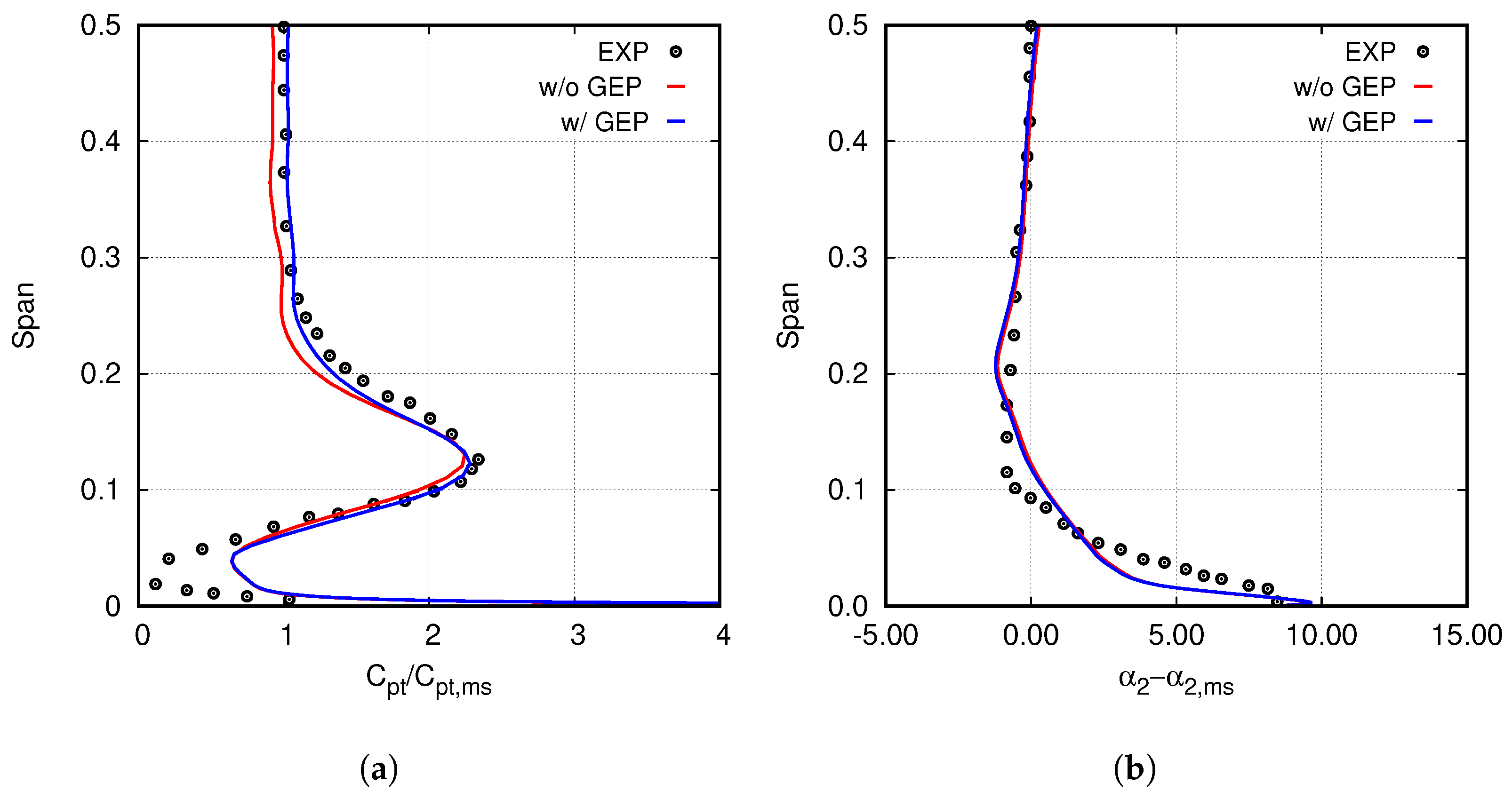
5.3. Secondary Flows

As previously mentioned, the present work was focused on the prediction of wake mixing, but it was interested in assessing how the use of the GEP-EARSM could impact the cascade secondary flow reproduction. This can contribute to the guidelines for constructing a suitable sensing function for the zonal application of the GEP-EARSMs.

The computed spanwise distributions of total pressure loss coefficient and blade-to-blade flow angle in the downstream section at $x/C_{x,ms}=1.46$, for an intermediate value of the Reynolds number ($R{e}_{2,is}=1.5\times {10}^5$), are compared to experiments in Figure 10a,b respectively. The flow angle distribution is presented in terms of deviation with respect to the midspan angle value, while the total pressure coefficient distribution was scaled with the reference value. The total pressure loss coefficient was evaluated as:

$$C_{pt}\left(\overline{z}\right)=\frac{p_{01}\left(\overline{z}\right)-p_{02}\left(\overline{z}\right)}{p_{01}\left(\overline{z}\right)-p_2}$$

(10)

where $\overline{z}=z/h$ is the normalized spanwise coordinate, $p_{01}\left(\overline{z}\right)$ and $p_{02}\left(\overline{z}\right)$ are tangentially mass-averaged total pressure values, at inlet and outlet sections, respectively.

The predictions with and without GEP-EARSM are very similar in terms of loss coefficient distribution. A slight difference is detected in the loss peak at $12\%$ of the span. The shift in the two computed distributions in the core flow (between $20\%$ and $50\%$ of the span) is consistent with the different wake mixing and loss detected by the two models, which lead to different values of the profile loss as reported in Figure 9. The agreement with the experimental data is satisfactory, except for the first $10\%$ of the blade span, where the predictions overestimate the total pressure loss coefficient. In terms of exit flow angles, the computed spanwise distributions are practically coincident and in quite good agreement with experiments.

The tangential distributions of loss coefficient and flow angle would evidence no significant impact on the cascade secondary flow characteristics, but the two-dimensional maps of total pressure loss coefficient actually reveal a somewhat different situation. The experimental, computed without GEP-EARSM, and with GEP-EARSM total pressure loss coefficient contours, taken in the downstream section at $x/C_{x,ms}=1.46$ at $R{e}_{2,is}=1.5\times {10}^5$, are reported in Figure 11a–c.

The predicted shape and location of the main loss core agree quite well with the experimental ones (Figure 11a) for the calculation without the GEP-EARSM (Figure 11b). Instead, the calculation with the GEP-EARSM (Figure 11c) reports a much diffused loss pattern, with a tangential extent of the region affected by secondary flows sensibly larger than the experimental one, and with a smaller loss core. The corner vortex close to the endwall is predicted in a different tangential location relative to measurements by both the simulations. Predictions with and without the application of the GEP-EARSM compare similarly at all the other investigated Reynolds numbers, for which experimental measurements along the span were not available.

Although the adoption of the GEP-EARSM does not impair the secondary flow reproduction on a tangentially averaged sense (Figure 10a,b), the local differences evidenced by the total pressure coefficient contours could have an impact on the interaction with a downstream blade row. This suggests that a sensing function devised to hide the secondary flow affected regions to models trained for wake mixing could be desirable.

6. Conclusions

A three-dimensional cascade representative of state-of-the art LPT bladings was studied using a RANS approach in order to assess the improvement in wake-mixing predictions provided by machine-learned turbulence closures explicitly trained for such a task. The analysis covered several Reynolds number values, in the typical range of operation of LPTs for aeroengine applications, and, in such a range, transition was found to occur due to separated flow. To ensure that the wake originates from correctly reproduced blade boundary-layers, preliminary analyses were carried out to check for the impact of transition closures, coupled with the Wilcox $k-\omega$ model, in the prediction of blade loading distributions. Comparisons with experiments showed that the most accurate predictions are achieved with the LKE model proposed in [30]. In fact, in this case, the relative differences between computed and measured results amount to less than $1\%$.

Two GEP-based EARSMs, namely the ones proposed in [16,17], were considered in the present work. They were applied in a prescribed region downstream the blade trailing edge, excluding the endwall boundary layers. Despite the models having been trained in the far wake, a sensitivity analysis showed that the distance from the trailing edge where they are activated does not impact substantially the predicted results, even if the best performance is obtained when the closures are activated directly at the trailing edge. In this condition, the increased diffusion provided by the model ensures a realistic representation of the wake evolution. These findings also provide a guideline for the construction of a sensing function for the automated application of machine-learned models trained for wake-mixing. The fact that a distinction between near and far wake is not necessary for the application of the closures greatly facilitates their construction.

The most accurate results in terms of wake loss profiles were provided by the model proposed in [17]. The comparison with measured tangential distributions of total pressure loss coefficient demonstrated how the use of such a model results in a substantial improvement in wake mixing and integrated loss predictions over the whole considered Reynolds number range. This qualifies machine-learned closures as a very attractive means not only to achieve more realistic aerodynamic simulations of a single blade row but also for the prediction of the carry-over effect on following blade rows, a feature that paves the way for accurate unsteady rotor–stator interaction analyses using URANS approaches. Discrepancies with measurements are still present in the peripheral region of the wake. In relative terms, they amount to about the $1\%$, and thus, they can be regarded as acceptable for the majority of applications; regardless, they witness scope for improvements in the training of the machine-learned closure.

Finally, the results concerning the cascade secondary flows showed how the GEP-based ERASMs impact the prediction of their structure only on a local basis, slightly worsening its reproduction relative to the baseline model, but without significant changes in the spanwise distributions of tangentially averaged flow quantities. This would suggest that secondary vortices should be masked by a properly defined sensing function in order to be unaffected by machine-learned models trained for wake mixing. The current way of applying the closures in manually prescribed regions of the flow-field could severely limit their use in the analysis of multistage environment, and for this purpose, the highlights for the definition of a sensing function depicted in this paper represent another important result.

References

1. Intergovernmental Panel on Climate Change (IPCC). Global Warming of 1.5 °C, Summary for Policymakers. In Climate Change and Land: An IPCC Special Report on Climate Change, Desertification, Land Degradation, Sustainable Land Management, Food Security, and Greenhouse Gas Fluxes in Terrestrial Ecosystems; IPCC: Geneva, Switzerland, 2019. [Google Scholar]
2. Michelassi, V.; Chen, L.W.; Pichler, R.; Sandberg, R.D. Compressible Direct Numerical Simulation of Low-Pressure Turbines: Part II - Effect of Inflow Disturbances. J. Turbomach. 2015, 137, 071005. [Google Scholar] [CrossRef]
3. Praisner, T.J.; Clark, J.P.; Nash, T.C.; Rice, M.J.; Grover, E.A. Performance Impacts Due to Wake Mixing in Axial-Flow Turbomachinery. In Proceedings of the ASME Turbo Expo, Barcelona, Spain, 8–11 May 2006. ASME paper GT2006-90666. [Google Scholar]
4. Marconcini, M.; Pacciani, R.; Arnone, A.; Michelassi, V.; Pichler, R.; Zhao, Y.; Sandberg, R. Large Eddy Simulation and RANS Analysis of the End-Wall Flow in a Linear Low-Pressure-Turbine Cascade—Part II: Loss Generation. J. Turbomach. 2019, 141, 051004. [Google Scholar] [CrossRef]
5. Hodson, H.P.; Howell, R.J. The Role of Transition in High-Lift Low-Pressure Turbines for Aeroengines. Prog. Aerosp. Sci. 2005, 41, 419–454. [Google Scholar] [CrossRef]
6. Uzol, O.; Zhang, X.F.; Cranstone, A.; Hodson, H.P. Investigation of Unsteady Wake-Separated Boundary Layer Interaction Using Particle-Image-Velocimetry. In Proceedings of the ASME Turbo Expo, Montreal, QC, Canada, 14–17 May 2007. ASME paper No. GT2007-28099. [Google Scholar]
7. Moreau, S. Turbomachinery Noise Predictions: Present and Future. Acoustics 2019, 1, 92–116. [Google Scholar] [CrossRef] [Green Version]
8. Burberi, C.; Ghignoni, E.; Pinelli, L.; Marconcini, M. Validation of an URANS approach for direct and indirect noise assessment in a high pressure turbine stage. Energy Procedia 2018, 148, 130–137. [Google Scholar] [CrossRef]
9. Pinelli, L.; Poli, F.; Marconcini, M.; Arnone, A.; Spano, E.; Torzo, D. Validation of a 3D Linearized Method for Turbomachinery Tone Noise Analysis. In Proceedings of the ASME Turbo Expo, Vancouver, BC, Canada, 6–10 June 2011. ASME paper GT2011-45886. [Google Scholar]
10. Pacciani, R.; Marconcini, M.; Arnone, A.; Bertini, F. A CFD Study of Low Reynolds Number Flow in High Lift Cascades. In Proceedings of the ASME Turbo Expo, Glasgow, UK, 14–18 June 2010. ASME paper GT2010-23300. [Google Scholar]
11. Duraisamy, K.; Iaccarino, G.; Xiao, H. Turbulence Modeling in the Age of Data. Annu. Rev. Fluid Mech. 2019, 53, 357–377. [Google Scholar] [CrossRef] [Green Version]
12. Weatheritt, J.; Sandberg, R.D. The development of algebraic stress models using a novel evolutionary algorithm. Int. J. Heat Fluid Flow 2017, 68, 298–318. [Google Scholar] [CrossRef]
13. Ferreira, C. Gene Expression Programming: A New Adaptive Algorithm for Solving Problems. Complex Syst. 2001, 13, 87–129. [Google Scholar]
14. Akolekar, H.D.; Weatheritt, J.; Hutchins, N.; Sandberg, R.D.; Laskowski, G.; Michelassi, V. Development and Use of Machine-Learnt Algebraic Reynolds Stress Models for Enhanced Prediction of Wake Mixing in Low Pressure Turbines. J. Turbomach. 2019, 141, 041010. [Google Scholar] [CrossRef]
15. Akolekar, H.D.; Sandberg, R.D.; Hutchins, N.; Michelassi, V.; Laskowski, G. Machine-Learnt Turbulence Closures for Low Pressure Turbines with Unsteady Inflow Conditions. J. Turbomach. 2019, 141, 101009. [Google Scholar] [CrossRef]
16. Zhao, Y.; Akolekar, H.D.; Weatheritt, J.; Michelassi, V.; Sandberg, R.D. RANS Turbulence Model Development using CFD-Driven Machine Learning. J. Comput. Phisycs 2020, 411, 109413. [Google Scholar] [CrossRef] [Green Version]
17. Akolekar, H.; Zhao, Y.; Sandberg, R.D.; Pacciani, R. Integration of Machine Learning and Computational Fluid Dynamics to Develop Turbulence Models for Improved Low-Pressure Turbine Wake Mixing. J. Turbomach. 2021, 143, 121001. [Google Scholar] [CrossRef]
18. Lav, C.; Sandberg, R.D.; Philip, J. A Framework to Develop Data-Driven Turbulence Models for Flows with Organised Unsteadiness. J. Comput. Phisycs 2019, 383, 148–165. [Google Scholar] [CrossRef]
19. Langtry, R.B.; Menter, F.R. Correlation-Based Transition Modeling for Unstructured Parallelized Computational Fluid Dynamics Codes. AIAA J. 2009, 47, 2894–2906. [Google Scholar] [CrossRef]
20. Pacciani, R.; Marconcini, M.; Fadai-Ghotbi, A.; Lardeau, S.; Leschziner, M.A. Calculation of High-Lift Cascades in Low Pressure Turbine Conditions Using a Three-Equation Model. J. Turbomach. 2011, 133, 031016. [Google Scholar] [CrossRef]
21. Wilcox, D.C. Multiscale Model for Turbulent Flows. AIAA J. 1988, 26, 1311–1320. [Google Scholar] [CrossRef]
22. Simoni, D.; Berrino, M.; Ubaldi, M.; Zunino, P.; Bertini, F. Off-Design Performance of a Highly Loaded LP Turbine Cascade Under Steady and Unsteady Incoming Flow Conditions. J. Turbomach. 2015, 137, 071009. [Google Scholar] [CrossRef]
23. Marconcini, M.; Pacciani, R.; Arnone, A.; Bertini, F. Low-Pressure Turbine Cascade Performance Calculations with Incidence Variation and Periodic Unsteady Inflow Conditions. In Proceedings of the ASME Turbo Expo, Montreal, QC, Canada, 15–19 June 2015. ASME paper GT2015-42276. [Google Scholar]
24. Giovannini, M.; Rubechini, F.; Marconcini, M.; Simoni, D.; Yepmo, V.; Bertini, F. Secondary Flows in Low- Pressure Turbines Cascades: Numerical and Experimental Investigation of the Impact of the Inner Part of the Boundary Layer. J. Turbomach. 2018, 140, 111002. [Google Scholar] [CrossRef]
25. Pichler, R.; Zhao, Y.; Sandberg, R.; Michelassi, V.; Pacciani, R.; Marconcini, M.; Arnone, A. Large-Eddy Simulation and RANS Analysis of the End-Wall Flow in a Linear Low-Pressure Turbine Cascade, Part I: Flow and Secondary Vorticity Fields Under Varying Inlet Condition. J. Turbomach. 2019, 141, 121005. [Google Scholar] [CrossRef]
26. Ricci, M.; Pacciani, R.; Marconcini, M.; Arnone, A. Prediction of Tip Leakage Vortex Dynamics in an Axial Compressor Cascade Using RANS Analyses. In Proceedings of the ASME Turbo Expo, London, UK, 22–26 June 2020. ASME paper GT2020-14797. [Google Scholar]
27. Arnone, A. Viscous Analysis of Three–Dimensional Rotor Flow Using a Multigrid Method. J. Turbomach. 1994, 116, 435–445. [Google Scholar] [CrossRef]
28. Chorin, A.J. A Numerical Method for Solving Incompressible Viscous Flow Problems. J. Comput. Phys. 1967, 2, 12–26. [Google Scholar] [CrossRef]
29. Pacciani, R.; Marconcini, M.; Arnone, A. Comparison of the AUSM+-up and Other Advection Schemes for Turbomachinery Applications. Shock Waves 2019, 29, 705–716. [Google Scholar] [CrossRef]
30. Pacciani, R.; Marconcini, M.; Arnone, A.; Bertini, F. An Assessment of the Laminar Kinetic Energy Concept for the Prediction of High-Lift, Low-Reynolds Number Cascade Flows. Proc. Inst. Mech. E Part A J. Power Energy 2011, 225, 995–1003. [Google Scholar] [CrossRef]
31. Pacciani, R.; Marconcini, M.; Arnone, A.; Bertini, F. Predicting High-Lift LP Turbine Cascades Flows Using Transition-Sensitive Turbulence Closures. J. Turbomach. 2014, 136, 051007. [Google Scholar] [CrossRef]
32. Pope, S.B. A More General Effective-Viscosity Hypothesis. J. Fluid Mech. 1975, 72, 331–340. [Google Scholar] [CrossRef] [Green Version]
Figure 1. Sketch of the test rig.
Energies 14 08327 g001
Figure 2. Inlet boundary layer total pressure profile.
Energies 14 08327 g002
Figure 3. Blade surface distributions of (a) pressure-coefficient (b) skin friction ( R e 2 , i s = 3.0 × 10 5 ).
Energies 14 08327 g003
Figure 4. Blade surface distributions (a) pressure-coefficient (b) skin friction ( R e 2 , i s = 0.7 × 10 5 ).
Energies 14 08327 g004
Figure 5. Wake loss profiles at R e 2 , i s = 0.7 × 10 5 , (a) obtained with different values of x m a s k (GEP-EARSM, x / C x , m s = 1.46 ), (b) in different locations downstream of blade TE (GEP-EARSM H).
Energies 14 08327 g005
Figure 6. Wake loss profiles w/ and w/o GEP-EARSM ( R e 2 , i s = 0.7 × 10 5 , x / C x , m s = 1.46 ).
Energies 14 08327 g006
Figure 7. Nondimensional turbulent kinetic energy at midspan (a) without GEP-EARSM (b) with GEP-EARSM ( R e 2 , i s = 0.7 × 10 5 ).
Energies 14 08327 g007
Figure 8. Wake loss profiles ( x / C x , m s = 1.46 ).
Energies 14 08327 g008
Figure 9. Cascade lapse rate (midspan losses, x / C x , m s = 1.46 ).
Energies 14 08327 g009
Figure 10. Spanwise distribution of (a) total pressure loss coefficient (b) blade-to-blade flow angle ( R e 2 , i s = 1.5 × 10 5 , x / C x , m s = 1.46 ).
Energies 14 08327 g010
Figure 11. Contours of total pressure loss coefficient (a) Experimental (b) without GEP-EARSM (c) with GEP-EARSM.
Energies 14 08327 g011