Transition Modeling for Low Pressure Turbines Using Computational Fluid Dynamics Driven Machine Learning

Abstract

Existing Reynolds Averaged Navier–Stokes-based transition models do not accurately predict separation induced transition for low pressure turbines. Therefore, in this paper, a novel framework based on computational fluids dynamics (CFD) driven machine learning coupled with multi-expression and multi-objective optimization is explored to develop models which can improve the transition prediction for the T106A low pressure turbine at an isentropic exit Reynolds number of $R{e}_{2is}=100,000$. Model formulations are proposed for the transfer and laminar eddy viscosity terms of the laminar kinetic energy transition model using seven non-dimensional pi groups. The multi-objective optimization approach makes use of cost functions based on the suction-side wall-shear stress and the pressure coefficient. A family of solutions is thus developed, whose performance is assessed using Pareto analysis and in terms of physical characteristics of separated-flow transition. Two models are found which bring the wall-shear stress profile in the separated region at least two times closer to the reference high-fidelity data than the baseline transition model. As these models are able to accurately predict the flow coming off the blade trailing edge, they are also able to significantly enhance the wake-mixing prediction over the baseline model. This is the first known study which makes use of ‘CFD-driven’ machine learning to enhance the transition prediction for a non-canonical flow.

1. Introduction

As air travel is predicted to see continued growth, the aviation industry is focused on further improving the efficiency of gas turbines. Any technological advances which incrementally increase gas turbine efficiency can save millions of dollars, reduce carbon emissions, and create a sustainable future. One place to bring about such a change is at the grassroots level of engine component design by understanding and enhancing the ability to model the flow physics of these components in an increasingly holistic, yet cheaper manner.

Low-pressure turbines (LPT) are one of the most important components which drive the efficiency of gas turbines. If the efficiency of the LPT increases by 1%, the specific fuel consumption will decrease by 0.6–0.8% [1], translating into considerable fuel savings and emissions reductions, considering the volume of operations. LPT design and analysis is challenging as there is a large variation in flow physics between the aircraft taking off and entering cruise conditions. The Reynolds number of LPTs ranges from 0.5 × 10${}^5$ at cruise to 5 ×${10}^5$ at takeoff [2]. This causes a change in the boundary layers from turbulent at takeoff to transitional at cruise, which is the major portion of the flight. At lower Reynolds numbers (cruise), boundary-layer transition and separation play an important role in determining engine performance. There are three modes of transition: natural, bypass and separated-flow [3]. In LPTs, bypass and separated-flow transitions are the most common transition modes. Natural transition begins with weak instabilities in the laminar boundary layer, which lead to three-dimensional instabilities resulting in turbulent spots [4]. However, when free-stream turbulence intensities are greater than 1%, boundary layers typically proceed from laminar to fully turbulent states without the occurrence of linear instabilities, thus bypassing various stages of natural transition. This is called bypass transition. Transition may also occur in the free shear-layer flow that results when a laminar boundary layer separates. The flow could reattach and form a laminar-separation/turbulent-reattachment bubble or could remain detached resulting in an open separation. Separated-flow transition occurs in regions of adverse pressure gradients near the leading edge or after peak suction in LPTs. Separated-flow transition also plays an important role in periodic unsteady transition wherein unsteady incoming wakes from previous blade rows interact with the separation bubble on the LPT suction-side [5]. Separated boundary layers with longer separation bubbles produce greater loss and cause larger deviation in exit flow angles [6], and they are thus to be avoided. At low Reynolds numbers, transition controls the extent of the separation bubble and a reliable prediction of these aspects is crucial for the design of blades with high-lift.

With the increase of computational power, high-fidelity simulations [1,7] that are able to accurately predict the transition phenomena have become feasible. However, they are still not viable as an iterative industrial design tool, due to the associated high cost. Thus, industry remains quite heavily dependent on RANS (Reynolds Averaged Navier–Stokes) calculations as they are a cost-effective way of modeling turbulent flows for engineering solutions. Several transition models are at the disposal of turbomachinery designers [8]. The $\gamma -R{e}_{\theta }$ model [9] uses two transport equations for the intermittency ($\gamma$) and transition momentum thickness Reynolds number (Re${}_{\theta }$), in addition to the turbulent kinetic energy (TKE) and specific dissipation. A class of models uses the laminar kinetic energy (LKE) concept [10,11], wherein an additional transport equation is solved for the LKE. The k${\overline{v}}_2\omega$ model solves an additional transport equation for ${\overline{v}}_2$, which represents wall-normal velocity fluctuations responsible for transition initiation. However, all of these existing RANS-based transition models struggle to accurately predict the onset and extent of separation on the suction-side of the aft portion of the LPT blade. Therefore, novel methods and models have to be explored in order to enhance the accuracy of transition prediction in the context of RANS.

Data-driven turbulence modeling is a field that has gained tremendous momentum in recent years [12]. In fact, many leading researchers [13,14,15] view data-driven turbulence modeling as a promising avenue for bridging the gap between the accuracy of high and low fidelity simulations, while maintaining the same order of cost as low-fidelity calculations. With the help of machine learning processes, high-fidelity datasets can be harvested to extract meaningful physics-based insights to improve the accuracy of RANS calculations. Many different data-driven approaches have been applied to a large variety of industrially relevant cases. Neural networks embedding Galilean invariance to modify the anisotropy tensor were proposed by Ling et al. [16]. With these neural networks, they improved the Reynolds stress and velocity field predictions over linear eddy viscosity models for duct flows and flow over wavy walls. Milani et al. [17] extended the work of Ling et al. [16] and developed a deep neural network to model the scalar-flux of turbulent diffusivity for two different jets in crossflow. Milani et al. [18,19] also used random forests to improve heat-flux modeling for film cooling applications. A more comprehensive overview of existing data-driven methods for turbulence model development can be found in [12,20,21].

It is evident that neural networks are the most popular way to improve the Reynolds stress and mean flow prediction. However, one major drawback lies in their ‘black box’ nature—they are difficult to interpret as physics-based information remains hidden in the network. An alternative that addresses this issue is symbolic regression, which produces interpretable and explicit model forms. Ferreria [22] introduced gene expression programming (GEP) which was a new evolutionary algorithm for solving regression based problems. Weatheritt and Sandberg [23] developed GEP for turbulence modeling, which creates Galilean invariant turbulence closures, also known as explicit algebraic Reynolds stress models (EARSM). The GEP algorithm for turbulence model development produces tangible symbolic expressions which can be correlated to physical phenomena and can be directly inserted into RANS codes. For example, Akolekar et al. [24] correlated different models from GEP to physical mechanisms such as laminar separation and wake–wake interactions in LPTs with unsteady inflow conditions using a zonal model development approach.

GEP also offers the added advantage of less computational cost over neural networks, in both the development and implementation phases. GEP has been successfully applied to a number of canonical and industrial (complex flows) turbulence modeling problems by enhancing the flow prediction capability for RANS and LES. Akolekar et al. [25] developed EARSMs for enhancing the prediction of LPT wake flow originating from open and closed separated boundary layers using ‘frozen’ [26] high-fidelity databases (the ‘frozen’ methodology only solves the RANS equations for those quantities which cannot be directly obtained from a high-fidelity database—for example, the specific dissipation rate ($\omega$) is not readily available from a high-fidelity database and is thus derived from a RANS calculation while keeping all other values constant—i.e., as derived from high-fidelity calculations). They also tested these EARSMs successfully on high-pressure turbine (HPT) flows [27], thus demonstrating the robustness of the models developed. Weatheritt et al. [28] developed GEP-based EARSMs for HPTs and assessed their performance in an a priori sense. Recently, Zhao et al. [29] introduced a novel ‘CFD-driven’ (computational fluid dynamics) framework for turbulence model development based on GEP. This algorithm uses RANS feedback as part of the model training process. It was found that this method has high potential for offering robust turbulence closures to enhance the wake mixing prediction across different high and low pressure turbine operating conditions and blade geometries [30]. Waschkowski et al. [31] recently proposed a multi-objective and multi-expression extension to the ‘CFD-driven’ framework. The multi-objective approach makes use of different cost functions simultaneously, whereas the multi-expression capability develops coupled turbulence closures across different regions of the flow field.

Efforts to enhance the accuracy of transition modeling with machine learning have only recently begun. Zafar et al. [32] developed a convolutional neural network based transition model capable of accurately predicting the transition onset location for incompressible, two-dimensional attached flows in a physically informed manner, without requiring direct computations, from linear instability theory. Yang and Xiao [33] developed a framework to improve transition models using field inversion and machine learning for airfoils. There are no studies, however, which focus on enhancing transition prediction of RANS models using machine learning for LPTs. There is thus immense scope to improve the performance of existing RANS models for transition prediction with machine learning techniques. GEP is an ideal algorithm to formulate new transition models as expressions can be formulated which yield physical insights into the modeling process.

This study, therefore, proposes a novel machine learning framework based on GEP to generate models which enhance the prediction of separated-flow transition in LPTs. First, a brief overview of the LKE transition model [11], which is the baseline model used in this study, is presented. The functional forms of the LKE model‘s production and transfer terms are then modified using non-dimensional pi groups [34] based on local flow quantities. An extensive discussion ensues on the scientific ideology of making use of these particular pi groups. Using the recently developed multi-objective cost function based GEP algorithm [31] and the ‘CFD-driven’ [29] framework, models which enhance the separated-flow transition are proposed. The performance of these models is evaluated in terms of Pareto analysis and physical characteristics such as wall-shear stress, blade loading and turbulent wake mixing. This is the first known study which makes use of ‘CFD-driven’ machine learning to enhance the separation-induced transition prediction based on multi-objective and multi-expression optimization using non-dimensional pi groups.

2. Transition Modeling

The LKE transition model [11] is used as the baseline model. This section discusses the transport equations used for the LKE transition model. It also discusses the intricacies of making possible improvements in the LKE model using non-dimensional pi groups.

2.1. Laminar Kinetic Energy Model

This study makes use of a transition model developed by Pacciani et al. [11] which is based on the LKE concept, as introduced by Mayle and Schulz [35], and takes into account the pre-transitional rise of the fluctuating kinetic energy. The modeled transport equation for the LKE $\left(k_l\right)$, with $\nu$ as the kinematic viscosity, is

$$\frac{D{k}_l}{Dt}=P_l-2\nu \frac{k_l}{y^2}+\nu {\nabla }^2{k}_l-R.$$

(1)

The gradual rise of pre-transitional energy in the separated region is modeled using a production term ($P_l$) based on the mean shear rate (S) and a laminar eddy viscosity concept [36]. It is expressed as

$$\begin{array}{cc}\hfill P_l=& {\nu }_l{S}^2,\hfill \\ \hfill {\nu }_l=& C_1{f}_1\sqrt{k_l}{\delta }_{\mathsf{\Omega }},\hfill \\ \hfill f_1\left(Tu\right)=& max\left[0.8,2.0·tanh\left(\left(\frac{Tu}{4.5}\right)\right)\right],\hfill \\ \hfill {\delta }_{\mathsf{\Omega }}=& {max}_y\left(\frac{U}{\mathsf{\Omega }}\right),\hfill \end{array}$$

(2)

where ${\nu }_l$ is the laminar eddy viscosity, $C_1$ = 0.01, $f_1$ is defined as a function of the inlet free-stream turbulence intensity (Tu), ${\delta }_{\mathsf{\Omega }}$ is the maximum in the normal-to-the-wall direction shear-layer vorticity thickness which is assumed as a length scale representative of separated laminar flow and l is a proper length scale, characteristic of the transition mode to be represented (natural, bypass or separated-flow). $\mathsf{\Omega }$ is the vorticity magnitude and U is the magnitude of velocity. The choice of a vorticity-based length scale for the LKE production term was motivated by the fact that the most unstable wavelength in the separated shear-layer is related to the shear-layer thickness. The fluctuating energy is then gradually transferred to the turbulence field via a transfer term (R) which is defined as

$$\begin{array}{cc}\hfill R=& C_2{\beta }^{*}{f}_2\omega k_l,\hfill \\ \hfill f_2=& 1-e^{-\psi /C_3},\hfill \\ \hfill \psi =& max(0,R_y-C_4),\hfill \\ \hfill R_y=& \frac{\sqrt{k}y}{\nu },\hfill \end{array}$$

(3)

with $C_2=0.3$, $C_3=8$, $C_4=10$ and ${\beta }^{*}=0.09$. $f_2$ is a damping function and $R_y$ is the wall distance Reynolds number with y as the wall-normal wall distance. The quantity $\psi$ can be considered as the transition parameter as it controls the transfer of energy from the laminar to the turbulent state, which occurs when the wall distance Reynolds number $R_y$ reaches the threshold value of $C_4$. The term R appears in both laminar and TKE (k) transport equations which indicates no net change in the total fluctuating kinetic energy. This term implies that there is a transfer of energy from $k_l$ to k. The TKE transport equation is written as

$$\frac{Dk}{Dt}=P_k-{\beta }^{*}{f}_{k}k\omega +\frac{\partial }{\partial x_j}\left[(\nu +{\sigma }_k{\nu }_T)\frac{\partial k}{\partial x_j}\right]+R,$$

(4)

where ${\sigma }_k=0.5$ and the TKE production $\left(P_k\right)$ is modeled as

$$P_k={\tau }_{ij}\frac{\partial u_i}{\partial x_j}=f_{\mu }{\nu }_t{S}^2,$$

(5)

where ${\tau }_{ij}$ is the Reynolds stress tensor from the Boussinesq approximation [37], S is the magnitude of the strain-rate tensor and ${\nu }_T$ is the turbulence eddy viscosity. The closure damping functions are

$$f_{\mu }=1-0.975exp\left(\frac{-R{e}_T}{2.5}\right);f_k=1-0.722exp\left[-{\left(\frac{R{e}_T}{4.5}\right)}^4\right],$$

(6)

where $R{e}_T$ is the turbulence Reynolds number and is equal to $k/(\nu \omega )$. The transport equation of the specific dissipation rate is given as

$$\frac{D\omega }{Dt}=\alpha \frac{\omega }{k}{P}_k-\beta {\omega }^2+\frac{\partial }{\partial x_j}\left[(\nu +{\sigma }_{\omega }{\nu }_T)\frac{\partial \omega }{\partial x_j}\right],$$

(7)

with $\alpha =3/40$, $\beta =5/9$ and ${\sigma }_{\omega }=0.5$.

2.2. Proposed Model Formulation

In the LKE transition model, the LKE production ($P_l$) and transfer (R) terms play a crucial role in determining the transition onset and extent. It is proposed in this study to modify certain parts of these terms. The scientific ideology as well as the method of achieving this is discussed below.

2.2.1. Scientific Ideology

The LKE model, with some success, was applied to the prediction of separated-flow transition in LPT cascades by Pacciani et al. [11,38], where the vorticity thickness of the separated shear-layer was assumed as a length scale. However, the eddy viscosity equation (Equation (2)) has two significant drawbacks. Firstly, it involves non-local quantities (e.g., the shear-layer vorticity thickness). Secondly, it does not account for the free-stream turbulence level. This latter deficiency was addressed by introducing the function $f_1$, which is expressed in terms of the inlet free-stream turbulence intensity Tu. Such a modification yielded satisfactory results on isolated cascades, as shown by Pacciani et al. [39]. However, the ${\nu }_l$ term has to consequently be modified in order to include only local quantities.

The transfer term R is formulated following Walters and Cokljat [10]. Equation (3) has proven to be reliable in RANS calculations of separated-flow transition as it results in separation bubble lengths, transition onset locations and pressure recovery prior to reattachment that are in good agreement with experimental data [11,38]. On many accounts, it is observed that the transition onset is dependent on the Reynolds number, pressure gradient and free-stream turbulence intensity. It is therefore argued that the term $R_y-C_4$ in the $\psi$ function is too crude for triggering the transition onset. A better formulation, which is representative of the flow physics, has to be found for $\psi$.

In addition, the LKE model [11] was conceived for separated-flow transition prediction as the adopted length scale is a useful measure of the most unstable Kelvin–Helmholtz (KH) modes. The length scale also bears a loose relation with fluctuations developing in attached boundary-layers (Tollmien–Schlichting waves and Klebanoff streaks). A step forward towards a true LKE-based multi-mode model requires a more general framework that is able to address the growth of pre-transitional fluctuations in attached and separated boundary layers under the effects of the turbulent scales coming from the free-stream. Therefore, we propose the use of non-dimensional pi groups in order to modify certain terms of the LKE model. The use of machine learning (see Section 3) will make the process more efficient and holistic.

2.2.2. Non-Dimensional Pi Groups

The transition problem is based on a number of local independent dimensional variables. In order to best capture the effect of these independent dimensional variables on the dependent variables (for example, the $\psi$ term), the Buckingham pi theorem [34] is used to create dimensionless groups, called pi groups. Seven non-dimensional pi groups are considered as possible input parameters to modify the LKE production term (Equation (2)) and the transfer term (Equation (3)) as

$$\begin{array}{cc}\hfill & {\Pi }_1=\frac{k_l}{\nu \Omega };{\Pi }_2=\frac{\Omega y}{U};{\Pi }_3=\frac{y}{l_t};{\Pi }_4=\frac{\sqrt{k}y}{\nu };\hfill \\ & {\Pi }_5=\frac{k}{\nu \Omega };{\Pi }_6=\frac{Sy}{U};{\Pi }_7=\frac{\omega }{\Omega },\hfill \end{array}$$

(8)

where $\nu$ is the kinematic viscosity and the turbulence length scale is defined as $l_t=\frac{\sqrt{k}}{\omega }$. The particular choice for the pi groups is motivated by their widespread use as transition sensor functions in a variety of models (${\Pi }_4$, ${\Pi }_5$ and ${\Pi }_6$ [8]), by their nature of scale-determining terms for laminar fluctuations (${\Pi }_1$, ${\Pi }_2$ and ${\Pi }_6$) or for turbulent fluctuations coming from the free-stream (${\Pi }_3$ and ${\Pi }_7$). ${\Pi }_1$ can be regarded as the ratio of two time scales: the time scale for the convection of disturbances in the laminar boundary layer ($1/omega$) and the time scale for the diffusion of large-scale fluctuations (e.g., KH instabilities) from the edge of the shear-layer ($k_l/\nu {\omega }^2$). ${\Pi }_2$ and ${\Pi }_6$ are relevant scales for the separated shear-layer thickness with the advantage of being local parameters. In the construction of such groups, the use of the vorticity magnitude in favor of the strain rate appeared somewhat arbitrary. It was therefore decided to include both formulations, letting the machine learning framework determine the respective roles. ${\Pi }_3$ is a scale-determining term for the turbulent fluctuations coming from the edge of the boundary layer. ${\Pi }_4$ is a turbulent Reynolds number based on wall distance. It accounts for the rise of turbulent kinetic energy inside the boundary layer. Its use as a transition onset parameter is extremely common in transition frameworks coupled with $k\omega$ turbulence models [8,9,10]. In this role, it is a fundamental component of the original model formulation and it has proven effective in switching on the transfer term when transition is initiated. ${\Pi }_5$ is a well-established shear-sheltering parameter. Shear-sheltering is the phenomenon by which small-scale, high-frequency, freestream perturbations are damped out by the laminar boundary layer. ${\Pi }_7$ is again the ratio of two time scales, where the laminar fluctuation time scale is now compared with the turbulent time scale ($1/\omega$).

Based on the shortcomings of the LKE model (Section 2.2.1), we propose to modify the laminar eddy viscosity (${\nu }_l$) term from the LKE production term ($P_l$) and the transition parameter ($\psi$) from the transfer term (R) using the non-dimensional pi groups. If a local formulation for ${\nu }_l$ has to be found in terms of non-dimensional pi groups and local flow quantities, it can be represented as

$${\nu }_l=f_{1a}y\sqrt{k_l},$$

(9)

where $f_{1a}=f\left({\Pi }_i\right)$. The machine learning processes in the model development process are tasked to find an expression for $f_{1a}$ based on symbolic regression. There is no restriction on the order or the number of terms in the expression of $f_{1a}$. In order to ensure realizability of the production term, only the terms which ensure $f_1>0$ are selected for model evaluation, which is enforced by a limiter. It was also found that, to keep an upper limit on the value of $f_{1a}$, an additional limiter $min(f_1,f_{1a})$ is also used. This limiter ensures stability and ease of convergence in the calculations. It also ensures that $f_{1a}$ is activated only in the regions of interest, and not everywhere, as is evident in Section 5.2.3.

In its current form, $\psi$ can be represented in terms of the non-dimensional pi groups as $\psi =max({\Pi }_4-C_4,0)$. Initially, an attempt was made to find an expression for $\psi$ without the use of a limiter. However, it was found that it was creating non-physical and unstable solutions in the laminar boundary layer as it was activating the transfer term which should be zero in the laminar boundary layer. Another consideration was to model the entire transfer term (R); however, the machine learning algorithm was not proposing a transfer function which would tend to zero when moving closer towards the wall. A consideration was also made on whether only the LKE production term or transfer term can be modified, without modifying the other one. However, since there is strong coupling between the two terms, both have to be modified together. Therefore, using any linear or non-linear combination of the non-dimensional pi groups, an expression is to be found for

$$\psi =max(f_{2a}\left({\Pi }_i\right),0).$$

(10)

3. Machine Learning Framework

This section discusses the various aspects of the machine learning transition modeling framework. The advantages of the ‘CFD-driven’ algorithm and the extensions by Waschkowski et al. [31] are explained. The methodology of this framework is also elucidated.

3.1. Advantages

GEP-based EARSM development had been centered around the ‘frozen’ approach [24,25] until the integration of CFD with GEP was made by Zhao et al. [29]. The ‘CFD-driven’ approach is feasible with GEP, because the GEP algorithm returns explicit model equations that can be instantly and automatically be implemented into RANS solvers during the model development process. Since RANS calculations are then performed as part of the training loop, the resulting ‘CFD-driven’ models are tested in their target environment and are thus ready to be directly implemented into industrial design tools. Another advantage of the ‘CFD-driven’ training is that the definition of the cost function is more flexible as compared to the ‘frozen’ approach. Rather than being restricted to the quantities that can be directly calculated from the model equations, such as the anisotropy tensor or TKE production, the cost functions used in the ‘CFD-driven’ approach can be tailored to capture any important flow feature of interest. One can specify any mean or secondary statistic profiles in order to derive a suitable model. In fact, if large databases of high-fidelity data are unavailable and only few experimental or high-fidelity profiles are available, this approach has the potential to offer suitable models based on this limited data. This approach also ensures that the models generated are numerically stable as they have already been executed in CFD calculations. This ‘CFD-driven’ framework has so far been successfully applied to turbulence model improvement for wake mixing problems [29,30].

All current machine learning frameworks in the context of data-driven turbulence modeling, including GEP-based model development (both ‘frozen’ and ‘CFD-driven’), are limited to developing one model per training run and only use one cost function (or a single training objective). However, the recent study of Waschkowski et al. [31] introduced multi-expression and multi-objective capabilities as extensions to the ‘CFD-driven’ approach to overcome these limitations. By developing expressions for multiple models, e.g., an anisotropy and a turbulence heat flux model, simultaneously and assigning a shared cost function value to the trained models, multi-expression training is able to take the coupling effects of these models on the RANS predictions into account. This extension derived significantly improved turbulence models for a vertical natural convection flow with strongly coupling momentum and thermal fields. The second extension by Waschkowski et al. [31] made the use of multiple cost functions feasible for the ‘CFD-driven’ framework. A multi-objective optimization algorithm based on the concept of Pareto dominance was implemented. Previously, with only one cost function available, several quantities of interest were combined into a composite function, which required weighting these quantities before training. The multi-objective extensions allows a trade-off between the cost functions after analyzing the training results. Additionally, this extension yields a diverse set of candidate solutions, which was demonstrated to be an important asset in order to select physically plausible models.

3.2. Methodology

Figure 1 depicts the methodology of the transition modeling framework used in this study.

Initially, a population of candidate models is created. In contrast to previously developing EARSMs, the GEP algorithm formulates two expressions per candidate solution—one each for $f_{1a}$ and $f_{2a}$. The ‘CFD-driven’ approach reads the candidates’ functional forms into RANS solvers and performs a series of RANS-based CFD calculations in parallel. The converged CFD solutions are then evaluated against one or more cost functions. This work makes use of two cost functions—the normalized mean squared errors between RANS and time-averaged high-fidelity data of the wall-shear stress and the pressure coefficient. Section 5.2.1 discusses these cost functions in greater detail. Finally, based on the cost function values or fitness of the candidate models, a new generation of candidates is formed through natural selection and genetic modifications (refer to [23,40] for additional details). The updated models are evaluated again through integrated CFD calculations. This training process iterates and the population of candidate models evolves over numerous generations.

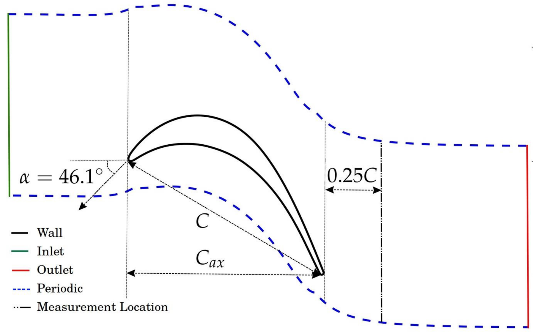
4. Numerical Setup and Configuration

The numerical setup and the flow configuration are briefly discussed in this section. The T106A LPT linear cascade was used to develop transition models with the ‘CFD-driven’ multi-objective framework. Steady, compressible and 2D RANS calculations with steady inflow conditions were conducted using the TRAF solver [41]. The focus of this study was the midspan section of the T106A LPT blade, which is the highest source of loss [6] in an LPT cascade. The midspan section can be approximated as a 2D (quasi-3D) case.

The flow configuration was chosen so that the inflow conditions, Reynolds number and Mach number match the experimentally-validated direct numerical simulation (DNS) data of Michelassi et al. [1]. The isentropic exit Reynolds number and Mach numbers were $R{e}_{2is}=100,000$ and $M{a}_{2is}=0.4$, respectively. The inlet free-stream turbulence intensity (Tu) was set to 4%.

Figure 2 shows the LPT domain used with the real (C) and axial chords $\left(C_{ax}\right)$ shown. At the inlet, the stagnation pressure and temperature along with the direction of the velocity vector (46.1${}^{\circ }$ anti-clockwise from the horizontal at the blade leading edge) are specified. The upper and bottom edges of the domain have pitchwise periodic boundary conditions. The grid, which has been used for previous studies [30,40], has approximately 83,000 points in the domain, with an O block around the blade and an H-block stitched on for the wake region. There are more than 30 points in the boundary layer with a $y^{+}<1$ for the first-off-the-wall points on both sides of the blade. An extensive grid convergence study for this grid was conducted by Akolekar [40]. All the viscous terms for the RANS calculations are discretized using second-order central difference schemes, whereas the inviscid fluxes use a second-order cell-centered scheme for discretization.

The axial distance between the inlet boundary and the blade LE was established to be consistent with the position of the turbulence generating grid in the test rig where the measurements used for validation in [38,39] were taken. Such a configuration ensured a good mesh quality and was not altered in the present work. The location of the outlet boundary of the computational domain was chosen to allow wake traversing for a range of axial distances where a possible downstream blade row is expected to sit. The presence of the H-type stitched block ensures mesh density of sufficient quality to prevent the wake from being smeared. The wake profile comparisons, which give indications on the predicted level of wake mixing, are thus expected to be significantly reliable.

5. Results and Discussions

Using single and multi-objective optimization, models are developed using the machine learning framework outlined in Section 3 for the T106A LPT linear cascade at $R{e}_{2is}=100,000$. This section discusses the performance of the models developed in terms of mean quantities such as the wall-shear stress, pressure coefficient and stagnation pressure loss profiles. Pareto analysis is also conducted to discuss the performance of the models developed via multi-objective optimization.

5.1. Single-Objective Optimization

Initially, a single-objective cost function was used to develop expressions for $f_{1a}$ and $f_{2a}$. The baseline RANS case, cost function used and the performance of the developed model are discussed in this section.

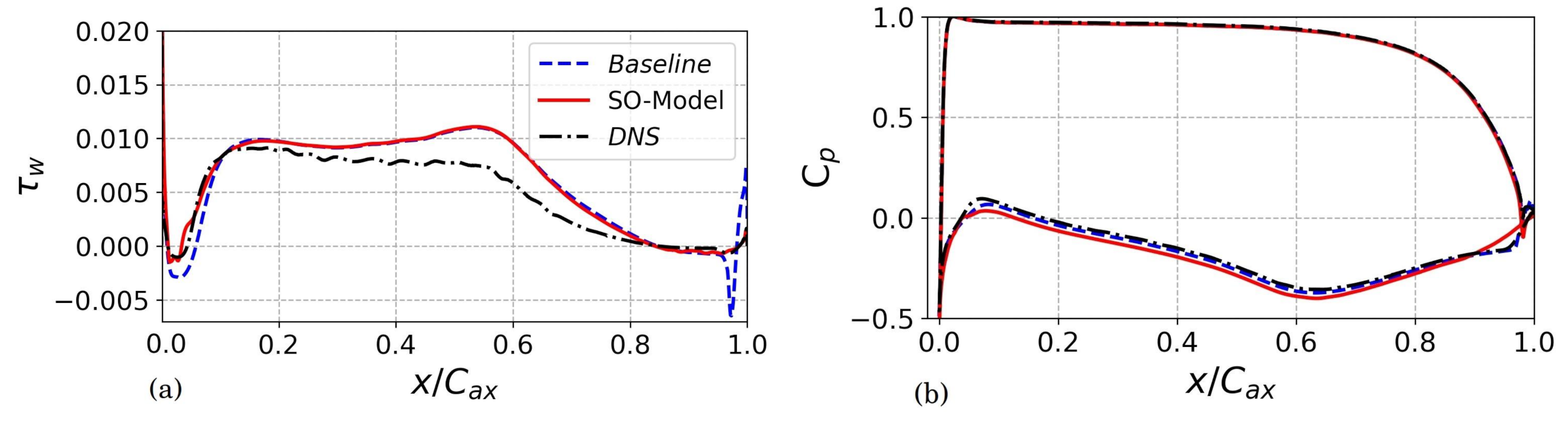
5.1.1. Baseline RANS Calculation

Figure 3 shows the suction-side wall-shear stress (${\tau }_w$) from the baseline RANS case (i.e., using the LKE model with the relations outlined in Section 2.1) and DNS data [1]. At $R{e}_{2is}=100,000$, the boundary layer separates and then reattaches, thus depicting a closed separation. In Figure 3, it is also very clear that the current baseline model does not predict the wall-shear stress accurately. What matters the most from the perspective of the boundary layer loss and subsequent downstream wake mixing loss is the accuracy of the prediction of the wall-shear stress close to and downstream of the separation onset ($x/C_{ax}\approx 0.84$).

As shown in Figure 3, the baseline LKE model offers a suitable prediction of the separation onset and extent, although the predicted reattachment occurs slightly earlier than for the high-fidelity data. The transition location, which occurs at the minimum wall-shear stress ($x/C_{ax}=0.972$), is predicted quite closely with respect to the DNS data. However, there is still plenty of scope to improve the prediction of the wall-shear stress in the separated flow regions, especially in the region leading to and immediately after the transition location (i.e., overshooting in the wall-shear stress profile).

5.1.2. Cost Function

Initially, a single-objective cost function was used in the ‘CFD-driven’ framework. This cost function revolved around minimizing the difference between the wall-shear stress obtained from RANS with respect to the one from DNS. Since the main objective of this study was to improve the separation prediction, the wall-shear stress data from $0.75\le x/C_{ax}\le 1$ was selected. The cost function ($J^{SO}$) using a single-objective function (SO-Model) is

$$J^{SO}=\sum _{x/C_{ax}=0.75}^1{\left({\tau }_w^{DNS}-{\tau }_w^{RANS}\right)}^2.$$

(11)

5.1.3. Analysis of the SO-Model

The ‘CFD-driven’ framework was able to provide suitable functional forms for $f_{1a}$ and $f_{2a}$ that significantly reduced the value of $J^{SO}$. For the baseline case, the value of the cost function is $4.147\times {10}^{-6}$, and, for the SO-model, the value of $J^{SO}$ is $0.192\times {10}^{-6}$. In order to obtain this solution, 90 generations, similar to the ‘CFD-driven’ model development for LPT wake mixing [30], were required with a population of 125 candidates. The new formulations of $f_{1a}$ and $f_{2a}$ were applied across the entire blade, even though they were developed using reference data from $0.75\le x/C_{ax}\le 1$. The wall-shear stress plot is shown in Figure 4a and the pressure coefficient plot ($C_p$) is shown in Figure 4b. The framework produces a model that results in a close match with the DNS wall-shear stress in the separated-flow region. It even gets the reattachment location predicted correctly. Since the region immediately upstream of $x/C_{ax}=0.75$ was not included in the cost function, there is not much change in the wall-shear stress behavior there. The SO-model, however, also improves the prediction of the leading-edge separation, even though that region was not included as part of the training data.

Even though the wall-shear stress prediction has improved with the SO-model, the pressure coefficient $\left(C_p\right)$ distribution has worsened over the baseline case, especially in the separated flow region on the suction-side. As the baseline case and DNS both show, there should be a plateau in the pressure coefficient plot when the flow separates. The SO-model, unlike the baseline case, does not predict a strong peak in the separated flow region in the wall-shear stress plot. The strong peak in the wall-shear stress is a peculiarity of the LKE framework, as it is the result of the turbulence ‘ignition’ by the transfer term. In the authors’ experience, the position of the minimum wall-shear stress and the subsequent ramp in wall-shear stress is crucial to get the correct pressure coefficient distribution in the separated region. As the SO-model does not show this behavior, it tends to worsen the pressure coefficient predictions over the baseline case.

5.2. Multi-Objective Optimization

Next, the multi-objective optimization approach is used to develop transition models. This section discusses the cost functions and the performance of the solutions obtained with respect to the cost functions and physical characteristics.

5.2.1. Cost Functions

The main motivation to explore the avenue of multiple cost functions was due to the worsening in the pressure coefficient prediction in the separation region on the suction-side over the baseline case when a single objective function was used. In order to at least maintain the pressure coefficient distribution as obtained from the baseline case, an additional cost function was created based on the pressure coefficient from close to peak suction right to the blade trailing edge (TE)($0.6\le x/C_{ax}\le 1$—this region includes the separation plateau). The two cost functions used are

$$\begin{array}{cc}\hfill J^{MO1}=& \sum _{x/C_{ax}=0.6}^1{\left({\tau }_w^{DNS}-{\tau }_w^{RaNS}\right)}^2,\hfill \\ \hfill J^{MO2}=& \sum _{x/C_{ax}=0.6}^1{\left(C_p^{DNS}-C_p^{RaNS}\right)}^2.\hfill \end{array}$$

(12)

The multi-objective optimization was run for 90 generations with a population of 125 individuals. In order to obtain the final solution (at n = 90), the multi-objective approach used about 1500 core hours, which was about three times that of the single-objective approach. This is because the multi-objective approach evaluates many more possible candidate solutions as opposed to a single best solution in the single-objective approach. If the data from baseline RANS calculations are fed into the cost functions, then $J^{MO1}=5.24\times {10}^{-6}$ and $J^{MO2}=3.816\times {10}^{-4}$.

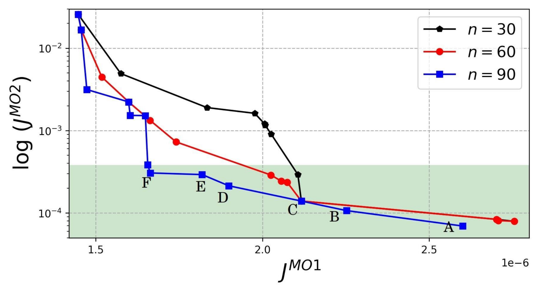
5.2.2. Pareto Analysis

The best way to analyze the evolution of the models generated with the multi-objective optimization approach is with Pareto analysis. In order to compare two candidate solutions, this optimization approach uses the concept of Pareto domination. One candidate is said to dominate the other candidate when its cost function values are all lower or equal (≤) to the dominated candidate’s values with one value being strictly lower (<). When Pareto domination is applied to the entire population via pairwise comparison, each candidate solution is assigned a rank r. Within one rank, no solution dominates another solution.

However, all solutions of rank r = k${}_1$ dominate all solutions of rank r = k${}_2$, where k${}_1$ and k${}_2$ are integer values and $k_1<k_2$. The solutions of rank r = 1 are not dominated by any other solution in the population and define what is commonly referred to as the Pareto front. Figure 5 shows the Pareto front evolution up to 90 generations (n). The value of $J^{MO1}$ and the natural logarithm of $J^{MO2}$ are shown on the x and y axes, respectively. As the generations go on increasing, the number of candidate solutions on the Pareto front go on increasing, which indicates that a better set of solutions (in terms of the cost functions) are being found with each generation. The Pareto front shifts closer to the x and y axes, indicating that the objective functions are being minimized with each progressive generation. At $N=90$, all the solutions on the Pareto fronts have a value of $J^{MO1}$, which is more than two times smaller than the baseline case. However, not all solutions offer reductions in the value of $J^{MO2}$ over the baseline case. The shaded green area in Figure 5 denotes the region in which the value of $J^{MO2}$ is less than the baseline value of $J^{MO2}=3.816\times {10}^{-4}$.

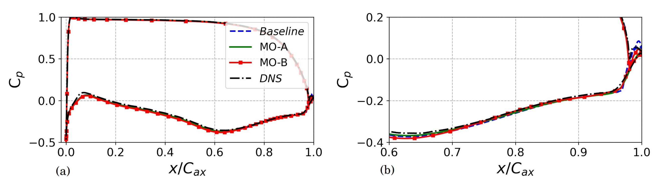
5.2.3. Analysis of Solutions

At the last generation (n = 90), every model on the Pareto front was analyzed for its performance in terms of the wall-shear stress and the pressure coefficient. It was found that only those models which reduced the value of $J^{MO2}$ over the baseline case were able to produce numerically stable solutions. Of these, solutions A and B best represented the flow physics on the blade and in the wake. Although solutions C–F reduced the value of $J^{MO2}$ over the baseline case and had lower values of $J^{MO1}$ than solutions A and B, they either predicted an early transition onset location or were unable to provide a strong peak in the separated region in the wall-shear stress profile (i.e., similar to the SO-model in Figure 4a). Absence of a strong peak in the separated flow region of the wall-shear stress profile or predicting an early onset of transition as compared to the DNS data (even with a strong peak in the separated region) resulted in excessive turbulent diffusion and some numerical instabilities in the wake. The model formulation of solution A is

$$\begin{array}{cc}\hfill & f_{1a}={\Pi }_3({\Pi }_2+{\Pi }_4-{\Pi }_3-{\Pi }_7+2)+{\Pi }_2-0.21,\hfill \\ \hfill & \psi =max(1.16-0.43{\Pi }_1+0.21{\Pi }_5-{\Pi }_6,0).\hfill \end{array}$$

(13)

The formulation of the $f_{1a}$ function highlights the leading role of the ${\Pi }_2$ term which is a vorticity scale closely related to the shear-layer vorticity thickness. This is consistent with the original modeling assumption. ${\Pi }_2$ and ${\Pi }_4$ introduce the effect of the freestream turbulence level in LKE production. The ${\Pi }_7$ term is large in the wall proximity and rapidly decays with the distance from the wall. It appears with a negative sign, and thus it tends to suppress LKE production near the wall. This is consistent with the fact that in separated laminar flows the amplification of pre-transitional fluctuations occurs in the separated shear-layer and thus far from the wall. The original formulation of the $\psi$ function employs the wall distance turbulent Reynolds number (i.e., ${\Pi }_4$) to control the transition onset. In Equation (13), it is replaced by ${\Pi }_5$. Some recently developed transition prediction frameworks [8,10] share this particular feature with the proposed one. The transition onset parameter, which is originally a constant (i.e., $C_4$), is replaced in Equation (13) by a function of ${\Pi }_1$ and ${\Pi }_6$. The effect is to delay transition as the shear-layer thickness increases (e.g., long bubbles). Additionally, the limiter $min(f_1,f_{1a})$ was also used as part of the multi-objective calculations. The use of this limiter improved the stability of the solution in the wake region. Due to the use of this limiter, the leading-edge separation prediction did not change with respect to the baseline case.

Figure 6 and Figure 7 show the pressure coefficient and suction-side wall-shear stress, respectively, for the baseline case, DNS data and the solutions A (MO-A) and B (MO-B). Both solutions not only predict the separation plateau feature in the pressure coefficient plot, as opposed to the SO-model, but they also offer an improved prediction in the separation plateau over the baseline case. This is because both the MO-A and MO-B models predict a peak (of smaller magnitude than the baseline case) in the separated flow region of the wall-shear stress profile, a necessary characteristic of the LKE modeling framework to predict a separation plateau in the pressure coefficient. These models also offer significantly better predictions of the wall-shear stress over the baseline case. They reduce the magnitude of both peaks (one at transition onset and the other one after turbulent reattachment) in the wall-shear stress by more than two times over the baseline case. The MO-A and MO-B models predict reattachment at $x/C_{ax}$ = 0.987 and $x/C_{ax}$ = 0.988, respectively, which is quite close to the DNS value of $x/C_{ax}$ = 0.986. This is an improvement over the baseline case which predicts reattachment at $x/C_{ax}$ = 0.982. Consequently, these models have a positive impact on the wake mixing prediction.

Figure 8 shows the stagnation pressure loss at 25%C downstream of the blade TE (see Figure 2). The stagnation pressure loss (${\Omega }^{*}$) is defined as

$${\Omega }^{*}\left(y^{*}\right)=\frac{P_{t,1}-P_t\left(y^{*}\right)}{P_{t,1}-P_2},$$

(14)

where $P_{t,1}$ is the inlet stagnation pressure, $P_2$ is the exit static pressure, $P_t\left(y^{*}\right)$ is the stagnation pressure at the location of interest and $y^{*}$ is a pitchwise normalized coordinate defined as $y^{*}=(y-y_{max})/(y_{max}-y_{min})$.

Since the MO-A and MO-B models are able to predict the flow coming off the blade TE quite accurately with respect to the high-fidelity data, the resulting stagnation pressure loss profiles (and thus the wake mixing) are also better predicted than the baseline case. These models improve the prediction of the peak wake loss error and increase the width of the profile, indicating additional diffusion in the wake over the baseline case. It is to be noted that the Boussinesq approximation was used in the wake region for the baseline and MO models. The wake mixing prediction can be further improved by using machine-learned EARSMs. However, further enhancing the wake mixing prediction was not addressed in this work, as this is considered separately in [25,29,30]. The ‘CFD-driven’ canonical-wake EARSM of Akolekar et al. [30] is apt for further improving the wake mixing prediction for this particular case. The canonical-wake model has been formulated such that it can improve the wake evolution when the flow coming off the blade TE is accurately predicted.

In summary, including an additional cost function based on the suction-side pressure coefficient was an immense benefit to formulate models which preserve the integrity of the LKE modeling framework and improve the prediction of the physical characteristics of the flow, not only in the separation region but also downstream of the blade TE.

6. Conclusions

This study used a multi-objective ‘CFD-driven’ algorithm to enhance the prediction of separated flow transition of the T106A LPT blade at $R{e}_{2is}=100,000$. The existing LKE transition model struggles to accurately predict the wall-shear stress in the separated flow region, and thus the wake mixing downstream of the blade TE is also poorly predicted. Using the ‘CFD-driven’ multi-objective framework and seven non-dimensional pi groups, model formulations for the transition parameter $\psi$ and the $f_{1a}$ term in the laminar eddy viscosity are proposed. Initially, a single-objective approach was explored, using the wall-shear stress from DNS data in the separation region as a reference. The resulting SO-model was able to predict the wall-shear stress surprisingly close to the DNS. However, as there was no strong peak in the separation region of the wall-shear stress profile (which is a result of turbulence ignition by the transfer term), the prediction of the separation plateau in the pressure coefficient plot worsened over the baseline case.

In order to account for this deficiency of the SO-model, multi-objective optimization was used and an additional cost function which included the suction-side pressure coefficient was introduced. Pareto analysis was used to assess the performance of the models developed. It was found that only those models which reduced the value of the pressure coefficient cost function over the baseline case produced numerically stable solutions. Two of these models were able to preserve the integrity of the LKE framework (i.e., strong peak in the separated region) as well as improved the prediction of physical characteristics of the transition process such as the reattachment location and magnitudes of the peaks in the wall-shear stress profile. Thus, the overall structure of the separation bubble was improved. Since these models were able to closely match the flow coming off the blade TE, the resulting turbulent diffusion in the wake was increased. This resulted in better prediction of wake loss profiles with respect to high-fidelity data.

Overall, a promising framework for multi-objective and multi-expression ‘CFD-driven’ model development using non-dimensional pi groups was explored. To the authors’ knowledge, this is the first known study which makes use of data-driven machine learning tools to enhance the prediction of separation-induced transition in LPTs. Additional analyses and development is required to test this framework and resulting models across different operating conditions and geometries.

References

1. Michelassi, V.; Chen, L.W.; Pichler, R.; Sandberg, R.D. Compressible Direct Numerical Simulation of Low Pressure Turbine—Part II: Effect of Inflow Disturbances. J. Turbomach. 2015, 137, 71005. [Google Scholar] [CrossRef]
2. Hodson, H.P.; Howell, R.J. Bladerow Interactions, Transition, and High-Lift Aerofoils in Low-Pressure Turbines. Annu. Rev. Fluid Mech. 2005, 37, 71–98. [Google Scholar] [CrossRef]
3. Mayle, R.E. The Role of Laminar-Turbulent Transition in Gas Turbine Engines. J. Turbomach. 1991, 113, 509–537. [Google Scholar] [CrossRef]
4. Schlichting, H.; Gersten, K. Boundary Layer Theory; Springer: Berlin/Heidelberg, Germany, 1999. [Google Scholar]
5. Stieger, R.D.; Hodson, H.P. The Transition Mechanism of Highly-Loaded LP Turbine Blades. J. Turbomach. 2004, 126, 536–543. [Google Scholar] [CrossRef]
6. Denton, J.D. The 1993 IGTI Scholar Lecture: Loss Mechanisms in Turbomachines. J. Turbomach. 1993, 115, 621. [Google Scholar] [CrossRef]
7. Michelassi, V.; Chen, L.; Pichler, R.; Sandberg, R.; Bhaskaran, R. High-Fidelity Simulations of Low-Pressure Turbines: Effect of Flow Coefficient and Reduced Frequency on Losses. J. Turbomach. 2016, 138, 111006. [Google Scholar] [CrossRef]
8. Dick, E.; Kubacki, S. Transition Models for Turbomachinery Boundary Layer Flows: A Review. Int. J. Turbomach. Propuls. Power 2017, 2, 4. [Google Scholar] [CrossRef] [Green Version]
9. Menter, F.R.; Langtry, R.B.; Likki, S.R.; Suzen, Y.B.; Huang, P.G. A Correlation-Based Transition Model Using Local Variables—Part I: Model Formulation. J. Turbomach. 2006, 128, 413–422. [Google Scholar] [CrossRef]
10. Walters, D.K.; Cokljat, D. A Three-Equation Eddy-Viscosity Model for Reynolds-Averaged Navier-Stokes Simulations of Transitional Flow. J. Fluids Eng. 2008, 130, 121401. [Google Scholar] [CrossRef]
11. Pacciani, R.; Marconcini, M. Calculation of High-Lift Cascades in Low Pressure Turbine Conditions Using a Three-Equation Model. J. Turbomach. 2011, 133, 1–9. [Google Scholar] [CrossRef]
12. Brunton, S.L.; Noack, B.R.; Koumoutsakos, P. Machine Learning for Fluid Mechanics. Annu. Rev. Fluid Mech. 2020, 52, 477–508. [Google Scholar] [CrossRef] [Green Version]
13. Duraisamy, K.; Spalart, P.R.; Rumsey, C.L. Status, Emerging Ideas and Future Directions of Turbulence Modeling Research in Aeronautics; Technical Report November; NASA: Hampton, VA, USA, 2017.
14. Medic, G. Impact of Vision 2030 on CFD Practices in Propulsion Industry. In Proceedings of the AIAA Aviation 2019 Forum, Dallas, TX, USA, 17–21 June 2019. [Google Scholar]
15. Runchal, A.K.; Rao, M.M. CFD of the Future: Year 2025 and Beyond. In 50 Years of CFD in Engineering Sciences; Springer: Berlin/Heidelberg, Germany, 2020. [Google Scholar]
16. Ling, J.; Jones, R.; Templeton, J. Machine learning strategies for systems with invariance properties. J. Comput. Phys. 2016, 318, 22–35. [Google Scholar] [CrossRef] [Green Version]
17. Milani, P.M.; Ling, J.; Eaton, J.K. Turbulent Scalar Flux in Inclined Jets in Crossflow: Counter Gradient Transport and Deep Learning Modelling. J. Fluid Mech. 2021, 906. [Google Scholar] [CrossRef]
18. Milani, P.M.; Ling, J.; Saez-Mischlich, G.; Bodart, J.; Eaton, J.K. A Machine Learning Approach for Determining the Turbulent Diffusivity in Film Cooling Flows. J. Turbomach. 2018, 140, 021006. [Google Scholar] [CrossRef] [Green Version]
19. Milani, P.M.; Ling, J.; Eaton, J.K. Physical Interpretation of Machine Learning Models Applied to Film Cooling Flows. J. Turbomach. 2019, 141, 011004. [Google Scholar] [CrossRef]
20. Duraisamy, K.; Iaccarino, G.; Xiao, H. Turbulence Modeling in the Age of Data. Annu. Rev. Fluid Mech. 2019, 53, 357–377. [Google Scholar] [CrossRef] [Green Version]
21. Duraisamy, K. Machine Learning Augmented Reynolds-Averaged & Large eddy Simulation Models of Turbulence. arXiv 2021, arXiv:2009.10675v3. [Google Scholar]
22. Ferreira, C. Gene Expression Programming: A New Adaptive Algorithm for Solving Problems. Complex Syst. 2001, 13, 87–129. [Google Scholar]
23. Weatheritt, J.; Sandberg, R.D. A Novel Evolutionary Algorithm Applied to Algebraic Modifications of the RANS Stress-Strain Relationship. J. Comput. Phys. 2016, 325, 22–37. [Google Scholar] [CrossRef]
24. Akolekar, H.D.; Sandberg, R.D.; Hutchins, N.; Michelassi, V.; Laskowski, G. Machine-Learnt Turbulence Closures for Low Pressure Turbines with Unsteady Inflow Conditions. J. Turbomach. 2019, 141, 101009. [Google Scholar] [CrossRef]
25. Akolekar, H.D.; Weatheritt, J.; Hutchins, N.; Sandberg, R.D.; Laskowski, G.; Michelassi, V. Development and Use of Machine-Learnt Algebraic Reynolds Stress Models for Enhanced Prediction of Wake Mixing in Low-Pressure Turbines. J. Turbomach. 2019, 141, 041010. [Google Scholar] [CrossRef]
26. Parneix, S.; Laurence, D.; Durbin, P.A. A Procedure for Using DNS Databases. J. Fluids Eng. 1998, 120, 40–46. [Google Scholar] [CrossRef]
27. Akolekar, H.D.; Zhao, Y.; Sandberg, R.D.; Hutchins, N.; Michelassi, V. Turbulence Model Development for Low & High Pressure Turbines Using a Machine Learning Approach. In Proceedings of the 24th International Society of Air Breathing Engines, Canberra, Australia, 22–27 September 2019. [Google Scholar]
28. Weatheritt, J.; Pichler, R.; Sandberg, R.D.; Laskowski, G.; Michelassi, V. Machine Learning for Turbulence Model Development Using a High Fidelity HPT Cascade Simulation. In Proceedings of the Turbo Expo: Power for Land, Sea, and Air, Charlotte, NC, USA, 26–30 June 2017. [Google Scholar]
29. Zhao, Y.; Akolekar, H.D.; Weatheritt, J.; Michelassi, V.; Sandberg, R.D. RANS Turbulence Model Development Using CFD-Driven Machine Learning. J. Comput. Phys. 2020, 411, 109413. [Google Scholar] [CrossRef] [Green Version]
30. Akolekar, H.D.; Zhao, Y.; Sandberg, R.D.; Pacciani, R. Integration of Machine Learning and Computational Fluid Dynamics to Develop Turbulence Models for Improved Low Pressure Turbine Wake Mixing Predictions. J. Turbomach. 2021, 143, 121001. [Google Scholar] [CrossRef]
31. Waschkowski, F.; Zhao, Y.; Sandberg, R.; Klewicki, J. Multi-Objective CFD-Driven Development of Coupled Turbulence Closure Models. arXiv 2021, arXiv:2105.06225. [Google Scholar]
32. Zafar, M.I.; Xiao, H.; Choudhari, M.M.; Li, F.; Chang, C.L.; Paredes, P.; Venkatachari, B. Convolutional Neural Network for Transition Modeling Based on Linear Stability Theory. Phys. Rev. Fluids 2020, 5, 1–15. [Google Scholar] [CrossRef]
33. Yang, M.; Xiao, Z. Improving the k-ω-γ-Ar Transition Model by the Field Inversion and Machine Learning Framework. Phys. Fluids 2020, 32, 064101. [Google Scholar]
34. White, F.M. Fluid Mechanics; McGraw Hill: New York, NY, USA, 2017. [Google Scholar]
35. Mayle, R.; Schulz, A. The Path to Predicting Bypass Transition. J. Turbomach. 1997, 119, 405–411. [Google Scholar] [CrossRef]
36. Lardeau, S.; Leschziner, M.A.; Li, N. Modelling Bypass Transition with Low-Reynolds-Number Nonlinear Eddy-Viscosity Closure. Flow Turbul. Combust. 2004, 73, 49–76. [Google Scholar] [CrossRef]
37. Schmitt, G. About Boussinesq’s Turbulent Viscosity Hypothesis: Historical Remarks and a Direct Evaluation of its Validity. Comptes Rendus Mec. Elsevier Masson 2007, 335, 617–627. [Google Scholar] [CrossRef] [Green Version]
38. Pacciani, R.; Marconcini, M.; Arnone, A.; Bertini, F. An Assessment of the Laminar Kinetic Energy Concept for the Prediction of High-Lift, Low-Reynolds Number Cascade Flows. Proc. Inst. Mech. Eng. Part A J. Power Energy 2011, 225, 995–1003. [Google Scholar] [CrossRef]
39. Pacciani, R.; Marconcini, M.; Arnone, A.; Bertini, F. Predicting High-Lift Low-Pressure Turbine Cascades Flow Using Transition-Sensitive Turbulence Closures. J. Turbomach. 2014, 136, 051007. [Google Scholar] [CrossRef]
40. Akolekar, H.D. Turbulence Model Development and Implementation For Low Pressure Turbines Using a Machine Learning Approach. Ph.D. Thesis, University of Melbourne, Melbourne, Australia, 2019. [Google Scholar]
41. Arnone, A.; Liou, M.S.; Povinelli, L.A. Navier-Stokes Solution of Transonic Cascade Flows Using Non-Periodic C-Type Grids. J. Propuls. Power 1992, 8, 410–417. [Google Scholar] [CrossRef]
Figure 1. ‘CFD-driven’ transition model development with the multi-objective and multi-expression approach.
Energies 14 04680 g001
Figure 2. The T106A blade geometry and computational domain with boundary conditions.
Energies 14 04680 g002
Figure 3. (a) Suction-side wall-shear stress from the baseline LKE model and DNS. (b) Zoomed view of the wall-shear stress in the separated flow region, near the blade trailing edge.
Energies 14 04680 g003
Figure 4. (a) Suction-side wall-shear stress and (b) pressure and suction-side pressure coefficient for the SO-Model, baseline case and DNS.
Energies 14 04680 g004
Figure 5. Evolution of the Pareto front across 90 generations.
Energies 14 04680 g005
Figure 6. (a) Pressure coefficient with the various multi-objective optimized models. (b) Zoomed view of the suction-side pressure coefficient in the separated flow region, near the blade trailing edge.
Energies 14 04680 g006
Figure 7. (a) Suction-side wall-shear stress with the various multi-objective optimized models. (b) Zoomed view of the suction-side wall-shear stress in the separated flow region, near the blade TE.
Energies 14 04680 g007
Figure 8. Stagnation pressure loss profiles 25%C downstream of the blade TE.
Energies 14 04680 g008
Publisher’s Note: MDPI stays neutral with regard to jurisdictional claims in published maps and institutional affiliations.