Impact of Cryogenics on Cavitation through an Orifice: A Review

Abstract

Cryogenic cavitation affects the operation of liquid propulsion systems during the first phase of a launch. Its effects within orifices or turbopumps can range from mild instabilities to catastrophic damages to the structures, jeopardizing the launch itself. Therefore, to ensure the proper designing of propulsion systems, cavitation phenomena cannot be neglected. Although hydrodynamic cavitation has been studied for decades, the impact of the nature of the fluid has been sparsely investigated. Therefore, this review, beginning from the basic concepts of cavitation, analyzes the literature dedicated to hydrodynamic cryogenic cavitation through an orifice. Our review provides a clear vision of the state-of-the-art from experimental and modeling viewpoints, identifies the knowledge gaps in the literature, and proposes a way to further investigate cryogenic cavitation in aerospace science.

1. Introduction

Propulsion systems in liquid rocket engines are strongly affected by multi-phase transient and thermal phenomena during their startup phases. When a spacecraft is launched, the propellant tanks are pressurized, and the latch valve opens to fill and pressurize the propellant lines of the spacecraft. This is the moment when a two-phase flow is produced, first due to the chilldown of the propellant line, then to cavitation, impending from the passage of the fluid through valves or other restrictions, and from fluid hammer transients caused by the rapid opening of the valve. Among the phenomena mentioned above, cavitation plays a critical role in designing the propellant line system, including valves and other singularities. Although hydrodynamic cavitation has been investigated for decades, its prediction when using cryogenic fluids is still hard to achieve. The limiting factor is the difficulty in describing highly non-equilibrium thermodynamic processes in terms of simplified and computationally efficient models based on equilibrium thermodynamic assumptions. In this review, we start with the basic concept of hydrodynamic cavitation through an orifice. We critically analyze, from experimental and modeling viewpoints, the impact of the cryogenic nature of the fluid. We identify and evaluate the principal knowledge gaps and the open research questions regarding the thermodynamic effects on hydrodynamic cavitation.

1.1. Statement of the Problem

The simplest geometry to study cavitation is an orifice, schematized in Figure 1. The liquid upstream and downstream pressures are $P_{up}$ and $P_{dw}$, respectively, and D is the pipe diameter, while s and d are, respectively, the thickness and the diameter of the orifice. The pressure drop $\Delta P=P_{up}-P_{dw}$ determines the flow rate Q. $\Delta P$ may reach large enough values that bring the fluid at the vena contracta, at a pressure below the local fluid saturation $P_{sat}\left(T\right)$ producing cavitation. As a consequence, a pressure pulsation with amplitude $P_A$ and frequency f is observed.

Assuming a fixed orifice geometry and constant fluid properties, the cavitation problem relies on the maximum pressure drop $P_{up}-P_{min}$ and $P_{dw}$. The cavitation condition strength, $\sigma$, reads as:

$$\sigma =\frac{P_{up}-P_{min}}{P_{up}-P_{dw}}$$

(1)

The minimal pressure $P_{min}$ is assumed to be, in isothermal cavitation, the saturation pressure of the liquid at the local temperature $P_{sat}$ [1,2,3]. Very often, experimental works provide $\sigma$ as the only parameter to define the cavitation conditions [4,5]. As highlighted by [6], all of these efforts to give precise values of $\sigma$ become useless and cause inconsistencies if very little information is provided about other flow parameters, e.g., flow velocity, downstream pressure, and pressure fluctuations. In this context, Reference [7] proposed to use $\xi$ as a second parameter, accounting for the downstream pressure. Namely, $\xi$ is the ratio between the pressure at which the vapor bubble is produced, approximately $p\sim P_{sat}$, and the pressure that it experiences traveling downstream, i.e., $p\sim P_{dw}$.

$$\xi =\frac{P_{sat}}{P_{dw}}$$

(2)

Concerning the flow velocity and the pressure fluctuations, the three dimensionless quantities completing the characterization of the cavitating regimes are:

$$\begin{array}{cc}\hfill \widehat{Q}& =\frac{Q}{\pi \frac{d^2}{4}\sqrt{\Delta P/\rho }}\hfill \end{array}$$

(3a)

$$\begin{array}{cc}\hfill St& =\frac{fd}{\sqrt{\Delta P/\rho }}\hfill \end{array}$$

(3b)

$$\begin{array}{cc}\hfill {\widehat{P}}_A& =\frac{P_A}{P_{up}-P_{sat}}\hfill \end{array}$$

(3c)

where the second dimensionless group, Equation (3b), is the well known Strouhal number.

In case of cryogenic fluid, the approximation $P_{min}\sim P_{sat}$ can fail, since the thermodynamic state strongly influences both the cavitation occurrence and its regime [8] and the fluid temperature varies during the phase change. Therefore, to correctly describe the phenomenon, two more parameters must be considered, i.e., the subcooling degree $\Delta T_{sub}$ and the superheat $R_p$:

$$\Delta T_{sub}=\frac{T_{sat}\left(P_{up}\right)-T_{up}}{T_{cri}}{R}_p=\frac{P_{sat}\left(T_{up}\right)}{P_{dw}}.$$

(4)

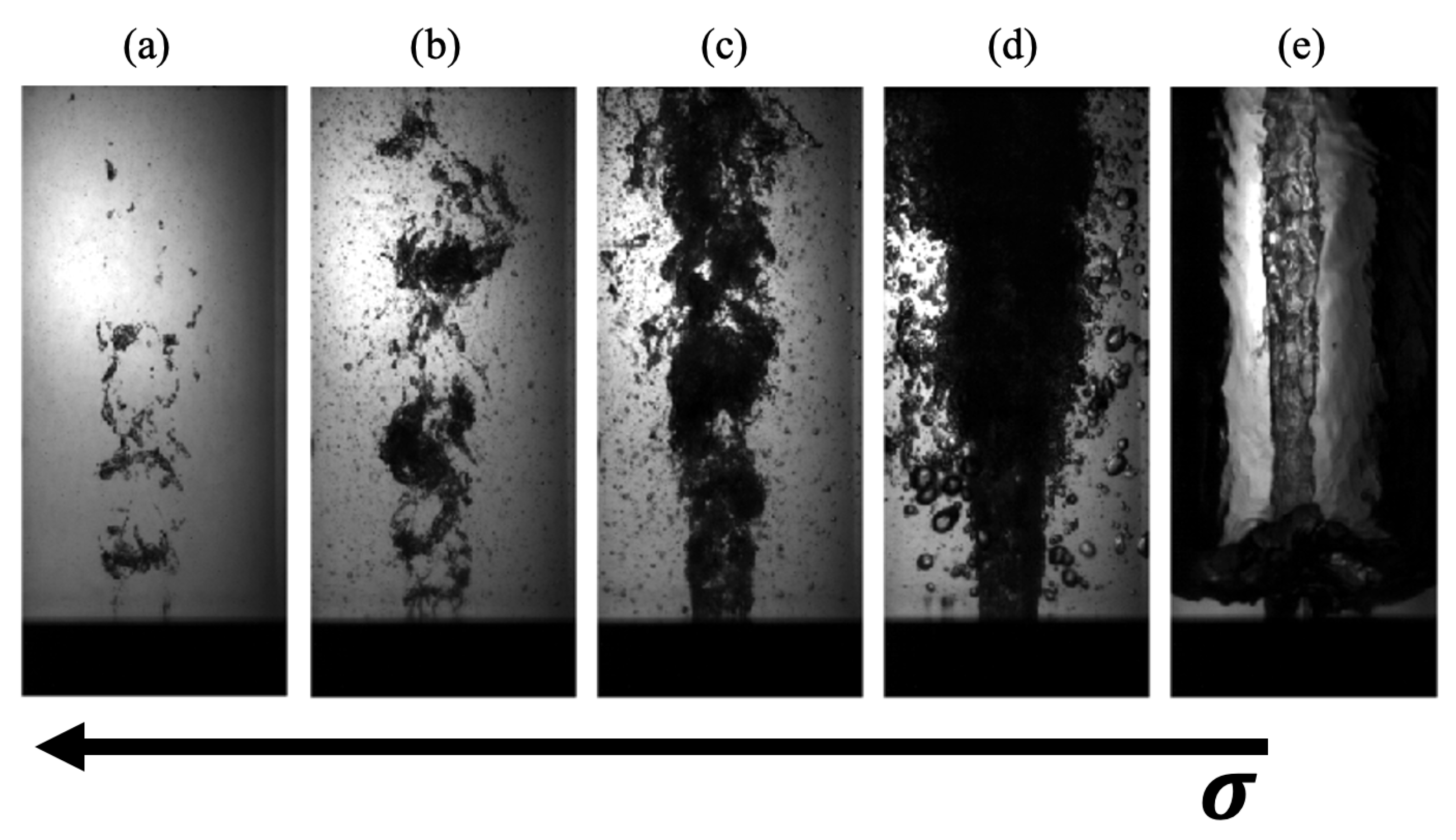
1.2. Cavitation Regimes

The cavitation inception [1,9] takes place as the intermittent appearance of the first tiny bubbles, but the pressure downstream of the orifice is still higher than the saturation one. This triggering of cavitation is considered to be strongly affected by the gaseous cavitation, which is the diffusion of dissolved gases into the available nuclei in the liquid [1,10]. Indeed, dissolved gases make the bubble growth easier by lowering the pressure threshold to be overcome [11,12]. As the process develops, bubbles grow and form clouds that periodically shed and collapse in the channel at higher pressures (Figure 2b,c). Within this regime, the size of the vapor clusters increases progressively and the flow chokes through the orifice [7]. In the literature, the non-recoverable stage of cavitation is referred to as super-cavitation [1] (Figure 2e) or flashing [13]. Vapor bubbles do not collapse anymore, and the average pressure at around six pipe diameters far from the orifice [14] is still the vapor pressure. It is worth noting that the terms super-cavitation and flashing identify a similar phenomenon. However, flashing is generally used when the transition from the vapor back to liquid is caused by a temperature decrease rather than from the pressure recovery [14]. Therefore, the term flashing is found when dealing with cavitation in fluids with strong thermodynamic effects, whereas super-cavitation is the term preferred for isothermal cavitation, e.g., cavitation in water [1,15].

1.3. Thermodynamic Effect

The thermodynamic effect is a localized cooling process that takes place during the cavitation mechanism [16] since the liquid surrounding the vapor bubble releases latent heat. This effect is usually neglected and cavitation is considered an isothermal process. However, in the case of cryogenic fluids, such an approximation is no longer correct. To understand why this effect must be taken into account, Franc [17] suggests looking at the heat balance

$${\rho }_v{V}_v{L}_{vap}={\rho }_l{V}_l{C}_{pl}\Delta T$$

(5)

where $L_{vap}$ is the latent heat of vaporization, and $C_{pl}$ is the specific heat. The liquid and vapor phase are referred by the subscripts l and v, respectively. Some terms of Equation (5) are commonly grouped [18] to define the characteristic temperature difference

$$\Delta T^{*}=\frac{{\rho }_v{L}_{vap}}{{\rho }_l{C}_{pl}}$$

(6)

It stands for the temperature drop needed to transform a fixed liquid volume ($V_l$) into vapor. This temperature drop ($\Delta T^{*}$) depends only on the physical properties of the liquid.

Table 1. Characteristic values for water compared to cryogenic liquids. The values are extracted from the NIST database [19].

	H${}_2$O	LO${}_{\mathit{x}}$	LN${}_2$	LCH${}_4$	LH${}_2$
T$\left[K\right]$	$303.16$	$108.81$	$93.99$	$135.35$	$27.24$
$C_{pl}$$[J/g·K]$	$4.18$	$1.80$	$2.20$	$3.73$	$16.41$
${\rho }_v/{\rho }_l$	$3.05\times {10}^{-5}$	$0.02$	$0.03$	$0.02$	$0.10$
$L_{vap}$$[J/g]$	$2429.82$	$191.38$	$173.32$	$458.25$	$372.76$
$\Delta T^{*}$	$0.02$	$0.95$	$1.12$	$2.55$	$2.81$

shows these characteristic properties at a pressure of 500 kPa for water and four cryogenic liquids, namely, oxygen, nitrogen, methane, and hydrogen. By looking at the $\Delta T^{*}$ values, one may see the distinction between isothermal liquids as water and thermosensitive liquids as the cryogenic ones, whose $\Delta T^{*}$ is much bigger than for the water and, consequently, temperature depression during cavitation is much more significant.

Tani and Nagashima [20] observed this thermodynamic effect compared cavitation through a nozzle with both water and liquid nitrogen. Figure 3 shows the correspondence between the vapor fraction increase after the throat (b) and the temperature reduction (a) when testing LN${}_2$. On the contrary, no change of temperature (c) appeared for water when the flow quality increases (d).

The impact of the evaporative cooling on the vapor bubbles shape is addressed both by Hosangadi and Ahuja [21] and by Tseng and Shyy [22]. Since the temperature drops inside a bubble, the local vapor pressure reduces as well. This means a higher local cavitation number $\left(\sigma \right)$, resulting in smaller bubbles, which, in turn, spread out more laterally. Figure 4 shows the void fraction for both isothermal and cryogenic cavitation.

Tseng and Shyy [22] proposed a turbulence model that enables reducing the uncertainty on the turbulent parameters. The influence of turbulence on the thermodynamic effect is also investigated by Niiyama et al. [23]. They observed that the turbulent intensity decreases with the cavitation number due to the increase in the void fraction. On the other hand, by keeping $\sigma$ constant, a higher Reynolds number enhances the thermal transport and leads to a more intense turbulent heat transfer. Interestingly, the authors also observed that turbulence contrasts the delay in the bubble growth due to the thermal effects, inducing a temperature rise in the area populated by the bubbles.

2. Cavitation Modeling

Cavitation modeling presents non-negligible difficulties that arise from the complex nature of this kind of two-phase flow. During cavitation, a thermodynamic phase transition occurs and the flow undergoes important changes in local density and speed of sound. Moreover, the large variance in the nuclei number and size and the interaction with turbulence make cavitation a stochastic process. Realistic models should take into account the whole phenomenon: from the cavitation inception, when vapor bubbles start forming, up to the super-cavitation. Up until now, different models have been proposed in the literature [24]. In the following, they will be examined and classified into three different categories: (1) the bubbly flow models; (2) the homogeneous mixture models; and (3) the multiphase models.

2.1. Bubbly Flow Models

The liquid phase is modeled with the continuity, momentum, and energy equation. This set of equations is coupled with the Rayleigh–Plesset equation, which models the bubble dynamics. Franc et al. [25] implemented this model with sheet cavitation in an inducer, and included the thermal effects. The resulting Rayleigh equation reads as

$$R\frac{d^{2}R}{d{t}^2}+\frac{3}{2}{\left(\frac{dR}{dt}\right)}^2=\frac{p_v\left(T_c\right)-p\left(T_{\infty }\right)}{{\rho }_l}-U_u^2\frac{C_p+{\sigma }_v}{2}$$

(7)

where R is the bubble radius, $p_v$ the vapor pressure at the actual bubble temperature $T_c$, ${\rho }_l$ the liquid density, $T_{\infty }$ the liquid temperature at infinity, $U_u$ the upstream relative flow velocity, and $C_p$ the pressure coefficient. In the definition of the cavitation number ${\sigma }_v$, the vapor pressure is calculated at $T_{\infty }$, and the relation is

$${\sigma }_v=\frac{p_u-p_v\left(T_{\infty }\right)}{0.5{\rho }_l{U}_u^2}$$

(8)

Two approaches are considered to determine the bubble temperature: the convective approach and the conductive one. The difference is the parameter controlling the thermal effects. In the first one, this role is given to the heat transfer coefficient, whereas, in the second one, it is left to $\mathcal{E}$, the ratio between the eddy thermal diffusivity and the liquid molecular thermal one. These approaches showed different results in terms of temperature distribution and cavity length; however, they seemed to converge to the same solution when thermal effects were predominant.

2.2. Homogeneous Models

The homogeneous models consider the two phases as a continuum and Euler equations are solved for the mixture. Within this category, models can be further distinguished according to the way the thermodynamic behavior of the mixture is treated. In the homogeneous equilibrium approach, kinematic and thermodynamic equilibrium are stated on the assumption that bubbles are dispersed in the liquid. To close the system of equations, two formulations are usually suggested for cavitating flows: a mixture of stiffened gas [26] and a barotropic equation of state [26,27]. As for the first cavitation model, the stiffened gas equation of state is given by:

$$\begin{array}{cc}\hfill p(\rho ,e_{☆})& =(n-1)(e_{☆}-q)\rho -n{p}_{\infty }\hfill \end{array}$$

(9a)

$$\begin{array}{cc}\hfill e_{☆}(\rho ,T)& =T·C_v\frac{p+n{p}_{\infty }}{p+p_{\infty }}+q\hfill \end{array}$$

(9b)

$$\begin{array}{cc}\hfill h\left(T\right)& =n{c}_{v}T\hfill \end{array}$$

(9c)

The polytropic coefficient n is the ratio between the specific heat capacities $(n=c_p/c_v)$, $e_{☆}$ is the internal energy and q is the fluid energy. The expressions for temperature and pressure of the mixture are deduced by assuming mechanical and thermal equilibrium. These two quantities are functions of the void fraction $\left(\alpha \right)$, which is calculated for each phase at saturation from the internal energy equation.

On the contrary, the barotropic law for water is defined as:

$$p(\rho ,\alpha )=p_{sat}+\left(\frac{{\rho }_l^{sat}-{\rho }_v^{sat}}{2}\right)c_{min}^{2}arcsin\left(A^{*}(1-2\alpha )\right)$$

(10)

The constant $A^{*}$ was introduced in [26] to also use Equation (10) in presence of pure compressible phases, i.e., $\alpha =0$. Otherwise, the speed of sound would be infinite for this condition. The parameter $c_{min}$ stands for the minimum speed of sound of the mixture. By introducing this term, non-equilibrium effects are included in the pressure. This barotropic model seems more accurate than the mixture of the stiffened gas model. In fact, concerning the Venturi geometry used in [26], it provided results in agreement with experimental data. These results are intended in terms of both velocity profiles and void fraction. It is also true that the stiffened gas mixture has yielded to a stable cavitation sheet, which completely disagrees with the experimental work. Concerning the formulation using the barotropic equation of state, Hickel et al. [28] validated it, performing large eddy simulations in a cavitating microchannel. In this work, the LES proved to resolve the dynamics of the compressible fluid and the turbulence production in shear layers.

The second approach, also known as the drift flux model, aims to take thermodynamic non-equilibrium into account. The drawback of these models is that they require specific assumptions linked to the particular geometry and conditions. Source terms for the phase change, namely the evaporation and condensation rates, can be very different according to the specific problem to deal with. To formalize this model, the following equations are considered: the conservative form of the Favre-averaged Navier–Stokes equations, a transport equation for the phase change, the energy equation in terms of enthalpy and the turbulence model.

$$\begin{array}{cc}\hfill \frac{\partial {\rho }_m}{\partial t}& +\frac{\partial \left({\rho }_m{U}_j\right)}{\partial x_j}=0\hfill \\ \hfill \frac{\partial \left({\rho }_m{U}_j\right){\rho }_m}{\partial t}& +\frac{\partial \left({\rho }_m{U}_i{U}_j\right)}{\partial x_j}=-\frac{\partial p}{\partial x_j}+\hfill \end{array}$$

(11a)

$$\begin{array}{cc}\hfill & +\frac{\partial }{\partial x_j}\left[({\mu }_m+{\mu }_T)\left(\frac{\partial U_i}{\partial x_j}+\frac{\partial U_j}{\partial x_i}-\frac{2}{3}\frac{\partial U_k}{\partial x_k}{\delta }_{ij}\right)\right]\hfill \\ \hfill \frac{\partial }{\partial t}\left({\rho }_m\left(f_L{L}_{vap}\right)\right)& +\frac{\partial }{\partial x_j}\left({\rho }_m{U}_j(H+f_L{L}_{vap})\right)=\hfill \end{array}$$

(11b)

$$\begin{array}{cc}\hfill & =\frac{\partial }{\partial x_j}\left[\left(\frac{{\mu }_m}{P{r}_{La}}+\frac{{\mu }_T}{P{r}_T}\right)\frac{\partial H}{\partial x_j}\right]\hfill \end{array}$$

(11c)

$$\begin{array}{cc}\hfill \frac{\partial {\rho }_l(1-\alpha )}{\partial t}& +\frac{\partial \left({\rho }_l(1-\alpha )U_j\right)}{\partial x_j}={\dot{m}}^{+}+{\dot{m}}^{-}\hfill \end{array}$$

(11d)

$$\begin{array}{cc}\hfill {\rho }_m& ={\rho }_l(1-\alpha )+{\rho }_v\alpha \hfill \end{array}$$

(11e)

In Equations (11), ${\rho }_m$ is the mixture density, whose expression is written in Equation (11e), $f_L$ the mass volume fraction, H is the enthalpy, and $P{r}_L$ and $P{r}_T$ are the laminar and turbulent Prandtl number, respectively. The mixture laminar viscosity is indicated as ${\mu }_m$ and the turbulence one as ${\mu }_T$. Finally, ${\dot{m}}^{+}$ and ${\dot{m}}^{-}$ are the source and the sink terms representing the condensation and evaporation rate during the cavitation process. The equations for the mass transfer read as:

$$\begin{array}{c}\hfill {\dot{m}}^{-}=\frac{C_{dest}(1-\alpha )}{t_{\infty }}\frac{{\rho }_l}{{\rho }_v}\frac{MIN(p-p_v\left(T\right),0)}{0.5{\rho }_l{U}_{\infty }^2}forp<p_v\end{array}$$

(12a)

$$\begin{array}{c}\hfill {\dot{m}}^{+}=\frac{C_{prod}\alpha }{t_{\infty }}\frac{MAX(p-p_v\left(T\right),0)}{0.5{\rho }_l{U}_{\infty }^2}forp>p_v\end{array}$$

(12b)

where $C_{dest}$ and $C_{prod}$ are two empirical constants. Their values differ significantly from one work to another, see for example [29,30,31].

The dependence of such parameters from the experiments is common to different models and poses some issues to correctly estimating the cavity shape and the pressure distribution. The problem is that, although the evaporation and condensation coefficient are case-dependent, a common routine is to use constant values for the numerical simulations. An attempt to get rid of these empirical factors is found in Senocak et al. [32]. They propose a new interfacial dynamics cavitation model developed from the conservation of the mass and the normal-momentum at the liquid–vapor interface. Based on dimensional analysis, the two source terms are built from the definition of the liquid volume fraction at the interface. Thus, they could replace the two empirical coefficients with terms depending on the interface properties. Recently, Jin et al. [33] designed a model to relate the values of the condensation and evaporation coefficients to the operating conditions, trying, in this way, to overcome the limitation of using empirical constants. Other examples of optimization of these empirical parameters are the surrogate-based sequential approximate optimization (SAO) method considered by Zhou et al. [34] or the machine learning method employed by Sikirica et al. [35]. Both were applied within the Kunz mixture cavitation model and provided better performances in cavitation prediction and simulation than the use of constant coefficients.

The drift flux model has also been implemented in FLUENT6.1 [13] to predict a flashing flow through a nozzle. Previous models, such as [36], underestimated the pressure at the inlet of the nozzle and the void fraction in the flashing flow. On the contrary, the authors of [13] achieved a good estimation of the void fraction and the axial pressure obtained in the experiments from [37]. Specifically, they studied a circular nozzle with a characteristic diameter ratio $d/D=0.5$ and inlet pressure ranging from 171 to 555 kPa. The only inconvenience with this model concerned the convergence for temperatures around the flashing conditions, i.e., ∼420 K. Finally, the SST k-$\omega$ model was preferred to model the turbulence. Örley et al. [38] modeled the cavitating jet departing from a rectangular nozzle into the air to analyze the impact of cavitation bubbles’ collapse on the mixing and breaking of a jet. Their simulations were based on a barotropic two-fluid cavitation model, which includes non-condensable gases.

Hosangadi and Ahuja [21] tried to reproduce Hord’s experiments in liquid nitrogen and hydrogen [39] using the drift flux model. Their results highlighted the need for lower empirical coefficients than those used for the isothermal case. Besides, they observed that the cavity evolution was mainly controlled by the convective phenomena, which govern the mass flux across the vapor–liquid interface. On the contrary, viscous diffusion at the interface does not seem to affect the temperature and the pressure depression. The main role of the convective heat transfer for cryogenics is well underlined in the paper of Rodio et al. [40] too. Specifically, they modeled the convective heat transfer coefficient $h_b$ by using two different approaches and concluded that the chosen model especially affects the bubble growth during cavitation rather than their collapse.

The transport equation based cavitation model has proved to be a reliable tool to describe the characteristic features of cryogenic cavitation encountered in the study by Chen [31] too. Once again, Hord’s data [39] were used for validation. A homogeneous non-equilibrium two-phase model was developed for critical cryogenic flows through a nozzle [41]. Starting from the first law of thermodynamics, equations of state based on the Helmholtz free energy concepts were formulated. NASA data [42] for choked flows with methane, hydrogen, nitrogen, and oxygen are considered to validate this model. Overall, a good agreement between the simulations and the experiments was achieved. Some discrepancies were attributed to frictional effects, which are omitted in the model.

One last model that should be mentioned in this category is the stochastic-field cavitation model developed by Dumond [43]. The stochastic-field method was first proposed in the field of combustion, [44]. The main idea is to use the filter density function (fdf) transport models based on a Eulerian formulation. Concerning cavitation, the fdf for the vapor mass fraction is solved to account for the finite time of the bubble growth. This method provided satisfactory results compared to the experiments both for sheet cavitation in a Venturi nozzle and for a fluidic diode that exhibits coolant flashing.

Finally, the implementation of the Schnerr–Sauer mixture model [45] in the CFD code FLUENT by Xue et al. [46] was used to investigate the flow characteristics of liquid nitrogen through a nozzle. Figure 5 shows the three nozzle geometries considered. The first two (A and B) are convergent nozzles, whereas the third one is a pressure swirl nozzle.

Different cases have been computed by varying the inlet pressure and temperature. Five temperature levels are considered: one saturation and four subcooled conditions (the inlet pressure was set as reference).

Table 2. Examples of the computed cases in [46]. Cases from 1 to 4 are performed in subcooled conditions, whereas Case 0 was made at saturation.Reprinted from [46], Copyright (2017), with permission from Elsevier.

Nozzle	${\mathit{P}}_{\mathit{in}}$	${\mathit{P}}_{\mathit{out}}$	$\mathbf{\Delta }\mathit{P}$	Case 0	Case 1	Case 2	Case 3	Case 4
				sat	sub	sub	sub	sub
	[kPa]	[kPa]	[MPa]	${\mathit{T}}_{\mathit{in}}$ [K]	${\mathit{T}}_{\mathit{in}}$ [K]	${\mathit{T}}_{\mathit{in}}$ [K]	${\mathit{T}}_{\mathit{in}}$ [K]	${\mathit{T}}_{\mathit{in}}$ [K]
A	270	101	$0.1$	$86.6$	$78.09$	$80.22$	$82.35$	$84.47$
	2100	101	2	$116.5$	$80.88$	$89.79$	$98.69$	$107.60$
B	200	101	$0.1$	$83.6$	$79.03$	$80.18$	$81.32$	$82.46$
	2100	101	2	$116.5$	$82.62$	$91.09$	$99.56$	$108.03$
C	200	101	$0.1$	$83.6$	$78.62$	$79.87$	$81.11$	$82.36$
	2100	101	2	$116.5$	$82.22$	$90.79$	$99.36$	$107.93$

shows the temperature levels considered for each nozzle at the minimum pressure drop ($\Delta P=0.1$ MPa) and the maximum one ($\Delta P=2$ MPa). The lower pressure drop corresponds to an inlet pressure of around 200 kPa. In this case, the lowest subcooled temperature was obtained for nozzle A and it was 10 K lower than at saturation. Concerning the highest pressure drop ($\Delta P=2$ MPa), the lowest subcooled temperature was 30 K lower than the saturation temperature.

Figure 6 shows the results in terms of mass flow rate for the three nozzles, with B being the one with the biggest outlet diameter and the highest flow rates. As foreseen, an increase in the pressure drop produces higher mass flow rates. With larger $\Delta P$, this increase in flow rate is slowed down by the occurrence of cavitation. In Figure 6, cases from 1 to 4 correspond to the subcooled inlet conditions, with case 1 being the most drastic subcooled one. It is interesting to see how subcooled conditions lead to higher flow rates. Finally, the values of the nozzle discharge coefficient are noted to mainly depend on the inflow temperature. The discharge coefficient, $C_d$, is defined as

$$C_d=\frac{Q_v}{Q_{v,ideal}}=\frac{Q_v}{A_o\sqrt{2\Delta P/\rho }}$$

(13)

that is, the ratio of the computed volumetric flow rate Q to the theoretical volumetric flow rate $Q_{ideal}$ and $A_o$ is the orifice area. Figure 7 shows, on the left, the evolution of the discharge coefficient with different pressure surges for the three nozzles. At saturation, the occurrence of cavitation results in a mass flow rate lower than the theoretical one. In the four subcooled cases, the discharge coefficients reach higher values. Nozzles A and B have similar structures, this explains why the discharge coefficients are almost the same under the same computational case. A global comparison underlines the minor dependence of the $C_d$ on the pressure drop and the outlet diameter. On the contrary, the temperature at the inlet strongly affects the value of the discharge coefficient. Based on these results, Xue et al. [46] propose some correlations for the nozzle discharge coefficient. Figure 7, on the right, compares the predicted values of the discharge coefficient with the numerical results. A $\pm 20\%$ variation is observed between the $93\%$ of the predicted data and the simulations.

2.3. Multiphase Models

A multiphase model consists of solving the conservation equations for each phase and allows better insight into the physics of cavitation. The complexity of this model comes from the fact that all of the transfer terms, such as mass exchange, surface tension, and thermal transfer must be explicitly treated [47,48]. An example of a two-fluid model that uses an Eulerian–Eulerian approach is presented in [49]. This study investigates the fast dynamics of bubbles’ collapse both in symmetric and asymmetric conditions. Eulerian equations in the conservative form are applied to the two phases separately. As for the interface interaction, Lauer et al. [49] follow the method presented in [50], adding the modeling of the mass transfer at the phase interface. Here, discontinuity is considered for the temperature, whereas the pressure is assumed to be in equilibrium at the vapor pressure. This non-equilibrium behavior is expressed by an accommodation coefficient, namely $\lambda$. It was found that non-equilibrium, and so the term $\lambda$, has a strong impact on the relaxation behavior of an oscillating vapor bubble. Within the formulation of the multiphase model, thermal effects are generally introduced as an energy source term in the enthalpy equation, which becomes

$$\begin{array}{cc}\hfill \frac{\partial }{\partial t}\left({\alpha }_q{\rho }_q{H}_q\right)+▽·\left({\alpha }_q{\rho }_q{H}_q\overrightarrow{v_q}\right)& ={\alpha }_q\frac{\partial }{\partial t}{p}_q+{\overline{\overline{\tau }}}_q:▽·\left(({\delta }_q+{\delta }_{t,q})▽T_q\right)+\hfill \\ \hfill & +\sum _{p=1}^2\left(Q_{pq}+{\dot{m}}_{pq}{\overrightarrow{H}}_{pq}-{\dot{m}}_{qp}{\overrightarrow{H}}_{qp}\right)\hfill \end{array}$$

(14)

where $H_q$ is the enthalpy of the phase q, $H_{pq}$ is the interphase enthalpy, ${\delta }_q$ is the phase conductivity and $▽T_q$ is the turbulence thermal conductivity resulting from the selected turbulence model. $Q_{pq}$ is the heat exchange between the phases and is defined as

$$Q_{pq}=h_b(T_p-T_q)$$

(15)

The convective heat transfer coefficient can be modeled by following the approach proposed by Christopher et al. [51], whose validity for cryogenic cavitation was already proved in the literature [40,52].

3. Cavitation Instabilities

The continuous bubbles production and collapse characterizing the cloud cavitation regime goes along with noise and vibrations, whose intensity can even harm the hydraulic systems [53,54,55]. Therefore, describing the physical mechanisms underlying this regime becomes extremely important.

The literature agrees to identify two mechanisms as responsible for the vapor clouds shedding, and these are: the re-entrant jet [56,57,58,59], and the bubbly shock propagation [54,60,61]. The first one consists of a liquid jet forming at the end of the vapor cloud due to the surrounding flow. Such liquid jet travels upstream until penetrating the vapor cloud, which breaks and starts shedding. The bubbly shock mechanism, instead, is due to the rapid increase in the void fraction, which lowers the speed of sound [62] resulting, hence, in shock waves and strong pressure gradients that break the vapor column. Generally, the cavitation number ($\sigma$) determines, which of the two mechanisms will occur. For example, Jahangir et al. [4] observed, in a cavitating nozzle, the presence of the re-entrant liquid jet for $\sigma >0.95$. The bubbly shock mechanism, instead, was predominant at lower cavitation numbers, i.e., $\sigma <0.75$. For intermediate values of the cavitation number, both phenomena participate in the production of the cloud shedding. Similar results were found by [63,64], who analyzed high-speed videos of cavitating flows through nozzles. Apart from $\sigma$, the geometry is also controlling the cloud cavitation. As an example, Callenaere et al. [65] investigated the cloud cavitation originated behind a backward-facing step due to the flow recirculation. They observed a relation between the shedding and the cavity size, i.e., shedding occurred only when the cavity size was bigger than the step height.

Despite the abundant amount of literature on this topic, the comprehension of how cloud shedding evolves still seems linked to specific cases. Some researchers have tried to isolate the role of different parameters, both the geometry and flow variables, on the cavitation cloud shedding. For example, [53,66,67,68] remarked that the characteristic frequencies measured during the shedding are a function of the flow pressure and the orifice dimensions, namely thickness and diameter. Interestingly, the experimental study by Nishimura et al. [69] has shown that the shedding of the cloud cavitation through an orifice follows the similarity law for vortex flows. The Strouhal number, computed by considering the with of the cavitating jet and the velocity at the orifice exit, was independent of the cavitation number, the orifice section, and the operating pressure.

In recent years, extracting quantitative information from these visualizations is becoming a priority. To do that, the proper orthogonal decomposition (POD) is gaining more popularity since it guarantees a characterization in space and time of the cavitating flow. Both Danlos et al. [70] and De Giorgi et al. [71] attempted a classification of the cavitation regimes according to the results from the POD. For example, the authors of [71] distinguish the developed cavitation regime from the super-cavitation based on the extension of the spatial structures past the orifice. On the contrary, the frequency content suddenly increases for the jet cavitation.

Cryogenic Cavitation Dynamics

Concerning cryogenic cavitation, its dynamics is addressed in a few works. Zhu et al. [72] performed numerical simulations on the test case presented by Hord [73] for liquid nitrogen cavitation on ogives and were the first to report about the partially shedding mode. This is a peculiar shedding mechanism where only a smaller, i.e., secondary, cavity detaches from the main cloud and sheds downstream at around 2500 Hz. The separation of such secondary cavity removes some vapor content from the main cloud, which, consequently, is compressed by the surrounding fluid. When it becomes smaller than the vortices, this cavity also sheds, but at a lower frequency (∼250 Hz). The transition from the Partially shedding mode to the fully shedding mode is, hence, completed. Long et al. [74] also numerically studied cryogenic cavitation over an ogive. Specifically, they discuss the shedding process during the different cavitating stages and show the link between the acceleration of the cavity volume and the pressure fluctuations. The instability of the cavitating flow downstream of an orifice has been examined by Lee and Roh [75]. They compared the performances of three different orifice configurations: a cylindrical, a conical convergent, and a divergent one, respectively. The milder passage of the flow through the convergent orifice induces smaller and shorter cavitation structures. On the contrary, the cylindrical and divergent orifices showed similar performances. They observed the formation and depletion of elongated cavities leading to more severe pressure oscillations and, consequently, flow instability.

From an experimental point of view, high-speed visualizations within a sharp-edged orifice have been conducted by De Giorgi et al. [76]. They confirmed the appearance of foggy cavitation with liquid nitrogen. Such a feature of cryogenic cavitation can be explained by applying the Weber theory. The maximum stable size of the cavitation bubbles is much lower in liquid nitrogen than in water. Hence, the cavity presents a lower volume fraction that reduces the density difference with the surrounding liquid. The appearance as well as the frequency content significantly differ from the tests performed in water. Specifically, the analysis of the pressure sensors downstream of the orifice provided spectra with dominant frequencies up to 100 Hz. Similar low frequencies were measured by Hitt [77], and they appeared to depend on the instability produced by the vortices in the wake of the orifice and, precisely, they are subharmonics at around 200–250 Hz.

Ohira et al. [78] studied the cavitation instability mechanism for liquid nitrogen both in saturated and subcooled conditions. By subcooling the liquid at the inlet of the nozzle, cavitation becomes intermittent and, eventually, disappears. Figure 8 can be used to clarify this point. At $T\approx 78$ K, cavitation immediately appears when the pressure at the throat is slightly lower than the saturation one. In this case, cavitation bubbles are continuously produced. As the temperature at the throat is lowered, cavitation starts at pressures much lower than the saturated one. Besides this delay, cavitation behavior also changes, and shorter vapor clouds intermittently appear at the throat. Consequently, pressure oscillations at the throat are stronger. $T\approx 74$ K is the temperature at which the flow needed the largest pressure drop from the saturation condition in order to trigger cavitation. The dashed line in Figure 8 limits the metastable state where both cavitation and fully-liquid flow may appear.

Chen et al. [79,80] presented a distinct but consistent with Ohira’s results classification of the cryogenic cavitation dynamics. A quasi-isothermal mode characterizes cavitation at low temperatures, i.e., $T\le 77$ K. Above this temperature, cavitation is thermosensitive, meaning that thermal effects become predominant, and the size of the vapor cavity becomes smaller. Based on the experimental observations, they also introduce a thermal parameter C-factor, which reads as

$$\mathrm{C}-\mathrm{factor}=\Delta T^{*}\frac{d{p}_v}{dT}\frac{1-p_T}{0.5{\rho }_l{U}_{\infty }^2}$$

(16)

where $p_T$ stands for the turbulent pressure fluctuations and it is defined as

$$p_T=0.5·0.39{\rho }_m{U}_{\infty }^2$$

(17)

The C-factor appeared capable of predicting the temperature at which the transition between these two cavitation dynamics occurs.

4. The Issue of Determining the Speed of Sound (SoS) and Void Fraction in a Cavitating Flow

The inception of cavitation goes along with the production of vapor, and, as the cavitation number decreases, this vapor occupies more and more volume degrading the performances of hydraulic systems. Therefore, many works have focused on determining the void fraction corresponding to the specific cavitation regimes. When dealing with small volumes of vapor, optical techniques offer a non-invasive and efficient way to determine the void fraction. For example, Leppinen and Dalziel [81] used the light-attenuation technique for low cavitating flows. A CCD camera captures the images of the bubbly flow. Since the transmittance of light depends on the vapor quantity, a correlation can be established between this transmittance and the void fraction. The drawback of this technique is that it only applies if the bubbles have a constant size distribution during the experiment. Optical methods stop being reliable when the void fraction increases since the flow becomes opaque, and alternative techniques need to be used. Electrical impedance probes constitute a valuable option. Since electrical properties differ from liquid to vapor, these probes retrieve the void fraction from the mixture impedance. A variety of probes have been proposed in the literature. Ceccio and Brennen [82], and George et al. [83] considered electrodes flush-mounted to the surface to detect in one case the presence of traveling cavitation bubbles and in the other the velocity and frequency of partial cavities attached to a hydrofoil. Intrusive probes, instead, have been employed from [84,85,86] in different flow configurations. Coutier-Delgosha et al. [87] and Stutz and Reboud [88] considered fiber-optic probes to measure the average void fraction and examine the morphology of a two-phase flow. However, when attempting to measure the void fraction in a cavitating flow, the fragility of these probes makes them unsuitable. The techniques based on X-ray radiation are more powerful. These have become more popular since they are non-invasive and provide quantitative measures, even in environments with high void fractions [89]. A more recent variant is the X-ray computed tomography (Bauer and Chaves [90]), which provides void fraction measurements along a cross-section with high spatial resolution. Jahangir et al. [91] also used the X-ray tomography inside a Venturi nozzle. Their measurements highlighted the cases in which the speed of sound suddenly drops, and a shock wave drives the flow instability. The only disadvantage is the need for cumbersome instrumentation that may limit its application for industrial cases.

A few studies propose a different approach. Instead of directly measuring the void fraction, they compute it from the speed of sound, which, in turn, is derived from pressure measurements [92,93]. In 2004, Gysling and Myers [94] patented the three pressure transducers (3PT) technique, which determines the sound velocity in a confined medium. The pressure is measured at three different locations, and then a transfer function is defined out of them. The spacing between these pressure transducers must be equal in order to write this transfer function as a simple cosine function relating the three pressures to the speed of sound. This method relies on the plane waves hypothesis. Hence, it is applicable only up to a cut-off frequency.

In fact, the 3PT technique dates back to the 1970s, when Margolis and Brown [95] studied how long-wavelength pressure disturbances propagate in a turbulent flow in a channel. Then, Testud et al. [96], and Shamsborhan [97] studied the flow passing through an orifice, either single or multi-holes, and successfully applied this technique to compute the sound velocity in both fully-liquid and cavitating conditions. Kashima et al. [98] and Blommaert [99] also preferred the 3PT in their applications to determine either high-speed discharges or fluctuations in the speed of sound. In 2016, Simon et al. [100] developed a new post-treatment approach for the 3PT technique. Their algorithm processed the measurements from three piezoelectric sensors spaced 0.3 m from each other and installed in a pipe, where the flow was either monophasic or diphasic. The computed values were in the range from 100 to 1400 m/s and, compared to the theoretical prediction from Brennen’s equation [62], the maximum error was always lower than $10\%$.

In addition to serving for estimating the void fraction, accurate measurements of the speed of sound are essential for two other reasons. First, knowing the speed of sound helps to understand the physical processes responsible for the observed cavitation features. Second, it allows improving the existing numerical models for cavitation. Concerning the first point, the measurements of the speed of sound are of great relevance to determine the occurrence of the shock wave mechanism described in Section 3 ([54,70,91]). Concerning the numerical characterization of a cavitating flow, the minimum speed of sound $\left(c_{min}\right)$ is a key parameter. To understand that, we may consider the homogeneous mixture models, introduced in Section 2.2, which are the most used because simple and effective. The difficulty of these models, however, consists in defining the thermodynamic behavior of the mixture to close the system of Euler equations. A common choice is to use a barotropic law, e.g., Equation (10), ([26,27,38]), whose maximum slope of this law is a function of $c_{min}$. Comparing numerical simulations with experimental tests, Coutier-Delgosha et al. [101] demonstrated the high sensitivity of the cavity shape from the $\left(c_{min}\right)$.

SoS and Void Fraction Measurements with Cryogenics

When dealing with cryogenic cavitation, few studies focus on speed of sound and void fraction measurements, and these usually prefer optical techniques. Harada et al. [102] suggest the application of particle image velocimetry (PIV) to retrieve void fraction. A cryogenic liquid (He I or He II) is flowing either in a Venturi channel or in a converging nozzle. Cavitation is observed and PIV measurements are performed using the bubbles as tracers. From these measures, void fraction is deduced using

$$\alpha =\frac{{\rho }_l\left(A_{ch}{U}_{ch}-A_t{U}_t\right)}{A_{ch}{U}_{ch}({\rho }_l-{\rho }_v)}$$

(18)

where $A_m$ and $U_m$ are, respectively, the width of the flow channel and the averaged bubble flow velocity measured by PIV, $A_t$ and $U_t$ are the width of the channel throat and the inlet velocity. The obtained void fraction results are in acceptable consistency with the expected values, but a validation of these measurements is still missing. One of the interesting parts of this work is the use of a simple stroboscope to illuminate the flow and the use of hot mirrors to remove the infrared light component, which could heat the flow and perturb the measurement. The cryogenic flow is supposed to be bidimensional and is illuminated from the back. These PIV measurements showed a large difference in the void fraction between He I and He II and agreed with the visualization results. Zhu et al. [103] observed the shock wave induced condensation front employing high-speed visualizations. This condensation front propagates upstream within the attached cavity. To evaluate its propagation velocity, the thermal effects are considered into the Wallis equation of the speed of sound $\left(c_w\right)$ [104]. The resulting equation is written as

$$\frac{1}{c_w^2}={\rho }_m\left[\frac{{\rho }_l{c}_{pl}\Delta T}{{\rho }_v{L}_{ev}+\Delta T{\rho }_l{c}_{pl}}\left(\frac{1}{{\rho }_v{c}_v^2}+\frac{1}{{\rho }_l{c}_l^2}\right)+\frac{1}{{\rho }_l{c}_l^2}\right]$$

(19)

Figure 9 depicts the measured speed of sound from visualizations against the temperature depressions for LN${}_2$ cavitation. The theoretical relation previously defined in Equation (19) is shown as well. The good agreement between them validates the use of the modified Wallis equation for a cryogenic fluid, namely LN${}_2$.

To conclude, we should note an alternative relation between speed of sound and void fraction for cryogenic fluids formulated by Rapposelli and Agostino [105] and used by Ohira [78], in his work on cavitation through a convergent-divergent nozzle. Considered a certain volume of a mixture $(V=V_l+V_v)$, this model states that thermodynamic equilibrium is only achieved by fractions of the total volume of each phase ($V_l$ and $V_v$) since the thermal contact between the two phases is only partial during cavitation. ${ϵ}_l$ is the fraction of the liquid volume participating in the thermal contact and ${ϵ}_v$ is the fraction of vapor volume. These quantities change with the void fraction and depend on the typical size of the dispersed phase and the penetration ratio of thermal effects in the two phases. Hence, varying $0<{ϵ}_l<1$ and $0<{ϵ}_v<1$, they obtain a thermodynamic consistent model for the variations of the speed of sound within a cavitating flow. This model reads as

$$c={\left[\frac{(1-\alpha )\rho }{P}\left[(1-{ϵ}_l)\frac{P}{{\rho }_l{c}_l^2}+{ϵ}_l{g}^{*}{\left(\frac{P_{cri}}{P}\right)}^{\eta }\right]+\frac{\alpha \rho }{P}\left[(1-{ϵ}_v)\frac{P}{{\rho }_v{c}_v^2}+\frac{{ϵ}_v}{C_{pv}}\right]\right]}^{-1/2}$$

(20)

Here, P is the static pressure, $\rho$ is the mixture density, $\alpha$ is the void fraction, $C_{pv}$ is the specific heat of the vapor and $g^{*}$ and $\eta$ are two constants, which depend on the liquid. For example, $g^{*}=1.67$, and $\eta =0.73$ for water, whereas $g^{*}=1.3$, and $\eta =0.69$ for liquid nitrogen. Finally, ${ϵ}_l$ and ${ϵ}_v$ are the volume fraction of the liquid phase and the vapor phase, respectively.

The term ${ϵ}_v$ is taken equal to 1 for bubbly cavitating flows $(\alpha <1)$ and equal to 0 for $\alpha =1$. On the other hand, ${ϵ}_l$ is determined thanks to a theoretical relation [10] and it is related to the void fraction, the thermal diffusivity ${\alpha }_{tl}$ and the characteristic radius $\left(R^{*}\right)$ of the secondary phase. The ratio ${\alpha }_{tl}/R^{*}$ parametrizes the effects of thermal cavitation, which appear to modify the speed of sound of the mixture. Figure 10 illustrates Equation (20) for two different values of ${\alpha }_{tl}/R^{*}$. As thermal effects become preponderant, the speed of sound in a two-phase flow decreases.

5. Concluding Remarks

Our literature review shows the complexity of cavitation modeling, since it requires a set of equations considering the whole phenomenon, from its inception (nucleation) to its final phase (flashing). The crucial point is the modeling of non-equilibrium phenomena typical of cavitation. Cryogenic fluids add further complexity since the thermodynamic effect must be included in the models. Three main modeling categories have been identified: bubbly flow models, homogeneous mixture models, and multiphase models. The homogeneous mixture model seems to be the one preferred in the literature, providing a good balance between the complexity of the model and its practical effectiveness. For example, numerical simulations based on this model could predict the characteristic temperature drop measured from experiments. However, the validation of these models is jeopardized by the lack of a reliable experimental database for cryogenic cavitation. Indeed, regarding experiments in cryogenic cavitation, the literature is less rich than for numerical investigations. Most of these studies focus on the thermodynamic effects showing that these fluids delay the cavitation growth and that this temperature drop usually goes with a pressure drop. As far as cavitation dynamics is concerned, a good phenomenological description is proposed in the literature. In isothermal cavitation, parameters, such as the orifice geometry, namely the diameter and the thickness, and the upstream and downstream pressure, appeared to affect the periodic shedding past the orifice. Besides, for a cryogenic fluid, its subcooling conditions can also change the vapor cloud instability mechanism. These measurements are generally performed using high-speed imaging and unsteady pressure sensors. However, the evaluation of these instabilities is often qualitative. Recently the use of multi-scale proper orthogonal decomposition (mPOD) [7,106,107,108] to analyze the high-speed images and explore the evolution of the cavitation dynamics downstream an orifice has shown promising results. Finally, particular attention should also be given to determining the void fraction and speed of sound in cavitating flows to understand the physics of the cavitation mechanism further and improve the models used by numerical simulations. However, obtaining accurate measurements of these quantities is still hampered by the limited measurement tools and techniques available in the literature, especially when applied to cryogenic flows.

References

1. Yan, Y.; Thorpe, R. Flow regime transitions due to cavitation in the flow through an orifice. Int. J. Multiph. Flow 1990, 16, 1023–1045. [Google Scholar] [CrossRef]
2. Avellan, F.; Dupont, P.; Farhat, M. Cavitation erosion power. In Proceedings of the Cavitation’91 Symposium, 1st ASME-JSME Fluid Engineering Conference, Portland, OR, USA, 23–27 June; 1991; FED-Vol. 116, pp. 135–140. [Google Scholar]
3. Burzio, E.; Bersani, F.; Caridi, G.; Vesipa, R.; Ridolfi, L.; Manes, C. Water disinfection by orifice-induced hydrodynamic cavitation. Ultrason. Sonochem. 2020, 60, 104740. [Google Scholar] [CrossRef]
4. Jahangir, S.; Hogendoorn, W.; Poelma, C. Dynamics of partial cavitation in an axisymmetric converging-diverging nozzle. Int. J. Multiph. Flow 2018, 106, 34–45. [Google Scholar] [CrossRef] [Green Version]
5. Capocelli, M.; Prisciandaro, M.; Lancia, A.; Musmarra, D. Hydrodynamic cavitation of p-nitrophenol: A theoretical and experimental insight. Chem. Eng. J. 2014, 254, 1–8. [Google Scholar] [CrossRef]
6. Šarc, A.; Stepišnik-Perdih, T.; Petkovšek, M.; Dular, M. The issue of cavitation number value in studies of water treatment by hydrodynamic cavitation. Ultrason. Sonochem. 2017, 34, 51–59. [Google Scholar] [CrossRef]
7. Esposito, C.; Mendez, M.; Steelant, J.; Vetrano, M. Spectral and modal analysis of a cavitating flow through an orifice. Exp. Therm. Fluid Sci. 2021, 121, 110251. [Google Scholar] [CrossRef]
8. Esposito, C.; Peveroni, L.; Gouriet, J.; Steelant, J.; Vetrano, M. On the influence of thermal phenomena during cavitation through an orifice. Int. J. Heat Mass Transf. 2021, 164, 120481. [Google Scholar] [CrossRef]
9. Mishra, C.; Peles, Y. Cavitation in flow through a micro-orifice inside a silicon microchannel. Phys. Fluids 2005, 17, 013601. [Google Scholar] [CrossRef]
10. Brennen, C.E. Cavitation and Bubble Dynamics; Cambridge University Press: Cambridge, UK, 2013. [Google Scholar]
11. Gustavsson, J.; Denning, K.; Segal, C. Experimental study of Cryogenic Cavitation Using Fluoroketone. In Proceedings of the 46th AIAA Aerospace Sciences Meeting and Exhibit, Reno, NV, USA, 7–10 January 2008; p. 576. [Google Scholar]
12. Arndt, R.E.; Keller, A.P. Water quality effects on cavitation inception in a trailing vortex. J. Fluids Eng. 1992, 114, 430–438. [Google Scholar] [CrossRef]
13. Palau-Salvador, G.; Altozano, P.G.; Arviza-Valverde, J. Numerical modeling of cavitating flows for simple geometries using FLUENT V6.1. Span. J. Agric. Res. 2007, 5, 460. [Google Scholar] [CrossRef] [Green Version]
14. Tullis, J.P. Cavitation Guide for Control Valves; Technical Report; Nuclear Regulatory Commission: Washington, DC, USA; Div. of Engineering, Tullis Engineering Consultants: Logan, UT, USA, 1993.
15. Chaves, H.; Knapp, M.; Kubitzek, A.; Obermeier, F.; Schneider, T. Experimental study of cavitation in the nozzle hole of diesel injectors using transparent nozzles. SAE Trans. 1995, 104, 645–657. [Google Scholar]
16. Holl, J.W.; Billet, M.L.; Weir, D.S. Thermodynamic Effects on Developed Cavitation. J. Fluids Eng. 1975, 97, 507–513. [Google Scholar] [CrossRef]
17. Franc, J.P.; Michel, J.M. Fundamentals of Cavitation; Springer Science & Business Media: Dordrecht, The Netherlands, 2006; Volume 76. [Google Scholar]
18. Franc, J.P.; Rebattet, C.; Coulon, A. An Experimental Investigation of Thermal Effects in a Cavitating Inducer. J. Fluids Eng. 2004, 126, 716–723. [Google Scholar] [CrossRef]
19. Linstrom, P.; Mallard, W. NIST Chemistry WebBook, NIST Standard Reference Database Number 69. Available online: https://webbook.nist.gov/chemistry/fluid/ (accessed on 11 February 2017).
20. Tani, N.; Nagashima, T. Cryogenic cavitating flow in 2D laval nozzle. J. Therm. Sci. 2003, 12, 157–161. [Google Scholar] [CrossRef]
21. Hosangadi, A.; Ahuja, V. Numerical Study of Cavitation in Cryogenic Fluids. J. Fluids Eng. 2005, 127, 267–281. [Google Scholar] [CrossRef]
22. Tseng, C.C.; Shyy, W. Modeling for isothermal and cryogenic cavitation. Int. J. Heat Mass Transf. 2010, 53, 513–525. [Google Scholar] [CrossRef]
23. Niiyama, K.; Hasegawa, S.; Tsuda, S.; Yoshida, Y.; Tamura, T.; Oike, M. Thermodynamic Effects on Cryogenic Cavitating Flow in an Orifice. In Proceedings of the CAV2009—7th International Symposium on Cavitation, Ann Arbor, MI, USA, 16–20 August 2009. [Google Scholar]
24. Wallis, G.B. Critical two-phase flow. Int. J. Multiph. Flow 1980, 6, 97–112. [Google Scholar] [CrossRef]
25. Franc, J.P.; Pellone, C. Analysis of Thermal Effects in a Cavitating Inducer Using Rayleigh Equation. J. Fluids Eng. 2007, 129, 974. [Google Scholar] [CrossRef]
26. Goncalves, E.; Patella, R.F. Numerical simulation of cavitating flows with homogeneous models. Comput. Fluids 2009, 38, 1682–1696. [Google Scholar] [CrossRef] [Green Version]
27. Decaix, J.; Goncalvès, E. Time-dependent simulation of cavitating flow with k- turbulence models. Int. J. Numer. Methods Fluids 2011, 68, 1053–1072. [Google Scholar] [CrossRef] [Green Version]
28. Hickel, S.; Mihatsch, M.; Schmidt, S.J. Implicit Large Eddy Simulation of Cavitation in Micro Channel Flows. arXiv 2014, arXiv:1401.6548. [Google Scholar]
29. Kunz, R.F.; Boger, D.A.; Stinebring, D.R.; Chyczewski, T.S.; Lindau, J.W.; Gibeling, H.J.; Venkateswaran, S.; Govindan, T. A preconditioned Navier–Stokes method for two-phase flows with application to cavitation prediction. Comput. Fluids 2000, 29, 849–875. [Google Scholar] [CrossRef]
30. Singhal, A.K.; Athavale, M.M.; Li, H.; Jiang, Y. Mathematical Basis and Validation of the Full Cavitation Model. J. Fluids Eng. 2002, 124, 617–624. [Google Scholar] [CrossRef]
31. Chen, T.; Wang, G.; Huang, B.; Wang, K. Numerical study of thermodynamic effects on liquid nitrogen cavitating flows. Cryogenics 2015, 70, 21–27. [Google Scholar] [CrossRef]
32. Senocak, I.; Shyy, W. Interfacial dynamics-based modelling of turbulent cavitating flows, Part-1: Model development and steady-state computations. Int. J. Numer. Methods Fluids 2004, 44, 975–995. [Google Scholar] [CrossRef]
33. Jin, W.; Xu, X.; Tang, Y.; Zhou, H.; Ren, X.; Zhou, H. Coefficient Adaptation Method for the Zwart Model. J. Appl. Fluid Mech. (JAFM) 2018, 11, 1665–1678. [Google Scholar] [CrossRef]
34. Zhou, H.; Xiang, M.; Okolo, P.N.; Wu, Z.; Bennett, G.J.; Zhang, W. An efficient calibration approach for cavitation model constants based on OpenFOAM platform. J. Mar. Sci. Technol. 2019, 24, 1043–1056. [Google Scholar] [CrossRef]
35. Sikirica, A.; Čarija, Z.; Lučin, I.; Grbčić, L.; Kranjčević, L. Cavitation Model Calibration Using Machine Learning Assisted Workflow. Mathematics 2020, 8, 2107. [Google Scholar] [CrossRef]
36. Xing, T.; Frankel, S.H. Effect of Cavitation on Vortex Dynamics in a Submerged Laminar Jet. AIAA J. 2002, 40, 2266–2276. [Google Scholar] [CrossRef]
37. Abuaf, N.; Wu, B.J.; Zimmer, G.; Saha, P. Study of Nonequilibrium Flashing of Water in a Converging-Diverging Nozzle. Volume 1: Experimental; Technical Report; Brookhaven National Lab.: Upton, NY, USA, 1981.
38. Örley, F.; Trummler, T.; Hickel, S.; Mihatsch, M.; Schmidt, S.; Adams, N. Large-eddy simulation of cavitating nozzle flow and primary jet break-up. Phys. Fluids 2015, 27, 086101. [Google Scholar] [CrossRef] [Green Version]
39. Hord, J. Cavitation in Liquid Cryogens. 2: Hydrofoil; NASA-CR-2156; National Bureau of Standards: Boulder, CO, USA, 1973.
40. Rodio, M.; Giorgi, M.D.; Ficarella, A. Influence of convective heat transfer modeling on the estimation of thermal effects in cryogenic cavitating flows. Int. J. Heat Mass Transf. 2012, 55, 6538–6554. [Google Scholar] [CrossRef]
41. Travis, J.; Koch, D.P.; Breitung, W. A homogeneous non-equilibrium two-phase critical flow model. Int. J. Hydrogen Energy 2012, 37, 17373–17379. [Google Scholar] [CrossRef]
42. Hendricks, R.C.; Simoneau, R.J.; Barrows, R.F. Two-Phase Choked Flow of Subcooled Oxygen and Nitrogen; NASA Technical Note: Cleveland, OH, USA, 1976.
43. Dumond, J.; Magagnato, F.; Class, A. Stochastic-field cavitation model. Phys. Fluids 2013, 25, 073302. [Google Scholar] [CrossRef]
44. Valiño, L. A field Monte Carlo formulation for calculating the probability density function of a single scalar in a turbulent flow Flow Turbul. Combust. 1998, 60, 157–172. [Google Scholar] [CrossRef]
45. Yuan, W.; Sauer, J.; Schnerr, G.H. Modeling and computation of unsteady cavitation flows in injection nozzles. Mécanique Ind. 2001, 2, 383–394. [Google Scholar] [CrossRef]
46. Xue, R.; Ruan, Y.; Liu, X.; Cao, F.; Hou, Y. The influence of cavitation on the flow characteristics of liquid nitrogen through spray nozzles: A CFD study. Cryogenics 2017, 86, 42–56. [Google Scholar] [CrossRef]
47. Saurel, R.; Petitpas, F.; Abgrall, R. Modelling phase transition in metastable liquids: Application to cavitating and flashing flows. J. Fluid Mech. 2008, 607, 313–350. [Google Scholar] [CrossRef] [Green Version]
48. Janet, J.P.; Liao, Y.; Lucas, D. Heterogeneous nucleation in CFD simulation of flashing flows in converging–diverging nozzles. Int. J. Multiph. Flow 2015, 74, 106–117. [Google Scholar] [CrossRef]
49. Lauer, E.; Hu, X.; Hickel, S.; Adams, N. Numerical modelling and investigation of symmetric and asymmetric cavitation bubble dynamics. Comput. Fluids 2012, 69, 1–19. [Google Scholar] [CrossRef]
50. Hu, X.; Khoo, B.; Adams, N.; Huang, F. A conservative interface method for compressible flows. J. Comput. Phys. 2006, 219, 553–578. [Google Scholar] [CrossRef]
51. Christopher, D.M.; Wang, H.; Peng, X. Numerical analysis of the dynamics of moving vapor bubbles. Int. J. Heat Mass Transf. 2006, 49, 3626–3633. [Google Scholar] [CrossRef]
52. De Giorgi, M.G.; Ficarella, A. Simulation of Cryogenic Cavitation by Using Both Inertial and Heat Transfer Control Bubble Growth. In Proceedings of the 39th AIAA Fluid Dynamics Conference, San Antonio, TX, USA, 22–25 June 2019. [Google Scholar] [CrossRef]
53. Hutli, E.A.F.; Nedeljkovic, M.S. Frequency in Shedding/Discharging Cavitation Clouds Determined by Visualization of a Submerged Cavitating Jet. J. Fluids Eng. 2008, 130, 021304. [Google Scholar] [CrossRef]
54. Ganesh, H.; Mäkiharju, S.A.; Ceccio, S.L. Bubbly shock propagation as a mechanism for sheet-to-cloud transition of partial cavities. J. Fluid Mech. 2016, 802, 37–78. [Google Scholar] [CrossRef] [Green Version]
55. Arakeri, V.H.; Shanmuganathan, V. On the evidence for the effect of bubble interference on cavitation noise. J. Fluid Mech. 1985, 159, 131. [Google Scholar] [CrossRef]
56. Furness, R.A.; Hutton, S.P. Experimental and Theoretical Studies of Two-Dimensional Fixed-Type Cavities. J. Fluids Eng. 1975, 97, 515. [Google Scholar] [CrossRef]
57. Knapp, R.T. Recent investigations of the mechanics of cavitation and cavitation damage. Trans. ASME 1955, 77, 1045–1054. [Google Scholar]
58. Wade, R.B.; Acosta, A.J. Experimental Observations on the Flow Past a Plano-Convex Hydrofoil. J. Basic Eng. 1966, 88, 273. [Google Scholar] [CrossRef]
59. Le, Q.; Franc, J.P.; Michel, J.M. Partial Cavities: Global Behavior and Mean Pressure Distribution. J. Fluids Eng. 1993, 115, 243. [Google Scholar] [CrossRef]
60. Reisman, G.; Wang, Y.C.; Brennen, C.E. Observations of shock waves in cloud cavitation. J. Fluid Mech. 1998, 355, 255–283. [Google Scholar] [CrossRef] [Green Version]
61. Leroux, J.B.; Astolfi, J.A.; Billard, J.Y. An Experimental Study of Unsteady Partial Cavitation. J. Fluids Eng. 2004, 126, 94. [Google Scholar] [CrossRef]
62. Brennen, C.E.; Brennen, C.E. Fundamentals of Multiphase Flow; Cambridge University Press: Cambridge, UK, 2005. [Google Scholar]
63. Sato, K.; Wada, Y.; Noto, Y.; Sugimoto, Y. Reentrant Motion in Cloud Cavitation due to Cloud Collapse and Pressure Wave Propagation. In Proceedings of the ASME 2010 3rd Joint US-European Fluids Engineering Summer Meeting, Montreal, QC, Canada, 1–5 August 2010; Volume 2. [Google Scholar] [CrossRef] [Green Version]
64. Stanley, C.; Barber, T.; Rosengarten, G. Re-entrant jet mechanism for periodic cavitation shedding in a cylindrical orifice. Int. J. Heat Fluid Flow 2014, 50, 169–176. [Google Scholar] [CrossRef]
65. Callenaere, M.; Franc, J.P.; Michel, J.M.; Riondet, M. The cavitation instability induced by the development of a re-entrant jet. J. Fluid Mech. 2001, 444. [Google Scholar] [CrossRef]
66. Soyama, H.; Sekine, Y. Sustainable surface modification using cavitation impact for enhancing fatigue strength demonstrated by a power circulating-type gear tester. Int. J. Sustain. Eng. 2010, 3, 25–32. [Google Scholar] [CrossRef]
67. Soyama, H. Enhancing the Aggressive Intensity of a Cavitating Jet by Means of the Nozzle Outlet Geometry. J. Fluids Eng. 2011, 133, 101301. [Google Scholar] [CrossRef]
68. Stanley, C.; Barber, T.; Milton, B.; Rosengarten, G. Periodic cavitation shedding in a cylindrical orifice. Exp. Fluids 2011, 51, 1189–1200. [Google Scholar] [CrossRef]
69. Nishimura, S.; Takakuwa, O.; Soyama, H. Similarity Law on Shedding Frequency of Cavitation Cloud Induced by a Cavitating Jet. J. Fluid Sci. Technol. 2012, 7, 405–420. [Google Scholar] [CrossRef] [Green Version]
70. Danlos, A.; Ravelet, F.; Coutier-Delgosha, O.; Bakir, F. Cavitation regime detection through Proper Orthogonal Decomposition: Dynamics analysis of the sheet cavity on a grooved convergent–divergent nozzle. Int. J. Heat Fluid Flow 2014, 47, 9–20. [Google Scholar] [CrossRef] [Green Version]
71. De Giorgi, M.G.; Fontanarosa, D.; Ficarella, A. Characterization of cavitating flow regimes in an internal sharp-edged orifice by means of Proper Orthogonal Decomposition. Exp. Therm. Fluid Sci. 2018, 93, 242–256. [Google Scholar] [CrossRef]
72. Zhu, J.; Zhao, D.; Xu, L.; Zhang, X. Interactions of vortices, thermal effects and cavitation in liquid hydrogen cavitating flows. Int. J. Hydrogen Energy 2016, 41, 614–631. [Google Scholar] [CrossRef]
73. Hord, J. Cavitation in Liquid Cryogens. 3: Ogives; Technical Report; NASA CR-2242; National Bureau of Standards: Boulder, CO, USA, 1973.
74. Long, X.; Liu, Q.; Ji, B.; Lu, Y. Numerical investigation of two typical cavitation shedding dynamics flow in liquid hydrogen with thermodynamic effects. Int. J. Heat Mass Transf. 2017, 109, 879–893. [Google Scholar] [CrossRef]
75. Lee, C.; Roh, T.S. Flow instability due to cryogenic cavitation in the downstream of orifice. J. Mech. Sci. Technol. 2009, 23, 643–649. [Google Scholar] [CrossRef]
76. De Giorgi, M.G.; Bello, D.; Ficarella, A. Analysis of Thermal Effects in a Cavitating Orifice Using Rayleigh Equation and Experiments. J. Eng. Gas Turbines Power 2010, 132, 092901. [Google Scholar] [CrossRef]
77. Hitt, M.; Lineberry, D.; Ahuja, V.; Frederick, R. Experimental Investigation of Cavitation Induced Feedline Instability from an Orifice. In Proceedings of the 48th AIAA/ASME/SAE/ASEE Joint Propulsion Conference & Exhibit, Atlanta, GA, USA, 30 July–1 August 2012. [Google Scholar] [CrossRef] [Green Version]
78. Ohira, K.; Nakayama, T.; Nagai, T. Cavitation flow instability of subcooled liquid nitrogen in converging–diverging nozzles. Cryogenics 2012, 52, 35–44. [Google Scholar] [CrossRef]
79. Chen, T.; Chen, H.; Liu, W.; Huang, B.; Wang, G. Unsteady characteristics of liquid nitrogen cavitating flows in different thermal cavitation mode. Appl. Therm. Eng. 2019, 156, 63–76. [Google Scholar] [CrossRef]
80. Chen, T.; Chen, H.; Liang, W.; Huang, B.; Xiang, L. Experimental investigation of liquid nitrogen cavitating flows in converging-diverging nozzle with special emphasis on thermal transition. Int. J. Heat Mass Transf. 2019, 132, 618–630. [Google Scholar] [CrossRef]
81. Leppinen, D.; Dalziel, S. A light attenuation technique for void fraction measurement of microbubbles. Exp. Fluids 2001, 30, 214–220. [Google Scholar] [CrossRef]
82. Ceccio, S.L.; Brennen, C.E. Observations of the dynamics and acoustics of travelling bubble cavitation. J. Fluid Mech. 1991, 233, 633–660. [Google Scholar] [CrossRef]
83. George, D.L.; Iyer, C.O.; Ceccio, S.L. Measurement of the bubbly flow beneath partial attached cavities using electrical impedance probes. J. Fluids Eng. 2000, 122, 151–155. [Google Scholar] [CrossRef]
84. Wu, Q.; Ishii, M. Sensitivity study on double-sensor conductivity probe for the measurement of interfacial area concentration in bubbly flow. Int. J. Multiph. Flow 1999, 25, 155–173. [Google Scholar] [CrossRef]
85. Elbing, B.R.; Mäkiharju, S.; Wiggins, A.; Perlin, M.; Dowling, D.R.; Ceccio, S.L. On the scaling of air layer drag reduction. J. Fluid Mech. 2013, 717, 484–513. [Google Scholar] [CrossRef]
86. Lucas, G.; Mishra, R. Measurement of bubble velocity components in a swirling gas–liquid pipe flow using a local four-sensor conductance probe. Meas. Sci. Technol. 2005, 16, 749. [Google Scholar] [CrossRef]
87. Coutier-Delgosha, O.; Devillers, J.F.; Pichon, T.; Vabre, A.; Woo, R.; Legoupil, S. Internal structure and dynamics of sheet cavitation. Phys. Fluids 2006, 18, 017103. [Google Scholar] [CrossRef]
88. Stutz, B.; Reboud, J.L. Measurements within unsteady cavitation. Exp. Fluids 2000, 29, 545–552. [Google Scholar] [CrossRef]
89. Heindel, T.J. A review of X-ray flow visualization with applications to multiphase flows. J. Fluids Eng. 2011, 133, 074001. [Google Scholar] [CrossRef] [Green Version]
90. Bauer, D.; Chaves, H.; Arcoumanis, C. Measurements of void fraction distribution in cavitating pipe flow using X-ray CT. Meas. Sci. Technol. 2012, 23, 055302. [Google Scholar] [CrossRef] [Green Version]
91. Jahangir, S.; Wagner, E.G.; Mudden, R.F.; Poelma, C. X-ray computed tomography of cavitating flow in a converging-diverging nozzle. In Proceedings of the CAV2018: 10th International Symposium on Cavitation, Baltimore, MD, USA, 14–16 May 2018. [Google Scholar]
92. Hassis, H. Noise caused by cavitating butterfly and monovar valves. J. Sound Vib. 1999, 225, 515–526. [Google Scholar] [CrossRef]
93. Henry, R.; Grolmes, M.; Fauske, H.K. Pressure-Pulse Propagation in Two-Phase One-and Two-Component Mixtures; Technical Report; Argonne National Lab.: Argonne, IL, USA, 1971.
94. Gysling, D.L.; Myers, M.R. Distributed Sound Speed Measurements for Multiphase Flow Measurement. U.S. Patent 6,813,962, 9 November 2004. [Google Scholar]
95. Margolis, D.; Brown, F. Measurement of the propagation of long-wavelength disturbances through turbulent flow in tubes. J. Fluids Eng. 1976, 98, 70–78. [Google Scholar] [CrossRef]
96. Testud, P.; Moussou, P.; Hirschberg, A.; Aurégan, Y. Noise generated by cavitating single-hole and multi-hole orifices in a water pipe. J. Fluids Struct. 2007, 23, 163–189. [Google Scholar] [CrossRef]
97. Shamsborhan, H.; Coutier-Delgosha, O.; Caignaert, G.; Nour, F.A. Experimental determination of the speed of sound in cavitating flows. Exp. Fluids 2010, 49, 1359–1373. [Google Scholar] [CrossRef]
98. Kashima, A.; Lee, P.J.; Nokes, R. Numerical errors in discharge measurements using the KDP method. J. Hydraul. Res. 2012, 50, 98–104. [Google Scholar] [CrossRef]
99. Blommaert, G. Étude du Comportement Dynamique Des Turbines Francis: Contrôle Actif de Leur Stabilité de Fonctionnement. Ph.D. Thesis, École Polytechnique Fédérale de Lausanne, Lausanne, Switzerland, 2000. [Google Scholar]
100. Simon, A.; Martinez-Molina, J.J.; Fortes-Patella, R. A new process to estimate the speed of sound using three-sensor method. Exp. Fluids 2016, 57, 10. [Google Scholar] [CrossRef]
101. Coutier-Delgosha, O.; Reboud, J.; Delannoy, Y. Numerical simulation of the unsteady behaviour of cavitating flows. Int. J. Numer. Methods Fluids 2003, 42, 527–548. [Google Scholar]
102. Harada, K.; Murakami, M.; Ishii, T. PIV measurements for flow pattern and void fraction in cavitating flows of He II and He I. Cryogenics 2006, 46, 648–657. [Google Scholar] [CrossRef]
103. Zhu, J.; Xie, H.; Feng, K.; Zhang, X.; Si, M. Unsteady cavitation characteristics of liquid nitrogen flows through venturi tube. Int. J. Heat Mass Transf. 2017, 112, 544–552. [Google Scholar] [CrossRef]
104. Wallis, G.B. One-Dimensional Two-Phase Flow; McGraw-Hill, Inc.: New York, NY, USA, 1969. [Google Scholar]
105. Rapposelli, E.; d’Agostino, L. A barotropic cavitation model with thermodynamic effects. In Proceedings of the Fifth International. Symposium on Cavitation (CAV2003), Osaka, Japan, 1–4 November 2003; pp. 1–4. [Google Scholar]
106. Mendez, M.; Scelzo, M.; Buchlin, J.M. Multiscale modal analysis of an oscillating impinging gas jet. Exp. Therm. Fluid Sci. 2018, 91, 256–276. [Google Scholar] [CrossRef]
107. Mendez, M.A.; Balabane, M.; Buchlin, J.M. Multi-Scale Proper Orthogonal Decomposition of Complex Fluid Flows. arXiv 2018, arXiv:1804.09646v5. [Google Scholar] [CrossRef] [Green Version]
108. Mendez, M.; Gosset, A.; Buchlin, J.M. Experimental analysis of the stability of the jet wiping process, part II: Multiscale modal analysis of the gas jet-liquid film interaction. Exp. Therm. Fluid Sci. 2019, 106, 48–67. [Google Scholar] [CrossRef]
Figure 1. Characteristic parameters for the flow through an orifice.
Energies 14 08319 g001
Figure 2. Examples of the cavitation regimes through a cylindrical orifice for decreasing σ . The sparse bubbling at higher σ (a) evolves in vapor clouds shedding downstream of the orifice as σ reduces (b,c). In (d), the production of vapor is more intense, and a vapor column covers the entire field of view downstream of the orifice. Finally, super-cavitation is visible in (e) for σ 1 . Figure reproduced from [7], Copyright (2021), with permission from Elsevier.
Energies 14 08319 g002
Figure 3. Temperature and quality distribution along the tested nozzle in [20] for LN 2 (a,b) and for H 2 O (c,d); temperature is unaltered by the flow quality for H 2 O whereas it is inversely proportional to the quality for LN 2 . Reprinted from [20], Copyright(1969), with permission from Springer Nature.
Energies 14 08319 g003
Figure 4. Comparison of void fraction for isothermal cavitation (left) and cryogenic cavitation (right) [21], Copyright (2005), with permission from ASME.
Energies 14 08319 g004
Figure 5. Nozzle geometries tested by [46] with liquid nitrogen. Reprinted from [46], Copyright (2017), with permission from Elsevier.
Energies 14 08319 g005
Figure 6. Variation of the mass flow rate of liquid nitrogen for the three tested nozzles at different inlet temperatures [46]. Reprinted from [46], Copyright (2017), with permission from Elsevier.
Energies 14 08319 g006
Figure 7. Discharge coefficient of the three nozzles (a) and comparison between computational values and predicted values (b) [46]. Reprinted from [46], Copyright (2017), with permission from Elsevier.
Energies 14 08319 g007
Figure 8. Map of the flow conditions, i.e., fully-liquid or cavitation, in liquid nitrogen in terms of the measured pressure and temperature at the nozzle throat. Different symbols distinguish the cavitation behavior: circles stand for continuous cavitation, squares for intermediate, and diamonds for intermittent cavitation [78]. Reprinted from [78], Copyright (2012), with permission from Elsevier.
Energies 14 08319 g008
Figure 9. Measurements of the speed of sound with the temperature depression and comparison with the theoretical formulation from Wallis (in red) [103]. Reprinted from [103], Copyright (2017), with permission from Elsevier.
Energies 14 08319 g009
Figure 10. Speed of sound trend with the void fraction for a mixture of liquid and vapor nitrogen at 77 K for two different values of α t l / R * .
Energies 14 08319 g010