
Sensitivity and Resolution of Controlled-Source Electromagnetic Method for Gas Hydrate Stable Zone

 , , and
Abstract
1. Introduction
2. Methods
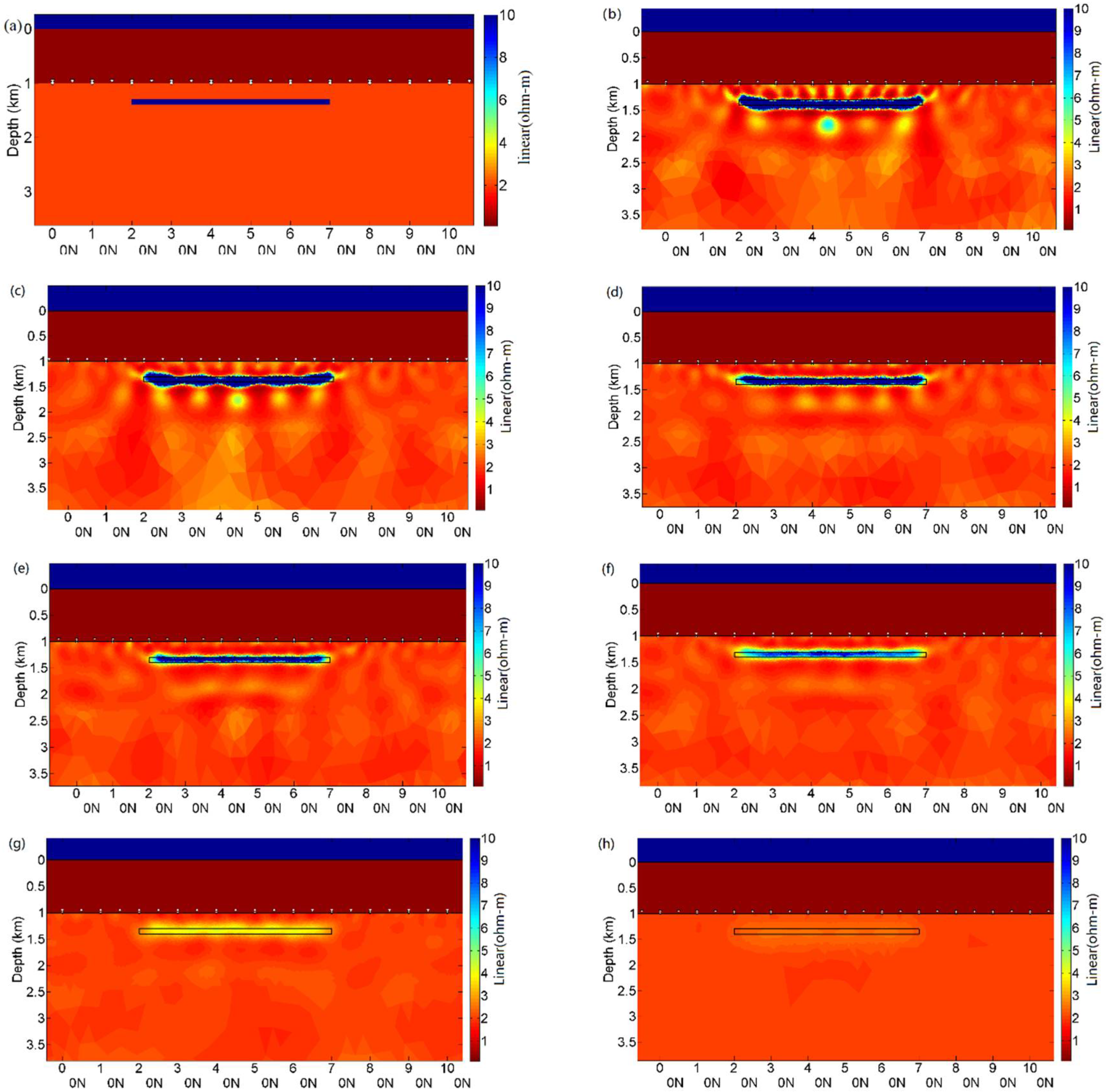
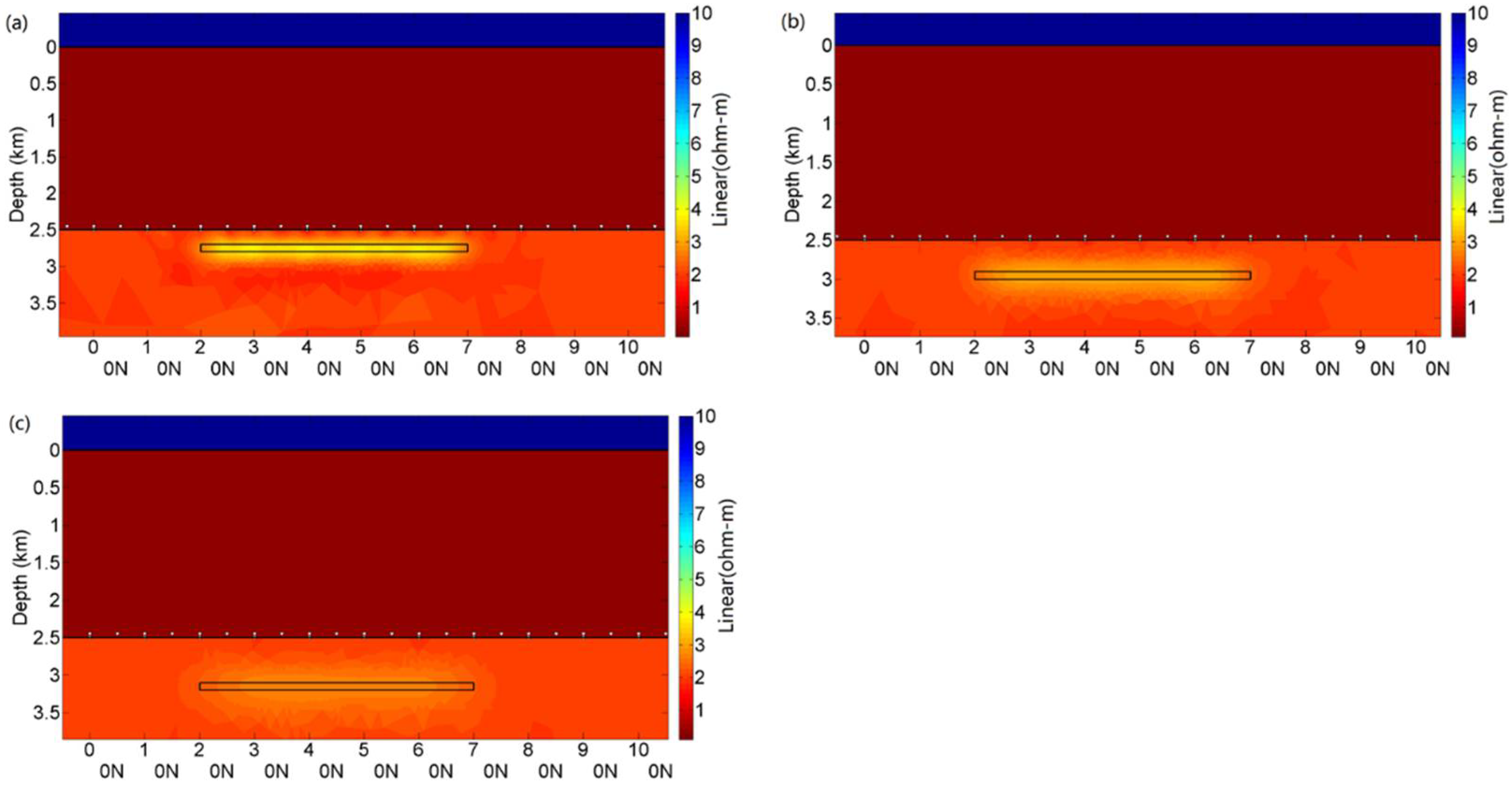
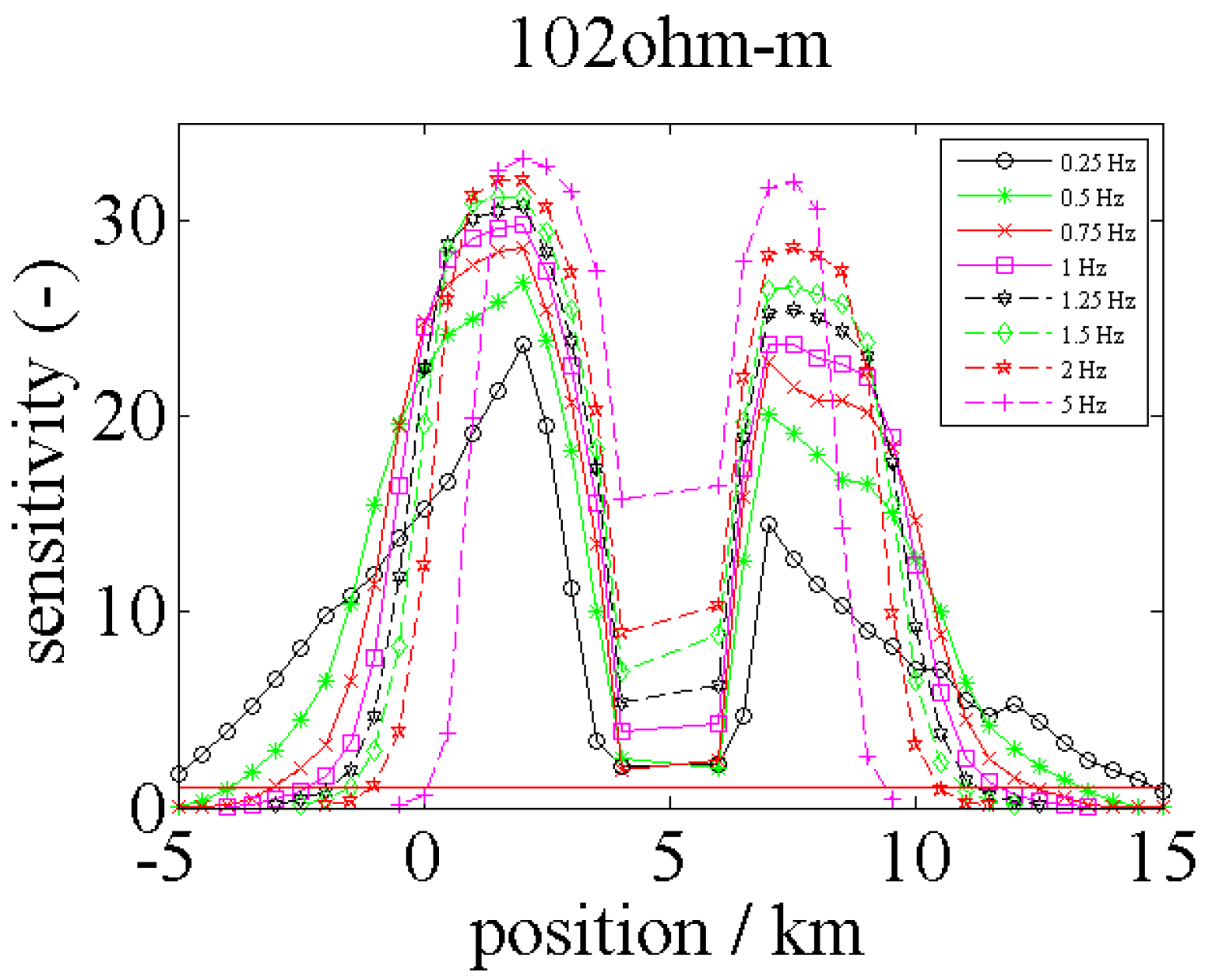
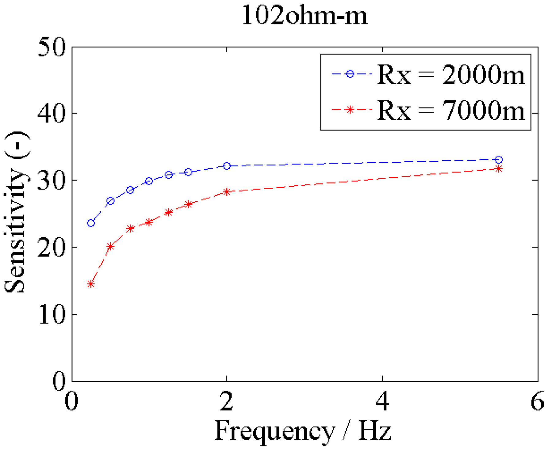
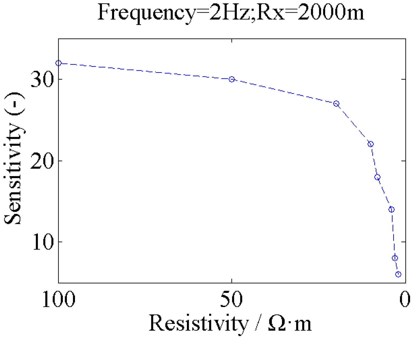
3. Results
4. Discussion and Conclusions
Author Contributions
Funding
Data Availability Statement
Acknowledgments
Conflicts of Interest
References
- Kvenvolden, K.A. Gas hydrates—Geological perspective and global change. Rev. Geophys. 1993, 31, 173–187. [Google Scholar] [CrossRef]
- Milkov, A.V.; Sassen, R. Economic geology of offshore gas hydrate accumulations and provinces. Marine Petr. Geol. 2002, 19, 1–11. [Google Scholar] [CrossRef]
- Sloan, E.D., Jr.; Koh, C.A. Clathrate Hydrates of Natural Gases; CRC Press: Boca Raton, FL, USA, 2007. [Google Scholar]
- Dawe, R.A.; Thomas, S. A large potential methane source—Natural gas hydrates. Energy Sour. Part A 2007, 29, 217–229. [Google Scholar] [CrossRef]
- Eidesmo, T.; Ellingsrud, S.; MacGregor, L.M.; Constable, S.; Sinha, M.C.; Johansen, S.E.; Kong, F.N.; Westerdah, H. Sea Bed Logging (SBL), a new method for remote and direct identification of hydrocarbon filled layers in deep-water areas. First Break 2002, 20, 144–152. [Google Scholar] [CrossRef]
- Johansen, S.E.; Amundsen, H.E.F.; Røsten, T.; Ellingsrud, S.; Eidesmo, T.; Bhuiyan, A.H. Subsurface hydrocarbons detected by electromagnetic sounding. First Break 2005, 23, 1–36. [Google Scholar] [CrossRef]
- Constable, S.; Weiss, C.J. Mapping thin resistors and hydrocarbons with marine EM methods: Insights from 1D modeling. Geophysics 2006, 71, G43–G51. [Google Scholar] [CrossRef]
- Constable, S.; Srnka, L.J. An introduction to marine controlled source electromagnetic methods for hydrocarbon exploration. Geophysics 2007, 72, WA3–WA12. [Google Scholar] [CrossRef]
- Evans, R.L.; Sinha, M.C.; Constable, S.C.; Unsworth, M.J. On the electrical nature of the axial melt zone at 13° N on the East Pacific Rise. J. Geophys. Res. Solid Earth 1994, 99, 577–588. [Google Scholar] [CrossRef]
- Macgregor, L.M.; Constable, S.; Sinha, M.C. The Ramesses experiment -III. Controlled source electromagnetic sounding of the Reykjanes Ridge at 57°45′ N. Geophys. J. Int. 1998, 135, 772–789. [Google Scholar] [CrossRef]
- Edwards, R.N. On the resource evaluation of marine gas hydrate deposits using sea -floor transient electric dipole-dipole methods. Geophysics 1997, 62, 63–74. [Google Scholar] [CrossRef]
- Marina, G.P.; Yuri, G.S.; Petr, A.D.; Denis, V.V.; Yulia, I.K. Electromagnetic field analysis in the marine CSEM detection of homogeneous and inhomogeneous hydrocarbon 3D reservoirs. J. Appl. Geophys. 2015, 119, 147–155. [Google Scholar] [CrossRef]
- Streich, R. Controlled-source electromagnetic approaches for hydrocarbon exploration and monitoring on land. Surv. Geophys. 2016, 37, 47–80. [Google Scholar] [CrossRef]
- Schwalenberg, K.; Engels, M.; Rippe, D.; Scholl, C. Marine CSEM for Gas Hydrate Exploration Using a Seafloor-towed Multi-receiver System. In Proceedings of the 76th EAGE Conference and Exhibition-Workshops, Amsterdam, The Netherlands, 16–19 June 2014; p. cp-401-00067. [Google Scholar] [CrossRef][Green Version]
- Schwalenberg, K.; Rippe, D.; Koch, S.; Scholl, C. Marine-controlled source electromagnetic study of methane seeps and gas hydrates at Opouawe Bank, Hikurangi Margin, New Zealand. J. Geophys. Res. Solid Earth 2017, 122, 3334–3350. [Google Scholar] [CrossRef]
- Chen, K.; Jing, J.E.; Zhao, Q.X.; Luo, X.H.; Tu, G.H.; Wang, M. Ocean bottom EM receiver and application for gas-hydrate detection. Chin. J. Geophys. 2017, 60, 4262–4272. (In Chinese) [Google Scholar]
- Tharimela, R.; Augustin, A.; Ketzer, M.; Cupertino, J.; Miller, D.; Viana, A.; Senger, K. 3D controlled-source electromagnetic imaging of gas hydrates: Insights from the Pelotas Basin offshore Brazil. Interpretation 2019, 7, SH111–SH131. [Google Scholar] [CrossRef]
- Weitemeyer, K.A. Marine Electromagnetic Methods for Gas Hydrate Characterization; University of California: San Diego, CA, USA, 2008. [Google Scholar]
- Edwards, R.N.; Nobes, D.C.; Gomez-Trevino, E. Offshore electrical exploration of sedimentary basins: The effects of anisotropy in horizontally isotropic, layered media. Geophysics 1984, 49, 566–576. [Google Scholar] [CrossRef]
- Rodi, W.L. A technique for improving the accuracy of finite element solutions for MT data. Geophys. J. Int. 1976, 44, 483–506. [Google Scholar] [CrossRef]
- Jupp, D.L.B.; Vozoff, K. Two-dimensional magnetotelluric inversio. Geophys. J. Int. 1977, 50, 333–352. [Google Scholar] [CrossRef]
- Farquharson, C.G.; Oldenburg, D.W. Approximate sensitivities for the electromagnetic inverse problem. Geophys. J. Int. 1996, 126, 235–252. [Google Scholar] [CrossRef][Green Version]
- McGillivray, P.R.; Oldenburg, D.W. Methods for calculating Fréchet derivatives and sensitivities for the non-linear inverse problem: A comparative study. Geophys. Prospect 1990, 38, 499–524. [Google Scholar] [CrossRef]
- McGillivray, P.R.; Oldenburg, D.W.; Ellis, R.G.; Habashy, T.M. Calculation of sensitivities for the frequency-domain electromagnetic problem. Geophys. J. Int. 1994, 116, 1–4. [Google Scholar] [CrossRef]
- Spies, B.R.; Habashy, T.M. Sensitivity analysis of crosswell electromagnetics. Geophysics 1995, 60, 834–845. [Google Scholar] [CrossRef]
- Gribenko, A.; Zhdanov, M. Rigorous 3D inversion of marine CSEM data based on the integral equation method. Geophysics 2007, 72, 540–552. [Google Scholar] [CrossRef]
- Kaputerko, A.; Gribenko, A.; Zhdanov, M. Sensitivity analysis of Marine CSEM surveys. In SEG Technical Program Expanded Abstracts; Society of Exploration Geophysicists (SEG): Houston, TX, USA, 2007; pp. 609–613. [Google Scholar] [CrossRef]
- Mittet, R.; Morten, J.P. The marine controlled-source electromagnetic method in shallow water. Geophysics 2013, 78, E67–E77. [Google Scholar] [CrossRef]
- Scholl, C.; Edwards, R.N. Marine downhole to seafloor dipole-dipole electromagnetic methods and the resolution of resistive targets. Geophysics 2007, 72, WA39–WA49. [Google Scholar] [CrossRef]
- Gao, G.; Alumbaugh, D.; Chen, J.; Eyl, K. Resolution and uncertainty analysis for marine CSEM and crosswell EM imagin. In SEG Technical Program Expanded Abstracts; Society of Exploration Geophysicists (SEG): Houston, TX, USA, 2007; Volume 27, pp. 623–627. [Google Scholar] [CrossRef]
- Morten, J.P.; Bjørke, A.K.; Nguyen, A.K. Hydrocarbon reservoir thickness resolution in 3D CSEM anisotropic inversion. In SEG Technical Program Expanded Abstracts 2010; Society of Exploration Geophysicists: Tulsa, OK, USA, 2010; pp. 599–603. [Google Scholar] [CrossRef]
- Brown, V.; Hoversten, M.; Key, K.; Chen, J. Resolution of reservoir scale electrical anisotropy from marine CSEM data. Geophysics 2011, 77, 147. [Google Scholar] [CrossRef][Green Version]
- Moghadas, D.; Engels, M.; Gehrmann, R.A.S.; Schwalenberg, K. 3D numerical modelling and 1D inversion and resolution analysis of time-domain marine controlled source electromagnetic data. In Proceedings of the Schmucker Weidelt Kolloquium, Elektromagnetische Tiefenforschung, Kirchhundem-Rahrbach, Germany, 23–27 September 2013; pp. 104–108. [Google Scholar]
- Sasaki, Y. Resolution of shallow and deep marine CSEM data inferred from anisotropic 3D inversion. In SEG Technical Program Expanded Abstracts; Society of Exploration Geophysicists (SEG): Houston, TX, USA, 2013. [Google Scholar] [CrossRef]
- Blatter, D.; Key, K.; Ray, A.; Gustafson, C. Bayesian Joint Inversion of Surface-Towed CSEM and MT Data: Quantifying the Resolution Gain. In Proceedings of the 24th EM induction Workshop, Helsingør, Denmark, 12–19 August 2018. [Google Scholar]
- Ren, Z.; Kalscheuer, T. Uncertainty and resolution analysis of 2D and 3D inversion models computed from geophysical electromagnetic data. Surv. Geophys. 2020, 41, 47–112. [Google Scholar] [CrossRef]
- Lee, M.W.; Collett, T.S. Scale-dependent gas hydrate saturation estimates in sand reservoirs in the Ulleung Basin, East Sea of Korea. Marine Petr. Geol. 2013, 47, 195–203. [Google Scholar] [CrossRef]
- Key, K. MARE2DEM: A 2-D inversion code for controlled-source electromagnetic and magnetotelluric data. Geophys. J. Int. 2016, 207, 571–588. [Google Scholar] [CrossRef]
- Matsumoto, R.; Takedomi, Y.; Wassada, H. Exploration of marine gas hydrates in Nankai Trough, offshore Central Japan. In Proceedings of the AAPG Annual Convention, Denver, CO, USA, 3–6 June 2001; Volume 36. [Google Scholar]


| Resistivity (Ω·m) | Thickness (m) | Length (m) | |
|---|---|---|---|
| Air | 1013 | ||
| Sea Water | 0.3 | 1000 | |
| Target | 102, 52, 22, 12, 10, 6, 5, 4 | 100 | 5000 |
| Sediments | 2 |
Publisher’s Note: MDPI stays neutral with regard to jurisdictional claims in published maps and institutional affiliations. |
© 2021 by the authors. Licensee MDPI, Basel, Switzerland. This article is an open access article distributed under the terms and conditions of the Creative Commons Attribution (CC BY) license (https://creativecommons.org/licenses/by/4.0/).
Share and Cite
Guo, Z.; Yuan, Y.; Jiang, M.; Liu, J.; Wang, X.; Wang, B. Sensitivity and Resolution of Controlled-Source Electromagnetic Method for Gas Hydrate Stable Zone. Energies 2021, 14, 8318. https://doi.org/10.3390/en14248318
Guo Z, Yuan Y, Jiang M, Liu J, Wang X, Wang B. Sensitivity and Resolution of Controlled-Source Electromagnetic Method for Gas Hydrate Stable Zone. Energies. 2021; 14(24):8318. https://doi.org/10.3390/en14248318
Chicago/Turabian StyleGuo, Zhenwei, Yunxi Yuan, Mengyuan Jiang, Jianxin Liu, Xianying Wang, and Bochen Wang. 2021. "Sensitivity and Resolution of Controlled-Source Electromagnetic Method for Gas Hydrate Stable Zone" Energies 14, no. 24: 8318. https://doi.org/10.3390/en14248318
APA StyleGuo, Z., Yuan, Y., Jiang, M., Liu, J., Wang, X., & Wang, B. (2021). Sensitivity and Resolution of Controlled-Source Electromagnetic Method for Gas Hydrate Stable Zone. Energies, 14(24), 8318. https://doi.org/10.3390/en14248318