Article

Method for Designing Robust and Energy Efficient Railway Schedules

by
Franciszek Restel
1,*,
Łukasz Wolniewicz
1 and
Matea Mikulčić
2
1
Department of Technical Systems Operation and Maintenance, Faculty of Mechanical Engineering, Wroclaw University of Science and Technology, 50-370 Wroclaw, Poland
2
Department of Railway Transport, Faculty of Transport and Traffic Sciences, University of Zagreb, 10000 Zagreb, Croatia
*
Author to whom correspondence should be addressed.
Energies 2021, 14(24), 8248; https://doi.org/10.3390/en14248248
Submission received: 15 November 2021 / Revised: 1 December 2021 / Accepted: 5 December 2021 / Published: 8 December 2021

Abstract

:
The robustness of the timetable is a sensitive issue in the daily realization of railway operations. As shown in the paper, robustness is a function of time reserves that helps to prevent unscheduled stops resulting from traffic disruptions and causing a higher energy consumption. The correct handling of time reserves while scheduling is a multidimensional issue, and it has a significant influence on the energy consumption of railway traffic. Therefore, the paper aims to show a simulation-based method, taking into account failure occurring probabilities and their consequences to get an acceptable level of robustness, that can be quantified by the probability of no delay propagation. This paper presents a method for the addition of time margins to the railway timetable. The iterative time buffer adding method is based on operational data as a knowledge source, to achieve the punctuality target. It was verified on a real railway line. An analysis of energy consumption for unscheduled train stops depending on the added buffer time was conducted after the literature review and the presentation of the evaluation model. The paper ends with discussion of the results and conclusions.

1. Introduction

Increasing the level of services provided by rail carriers is related to minimizing delays. Robust schedules allow for this. The causes of delays may be, among others, repair works, rolling stock and infrastructure failures, inappropriate fulfilment of duties by the staff, extended detention time at the station, as well as the propagation of secondary delays. Additionally, unplanned train stops result in increased energy consumption [1].
Each disruption can lead to delays and unplanned stops. Thus, a robust timetable preventing delay propagation should cause energy savings.
Increasing time reserves also increases robustness but decreases network capacity. Scheduling should be designed to make the best use of people and equipment time, the capacity of railroads used by different carriers, and the robustness of the rail transportation system to disruptions.
It follows the papers aim to elaborate a new simulation-based method supported by a probabilistic approach for developing robust timetables, obtaining a significant energy saving. The robustness of a timetable depends on time margins; therefore, the subject of the method is to assign time reserves.

2. Literature Review

In recent years, it has been increasingly proposed to attempt to rationalize the energy consumption of a vehicle or group of vehicles by undertaking any initiatives to reduce energy consumption by rail transport. This is mainly related to the higher energy demand of new vehicles [2,3,4]. The issues related to adverse events and their impact are related to the analysis of the entire system and not only a single vehicle. The necessity of considering the energy consumption of the entire system, and not only parts of it, is indicated by articles [5,6,7,8]. The proposals described so far concern, however, either an isolated, small fragment of the railway system, e.g., the [5,6,8] subway line, a local railway line [9] (with little possibility of modifying the timetable) or consider the case of specific trains [10] or the interaction of a pair of vehicles [1,8,11]. Optimization of the timetable to minimize energy demand while maintaining the capacity of the railway infrastructure has been analyzed in [8]. In work, attention was paid to introducing a correction to the shape of the train’s running curves, recovering energy from braking and storing it in a vehicle or transferring it to another vehicle in the system. The use of unoccupied capacity on the metro line network resulted in an increase in the reduction of energy consumption from 9.13% to 10.66%. In the rationalization of energy demand and simultaneous introduction of construction changes in the timetable, savings of 7.23% to even 24.34% were achieved in [1]. The two-object integer programming model proposed in [12] allows the optimization of schedules in terms of energy consumption and quality of service. The applied genetic algorithm with binary coding allows the control of stop and go times. The paper [13] presents coasting control methods using genetic algorithms. It reduces energy consumption and travel time. In [14], a model using nonlinear programming for trajectory analysis was shown. In [15], the optimization model includes passenger travel time and energy consumption to find the best trajectory under given conditions. In [16,17], algorithms were used to optimize energy consumption. The method proposed in [18] for recovering train traffic after unwanted events consisted of network optimization models for operational sections in the railroad network and it is structured as a series of “what-if” scenarios.
As crucial for future exploitation of available railway infrastructure with the variability of operating conditions, railway timetable planning and its robustness have been challenging research areas for many years. Some studies are dedicated to different kinds of disturbances and consequent delays, their characteristics, effects, and transmission among railway operational flow [19,20,21,22,23,24]. Others tend to study robustness indicators and measures, evaluate timetable robustness or explore ways of its improvement concerning one or multiple selected robustness measures and types of the timetable at various levels of detail [25,26,27,28,29,30]. For more prominent disturbances that cannot be mitigated or eliminated by good planning in the design phase, the critical role has predictive and real-time disruption management with effective recovery strategies and integrated decision-making on retiming, reordering or rerouting trains to avoid conflicts, especially in case of lack of infrastructure capacity. Although not directly relevant for this paper, more about disruption management practices in European countries can be seen in [31].
The literature offers various definitions of robustness related to components of the rail transport system, among other things:
  • Unexpected problems can be dealt with without significant schedule modifications [32];
  • The schedule is robust when delays from one period do not spread to the next [33];
  • The ability of a schedule to resist design errors, changes in parameters and operating conditions [34].
Moreover, robustness measures can be related to timetable characteristics (ex-ante) or executed traffic performance (ex-post) [35]. Measures from the first-mentioned category assume sizing and allocation of running time supplement, buffer time or dwell time in the timetable or decrease of traffic heterogeneity via train reorder, unification of average speed or some other beneficial strategies (i.e., skip-stopping, holding trains and reserving rolling stock). On the other side, traffic performance measures are based on punctuality, delays, the number of violated connections or the number of trains being on time to a station. To guarantee punctual train running, in this paper, an analysis is carried out to assign buffer times to the timetable using real disturbance data as an example.
To compute the buffer times under the assumption of unknown and known distribution functions of disturbances, Shafia et al. [36] used a robust mixed-integer approach. Vansteenwegen and Oudheusden [37] used calculated ideal buffer values for linear programming improvement of cyclic passenger timetables with respect to minimized generalized waiting costs. Kroon et al. [38] developed a stochastic optimization model for optimal allocation of running time supplements and buffer times.
Conversely, in Andersson et al. [25], buffer time allocation is connected to delay-sensitive critical points, characterized by immediate successive departures and overtaking. Reallocation of existing runtime and headway margins in the timetable to such defined critical points with mixed-integer linear programming reduced delays [39]. Lee et al. [40] performed reallocation of time supplements and buffer times of the original aperiodic passenger timetable with heuristics based on simulation. They pointed out that manipulating with time supplement is more effective for reducing system delay in a busy railway system with a dense timetable than adjusting buffer time. Meng et al. [41] incorporated another heuristic technique known as critical time allocation to minimize the sum of train delays in the event of operational disturbances. Although keeping the same headway value and train order, reallocated headway buffers and running time supplements showed limited improvements after a certain amount of delay, and in case that, all trains have the same speeds and homogeneous characteristics.
Khoshniyat and Peterson tested [42] a concept of travel time-dependent reserved minimum headways with modified buffer times in aperiodic timetables by taking into account uncertainty of train arrival times and stations capacity. Huang et al. [43] incorporated real-world train operation data in buffer time allocation procedure for sections and stations to increase timetable robustness without capacity loss and better recover from delays. Yang et al. [44] suggested buffer time allocation at stations based on the impact of delay on trains by integrating the operational performance data in their model of delay time distribution. Burggraeve and Vansteenwegen [45] focused on the optimal buffer and running time calculation regarding conflict-free routing plans and allocation, which brings the shortest total passenger travel time for cyclic timetables with optimal infrastructure usage. Moreover, while optimizing the station capacity utilization, Yuan and Hansen [46] showed exponential relation between the size of buffer time between train paths at level crossings and the average knock-on delay of all trains. The same authors later [47] improved the optimal allocation of buffer times at railway bottlenecks such as stations and junctions to minimize weighted knock-on delays. Another example of reallocation of existing buffer times with respect to capacity constraints of lines and delay propagation to/from all events on the single- or double-track corridor in the considered time window is presented in [48].
Most models from the literature involve analytical or simulation approaches for buffer time allocation. However, there is a lack of methods focused on robustness, which can be understood as the probability of no delay propagation after an unwanted event. Moreover, the probability distribution is mainly related to a specified process and is dependent on its duration. Thus, for the approaches, it is necessary to get many different distributions.

3. Time Margins Development Method

This section explores the use of time margins to improve robustness and decrease energy consumption. Time margins are understood as time values added to processes to be buffered for unexpected disruptions. More closely to operational robustness, that is, a process quality related to processes implemented by the system. It is the ability of the timetable not to include disruptions of system unavailability to the operation process. Thus, a totally operational robust system will have no disruptions in the implementation. Moreover, the operational robustness does not allow reconfiguration. In practice, full operational robustness is not available. Reaching such a level would cause high time margins that would be unreasonable due to a significant capacity loss.
First, for the method, the real system for which the rail network model will be built is observed. This observation consists of identifying the railroad line and train kilometre points for which event data will be collected and determining the scope of the analysis. Delay models are built in terms of track infrastructure, station layout, kilometers, and track layout and control system data are used. The process randomness of the input for the simulation is described by the operation time between failures distribution and the distribution of delays resulting from the failures (Figure 1).
The data sample for the times between failures (TBF) based on 163 undesirable events registered for a real railway line in Poland. The TBFs were calculated as the time interval between two failures, expressed not in absolute time but in the time when the train was operated. Six trains launched every day (three reagional and three express) have been investigated for a period of 3 months, to get the data. The data sample for the delay times was also gathered for the same railway line and the same time period, but for 24 trains. In total 777 undesirable events were registered.
According to the gathered data sample, the Weibull distribution Wei (0.598; 195.348) was proposed to model the times between failures. Using the Kolmogorov test at a significance level of 0.05, it was proven that the Wei (0.598; 195.348) distribution fits the random variable.
For the delays, the Lognormal distribution LN (1.498; 0.959) was proposed. Using the same statistical test, it was proven that it fits the variable. The presented distributions are true for the boundary conditions of the analyzed railway line. Thus, the installed traffic control device type, the type of trains and passengers, the type of superstructure as well as the environmental influence. Then, the trains are defined within their most important deterministic parameters (weight, length, power supply, installed power) as well as random characteristics (time between failures distribution and delay time distribution).
The next point is to add the desired timetable in basic form without time margins. For the next step, the control points have to be established, where the delays will be analyzed. Thus, sections will be created to which reserves will be allocated for moving trains.
The preparation phase is finished, and the simulation can be run for a certain number of experiments (e.g., n = 100). After the simulation, the cumulated distribution functions for the delays on each evaluation section are calculated separately for each direction. The simulation process used for the evaluation process is shown in Figure 2. The diagram starts with the departure of the train from the station and ends with the arrival of the train at the station, including the stopping time. The generation of undesirable events at the station and on the route is considered. In the first instance, an event can be generated while the train is moving. Then the train stops for the duration of the event. If the event is generated on a station, the train stops for the duration of the event. Events are generated from probability density distributions assigned to trains according to the example from Figure 1.
Separate probability distributions are for the times between events and the duration of the event. The output information of the simulation model of railway operation processes is operational robustness. It can be estimated basically for a given pair of processes, as the probability that the first one will end before the second one has to start. The probability will be calculated as the integral of the probability density function of the ending time deviations from zero to the time-space value between the processes. Thus:
O R o ω α = P r ( T α T ω α ) = F α ( T ω α ) = 0 T ω α f α ( T α ) d ( T α )
where:
O R o ω α —operational robustness for processes α and ω ;
P r ( T α T ω α ) —probability that the time deviation T α of process α from the shortest implementation time m i n T α d u r will be not higher than the scheduled time-space T ω α to process ω ;
f α ( T α ) —probability distribution of the time deviation T α of process α from the shortest implementation time m i n T α d u r ;
F α ( T ω α ) —cumulated distribution function for T α = T ω α , for the distribution f α ( T α ) .
After the results are available, each section has to be evaluated in terms of the occurred delays. According to the publication [49], the border value was chosen, that 95% of all delays must be not greater than 2.5 min. Therefore, it will be proven for each section, and if necessary, cumulated distribution functions of delays for each train type on the given section will be elaborated. Using them, time margins will be added, taking the ninth decile of primary delays.
When the time margins are added for all trains on all sections, the simulation will be run again, and time margins will be added again according to the previous steps. It will be done till the condition of 95% delays not greater than 2.5 min will be reached. Figure 3 shows a flowchart of the time margin elaboration model.
This process continues until a satisfactory punctuality level is reached. When this level is satisfied, the timetable is approved, and any further changes are terminated.

4. Case Description

The case study stage presented here replicates conditions from the railroad on which the data were collected. Each route is characterized by different factors affecting incidents. In our case, there is a homogeneous traffic structure—passenger trains, electric traction. All regional trains are served by the same type of train set. The express trains also have a homogenous structure in terms of the type of locomotives with the same number of cars. A relay traffic control system was used. The line is 82 km long, and there are 7 traffic stations on it. The average distance between the stations is 22 km.
The reliability characteristics in terms of delay distribution and time between failure distribution are the same for both train types. The model of the fragment of a railroad line (Figure 4) was built in OpenTrack that is common used simulation program for railway networks. The model representsa real regional route in Poland with high traffic intensity. The travel time results for the trains and the solution of the equation of motion were verified. They coincide with the mathematical model implemented in the MATLAB environment. The error of calculating the travel time is no more than 1%.
In the chosen section, there is a uniform traffic structure—passenger transport. Trains run in two directions. The section includes six stations (four on the mainline (A, C, D, E) and two on the sideline (X, Z)). There is one branch station on the route (p.odg. B), from which it is possible to access the sideline. The sideline connects to the mainline in the area of station E. The length of the analyzed route is 82 km.
The mainline is double track, electrified, with speed limited to 120 km/h, while the sideline is single track, electrified, with a maximum speed of 120 km/h. Within stations X and Z it is possible for trains coming from opposite directions to pass each other. The characteristics of each station in terms of the number of tracks and platforms are as follows (Table 1).
The section under study uses a relay traffic control system. Therefore, the mainline is divided into four intervals and the sideline into three. The train traffic volume during the considered time interval 04:00 a.m.–04:00 p.m. is 10 pairs of trains on the mainline and 5 pairs of trains on the sideline. A traffic peak is observed between 06:00–9:00 a.m. in the morning and 02:00–04:00 p.m. in the afternoon. The capacity of the mainline is utilized at 85% and the sideline at 94%. The mainline is only used by fast trains (travel time 43 min), while the sideline is used by regional trains (travel time 55 min). The model of the analyzed railroad line in the simulation program is shown in Figure 4. The fast train stops at each station are 1 min long, and the regional train stops are 2 min. Fast trains are composed of one locomotive of the Polish type EU07 and six-passenger coaches. At the same time, the regional trains are operated by electric multiple units of the Polish type 45We, consisting of six coaches.
The primary timetable does not include buffer times. Station breaks are used for passenger exchange, and a train can’t depart earlier than the scheduled stop time. For each train along the entire route, section reservation and section release times (blocking start and end times) are provided. This is important because of the railroad traffic control system used, which affects the line’s capacity. The specificity of its operation requires observing the reservation of successive intervals occupied by the train during the simulation. The interval release time for the next train was assumed as 1 min.
For the analyzed case, two train types have been implemented. The energy consumption for the acceleration process was calculated for both, according to Newton’s second law of dynamics described by the equation [50]:
F ( v , x ) = m · k · d 2 x d t 2  
The results are shown in Table 2. The increased energy consumption resulting from an unplanned stop is obtained by subtracting the energy required to travel the given distance at a constant speed from the acceleration energy.
Thus, the total energy loss due to delays will be the number of unscheduled stops multiplied by the increased energy consumption for the given train type.
The presented approach was tested using a railway line with homogenous regional traffic and conditions described in the next section. The times between failures (TBF) and the delay values have been analyzed for such conditions represented on a real Polish railway line. The empirical distributions are shown in Figure 1.

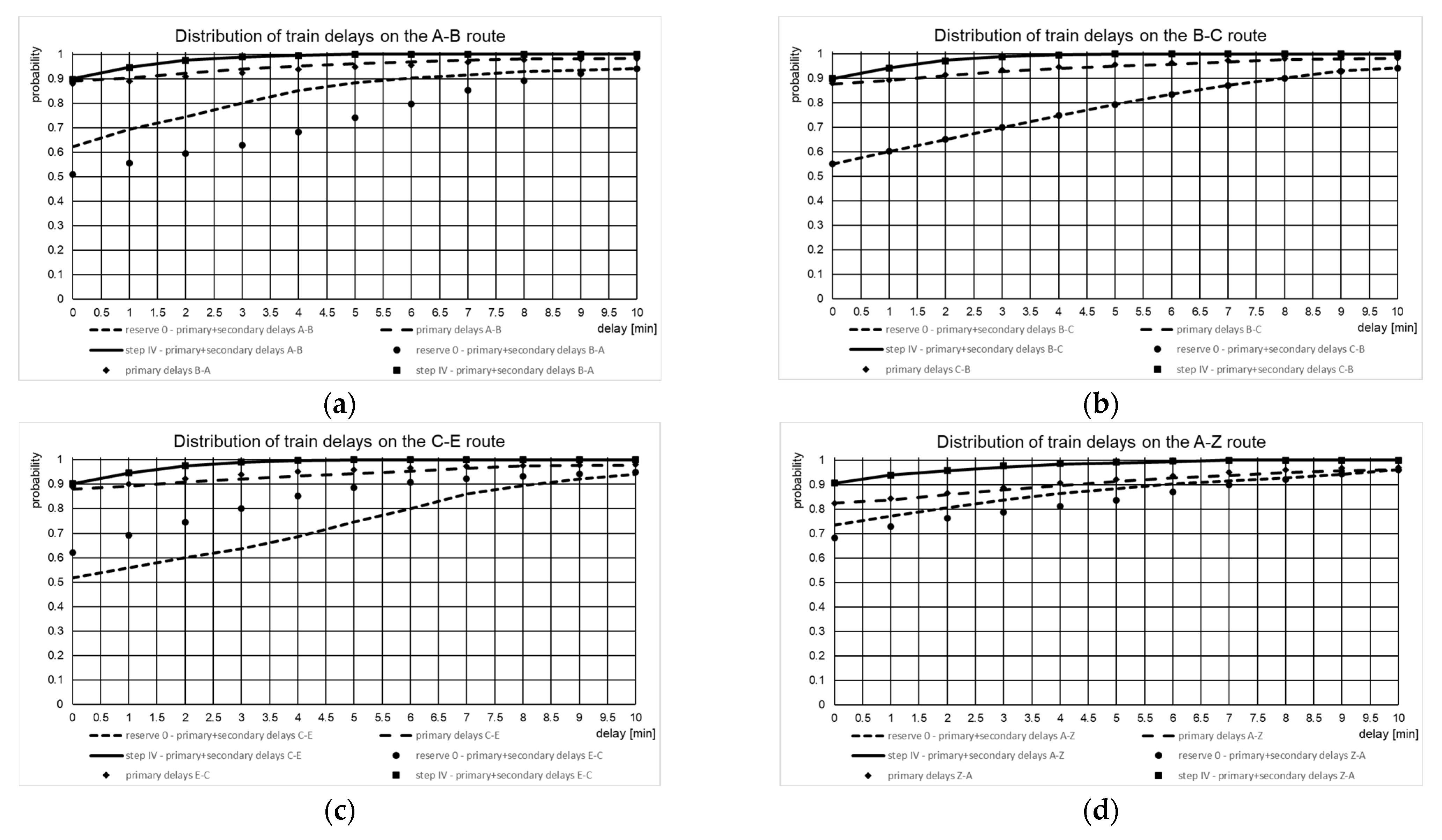
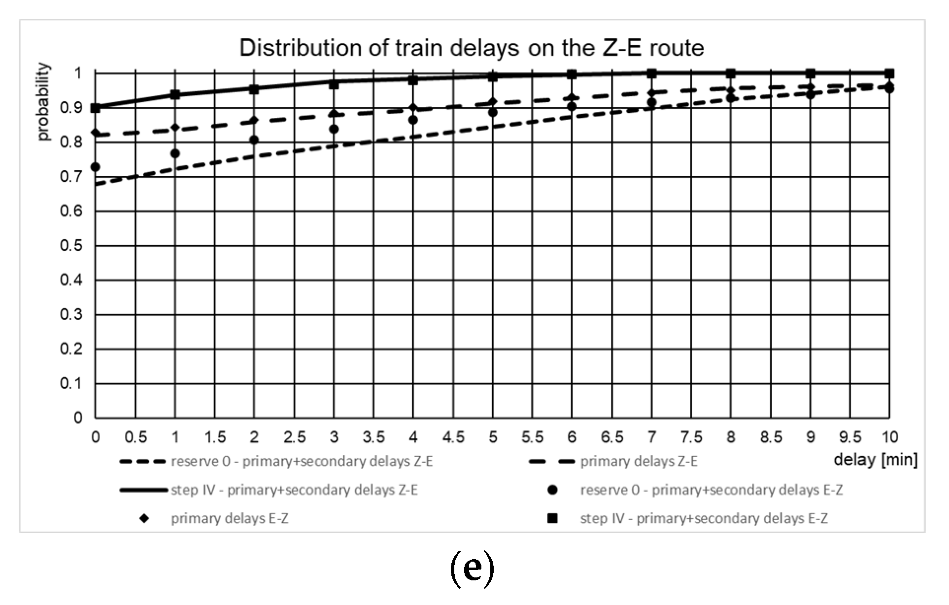
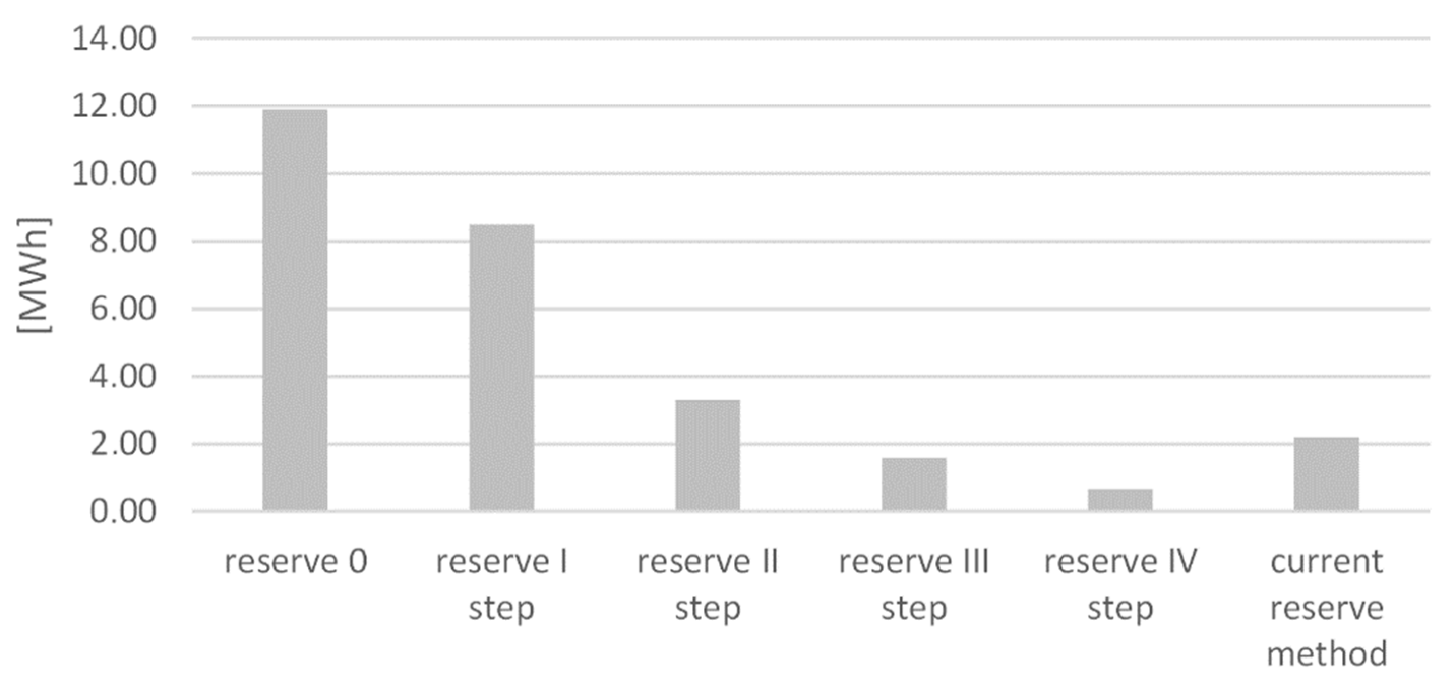
5. Discussion of Results

Figure 5 shows the results of the train delay distributions for each section, excluding the punctual trains. The results show the primary delays and the primary and secondary delays for reserve 0 and reserve IV.
In the method used in this paper, at the beginning short buffer were added to the schedule without buffer times. Then a simulation was run. The delay results from this simulation were manually checked. The assumed level of punctuality was not achieved. The buffers were gradually increased for individual trains, and further simulations were run. In total, four iterations of adding buffers were performed to achieve 90% punctuality in train running. The results after adding each buffer level are shown in Table 3 for both directions on each section. Table 4 shows the average number of unscheduled train stops per 12 h of simulation.
Punctuality results for the A–E and E–A double-track line are better than for the A–E–X and E–X–A single-track line. This is due to the interaction of trains when entering the area of station A and station E on the double-track line. For trains on the A–E and E–A line, maximum delay values of 5 min and 90% on-time trains were obtained, and for the A–E–X and E–X–A line, maximum delay values of 7 min and 90% on-time trains were obtained.
The primary energy losses due to undesirable train stops caused by traffic disruptions are about 11.90 MWh for the analyzed case. The value is valid for no time margins in the schedule. After adding the first time margins, the energy losses were reduced to 8.49 MWh (Figure 6). The following method steps gave more significant savings till its last stage, where 0.66 MWh were reached. While the current time margin adding method results in an increased energy consuption by 2.19 MWh.

6. Conclusions

The proposed method quickly solves the problem of calculating buffers time adapted to events occurring on the railroad network. Carrying out successive iterations and simulations with undesirable events guarantees the construction of a timetable robust to disturbances. As a consequence, the energy losses in the system are minimized.
Obtained punctuality on the level of 90% and delay not exceeding 2.5 min on the level of 95% is attractive for passengers of railroad transport. Moreover, the energy losses can be limited by using the proposed method to 6% about the fundamental value of 11.90 MWh without time reserves, and 30% in relation to the current method.
The method allows using data collected already in the system to allocate time reserves concerning operational experience where they are needed. Thus, the capacity losses are kept on a low level, and punctuality and connected energy losses are also minimized.
Further research should focus on integrating available databases and the automatization of the time margin addition method. As a result, a system should be developed for supporting the designing process of timetables. Not all events can be covered by the method. Therefore the follow-up actions will consider the management of disrupted traffic.

Author Contributions

Conceptualization, F.R., Ł.W. and M.M.; Methodology, F.R., Ł.W. and M.M.; Resources, F.R., Ł.W. and M.M.; Writing—Original Draft, F.R., Ł.W. and M.M. All authors have read and agreed to the published version of the manuscript.

Funding

This research received no external funding.

Institutional Review Board Statement

Not applicable.

Informed Consent Statement

Not applicable.

Data Availability Statement

Not applicable.

Conflicts of Interest

The authors declare no conflict of interest.

References

  1. Wang, P.; Goverde, R.M. Multi-train trajectory optimization for energy-efficient timetabling. Eur. J. Oper. Res. 2019, 272, 621–635. [Google Scholar] [CrossRef]
  2. Tian, Z.; Zhao, N.; Hillmansen, S.; Su, S.; Wen, C. Traction Power Substation Load Analysis with Various Train Operating Styles and Substation Fault Modes. Energies 2020, 13, 2788. [Google Scholar] [CrossRef]
  3. Pröhl, L.; Aschemann, H.; Palacin, R. The Influence of Operating Strategies regarding an Energy Optimized Driving Style for Electrically Driven Railway Vehicles. Energies 2021, 14, 583. [Google Scholar] [CrossRef]
  4. Cunillera, A.; Fernández-Rodríguez, A.; Cucala, A.P.; Fernández-Cardador, A.; Falvo, M.C. Assessment of the Worthwhileness of Efficient Driving in Railway Systems with High-Receptivity Power Supplies. Energies 2020, 13, 1836. [Google Scholar] [CrossRef]
  5. Zhao, N.; Roberts, C.; Hillmansen, S.; Tian, Z.; Weston, P.; Chen, L. An integrated metro operation optimization to minimize energy consumption. Transp. Res. Part C 2017, 75, 168–182. [Google Scholar] [CrossRef] [Green Version]
  6. Yang, X.; Chen, A.; Ning, B.; Tang, T. A stochastic model for the integrated optimization on metro timetable and speed profile with uncertain train mass. Transp. Res. Part B 2016, 91, 424–445. [Google Scholar] [CrossRef]
  7. González-Gil, A.; Palacin, R.; Batty, P.; Powell, J.P. A systems approach to reduce urban rail energy consumption. Energy Convers. Manag. 2014, 80, 509–524. [Google Scholar] [CrossRef] [Green Version]
  8. Huang, Y.; Yang, L.; Tang, T.; Gao, Z.; Cao, F.; Li, K. Train speed profile optimization with on-board energy storage devices: A dynamic programming based approach. Comput. Ind. Eng. 2018, 126, 149–164. [Google Scholar] [CrossRef]
  9. Gerben, M.; Scheepmaker, R.; Goverde, M.P. The interplay between energy-efficient train control and scheduled running time supplements. J. Rail Transp. Plan. Manag. 2015, 5, 225–239. [Google Scholar] [CrossRef]
  10. Kwaśnikowski, J. Elementy Teorii Ruchu i Racjonalizacja Prowadzenia Pociągu; Naukowe Instytutu Technologii Eksploatacji—PIB: Radom, Poland, 2013. [Google Scholar]
  11. Wang, P.; Goverde, M.P. Two-Train Trajectory Optimization with a Green-Wave Policy. Transp. Res. Rec. Transp. Res. Board 2016, 2546, 112–120. [Google Scholar] [CrossRef]
  12. Yang, X.; Ning, B.; Li, X.; Tang, T. A two-objective timetable optimization model in subway systems. IEEE Trans. Intell. Transp. Syst. 2014, 15, 1913–1921. [Google Scholar] [CrossRef]
  13. Yang, L.X.; Li, K.P.; Gao, Z.Y.; Li, X. Optimizing trains movement on a railway network. Omega 2012, 40, 619–633. [Google Scholar] [CrossRef]
  14. Gu, Q.; Tang, T.; Cao, F.; Song, Y.D. Energy-efficient train operation in urban rail transit using real-time traffic information. IEEE Trans. Intell. Transp. Syst. 2014, 15, 1216–1233. [Google Scholar] [CrossRef]
  15. ShangGuan, W.; Yan, X.H.; Cai, B.G.; Wang, J. Multiobjective optimization for train speed trajectory in CTCS high-speed railway with hybrid evolutionary algorithm. IEEE Trans. Intell. Transp. Syst. 2015, 16, 2215–2225. [Google Scholar] [CrossRef]
  16. Ke, B.R.; Lin, C.L.; Yang, C.C. Optimization of train energy-efficient operation for mass rapid transit systems. IET Intell. Transp. Syst. 2012, 6, 58–66. [Google Scholar] [CrossRef]
  17. Lu, S.; Hillmansen, S.; Ho, T.K.; Roberts, C. Single-train trajectory optimization. IEEE Trans. Intell. Transp. Syst. 2013, 14, 743–750. [Google Scholar] [CrossRef]
  18. Azad, N.; Hassini, E.; Verma, M. Disruption risk management in railroad networks: An optimization-based methodology and a case study. Transp. Res. Part B 2016, 85, 70–88. [Google Scholar] [CrossRef]
  19. Wen, C.; Li, Z.; Lessan, J.; Fu, L.; Huang, P.; Jiang, C. Statistical investigation on train primary delay based on real records: Evidence from Wuhan–Guangzhou HSR. Int. J. Rail Transp. 2017, 5, 170–189. [Google Scholar] [CrossRef]
  20. Roßler, D.; Reisch, J.; Hauck, F.; Kliewer, N. Discerning Primary and Secondary Delays in Railway Networks using Explainable A.I. In Transportation Research Procedia; Elsevier: Amsterdam, The Netherslands, 2021; pp. 171–178. [Google Scholar] [CrossRef]
  21. Goverde, M.P. A delay propagation algorithm for large-scale railway traffic networks. Transp. Res. Part C Emerg. Technol. 2010, 18, 269–287. [Google Scholar] [CrossRef]
  22. Büker, T.; Seybold, B. Stochastic modelling of delay propagation in large networks. J. Rail Transp. Plan. Manag. 2012, 2, 34–50. [Google Scholar] [CrossRef]
  23. Şahin, İ. Markov chain model for delay distribution in train schedules: Assessing the effectiveness of time allowances. J. Rail Transp. Plan. Manag. 2017, 7, 101–113. [Google Scholar] [CrossRef]
  24. Vromans, M.J.C.M.; Dekker, R.; Kroon, L.G. Reliability and heterogeneity of railway services. Eur J. Oper. Res. 2006, 172, 647–665. [Google Scholar] [CrossRef]
  25. Andersson, E.V.; Peterson, A.; Törnquist, J. Quantifying railway timetable robustness in critical points. J. Rail Transp. Plan. Manag. 2014, 3, 95–110. [Google Scholar] [CrossRef] [Green Version]
  26. Salido, M.; Barber, F.; Ingolotti, L. Robustness in railway transportation scheduling. In Proceedings of the 2008 7th World Congress on Intelligent Control and Automation, Chongqing, China, 25–27 June 2008; pp. 2880–2885. [Google Scholar]
  27. Salido, M.A.; Barber, F.; Ingolotti, L. Robustness for a single railway line: Analytical and simulation methods. Expert Syst. Appl. 2012, 39, 13305–13327. [Google Scholar] [CrossRef] [Green Version]
  28. Cerreto, F. Micro-simulation based analysis of railway lines robustness. In Proceedings of the 6th International Conference on Railway Operations Modelling and Analysis, Tokyo, Japan, 23–26 March 2015. [Google Scholar]
  29. Corman, F.; D’Ariano, A.; Hansen, I.A. Evaluating disturbance robustness of railway schedules. J. Intell. Transp. Syst. 2014, 18, 106–120. [Google Scholar] [CrossRef]
  30. Cacchiani, V.; Toth, P. Robust Train Timetabling. In Handbook of Optimization in the Railway Industry; International Series in Operations Research and Management Science 268; Springer: New York, NY, USA, 2018; pp. 93–115. [Google Scholar] [CrossRef]
  31. Schipper, D.; Gerrits, L. Differences and similarities in European railway disruption management practices. J. Rail Transp. Plan. Manag. 2018, 8, 42–55. [Google Scholar] [CrossRef]
  32. Takeuchi, Y.; Tomii, N. Robustness indices for train rescheduling. In Proceedings of the CDROM Proceedings of the 1st International Seminar on Railway Operations Modelling and Analysis, Delft, The Nethrlands, 7–9 June 2005. [Google Scholar]
  33. Goverde, R.M.P. Railway timetable stability analysis using max-plus system theory. Transp. Res. Part B Methodol. 2007, 41, 179–201. [Google Scholar] [CrossRef]
  34. Bešinović, N.; Goverde, R.M.P.; Quaglietta, E.; Roberti, R. An integrated micro-macro approach to robust railway timetabling. Transp. Res. Part B Methodol. 2016, 87, 14–32. [Google Scholar] [CrossRef] [Green Version]
  35. Andersson, E.V. Assessment of Robustness in Railway Traffic Timetables; Linköping University Electronic Press: Linköping, Sweden, 2014; p. 99. [Google Scholar]
  36. Shafia, M.A.; Pourseyed Aghaee, M.; Sadjadi, S.J.; Jamili, A. Robust train timetabling problem: Mathematical model and branch and bound algorithm. IEEE Trans. Intell. Transp. Syst. 2012, 13, 307–317. [Google Scholar] [CrossRef]
  37. Vansteenwegen, P.; Van Oudheusden, D. Developing railway timetables which guarantee a better service. Eur. J. Oper. Res. 2006, 173, 337–350. [Google Scholar] [CrossRef]
  38. Kroon, L.G.; Dekker, R.; Vromans, M.J.C.M. Cyclic railway timetabling: A stochastic optimization approach. In Algorithmic Methods in Railway Optimization; Geraets, F., Kroon, L.G., Schobel, A., Wagner, D., Zaroliagis, C., Eds.; Lecture Notes in Computer Science 4359; Erasmus Research Institute of Management: Rotterdam, The Netherlands, 2007; Volume 4359, pp. 41–66. [Google Scholar] [CrossRef]
  39. Andersson, E.V.; Peterson, A.; Törnquist Krasemann, J. Reduced railway traffic delays using a MILP approach to increase Robustness in Critical Points. J. Rail Transp. Plan. Manag. 2015, 5, 110–127. [Google Scholar] [CrossRef]
  40. Lee, Y.; Lu, L.S.; Wu, M.L.; Lin, D.Y. Balance of efficiency and robustness in passenger railway timetables. Transp. Res. Part B Methodol. 2017, 97, 142–156. [Google Scholar] [CrossRef]
  41. Meng, L.; Muneeb Abid, M.; Jiang, X.; Khattak, A.; Babar Khan, M. Increasing Robustness by Reallocating the Margins in the Timetable. J. Adv. Transp. 2019, 2019, 1382394. [Google Scholar] [CrossRef] [Green Version]
  42. Khoshniyat, F.; Peterson, A. Robustness Improvements in a Train Timetable with Travel Time Dependent Minimum Headways sures. In Proceedings of the 6th International Conference on Railway Operations Modelling and Analysis, Tokyo, Japan, 23–26 March 2015; pp. 1–17. [Google Scholar]
  43. Huang, P.; Wen, C.; Peng, Q.; Lessan, J.; Fu, L.; Jiang, C. A data-driven time supplements allocation model for train operations on high-speed railways. Int. J. Rail Transp. 2019, 7, 140–157. [Google Scholar] [CrossRef]
  44. Yang, X.; Hou, Y.; Li, L. Buffer time allocation according to train delay expectation at stations. Int. J. Rail Transp. 2020, 8, 249–263. [Google Scholar] [CrossRef]
  45. Burggraeve, S.; Vansteenwegen, P. Optimization of supplements and buffer times in passenger robust timetabling. J. Rail Transp. Plan. Manag. 2017, 7, 171–186. [Google Scholar] [CrossRef]
  46. Yuan, J.; Hansen, I.A. Optimizing capacity utilization of stations by estimating knock-on train delays. J. Transp. Res. Part B Methodol. 2007, 41, 202–217. [Google Scholar] [CrossRef]
  47. Yuan, J.; Hansen, I.A. Closed form expressions of optimal buffer times between scheduled trains at railway bottlenecks. In Proceedings of the 11th International IEEE Conference on Intelligent Transportation Systems, Beijing, China, 12–15 October 2008; pp. 675–680. [Google Scholar]
  48. Jovanović, P.; Kecman, P.; Bojović, N.; Mandić, D. Optimal allocation of buffer times to increase train schedule robustness. Eur. J. Oper. Res. 2017, 256, 44–54. [Google Scholar] [CrossRef]
  49. Nyström, B.; Söderholm, P. Improved railway punctuality by effective maintenance—A case study. In Advances in Safety and Reliability; Tylor & Francis Group: London, UK, 2005. [Google Scholar]
  50. Haładyn, S. The Problem of Train Scheduling in the Context of the Load on the Power Supply Infrastructure. A Case Study. Energies 2021, 14, 4781. [Google Scholar] [CrossRef]
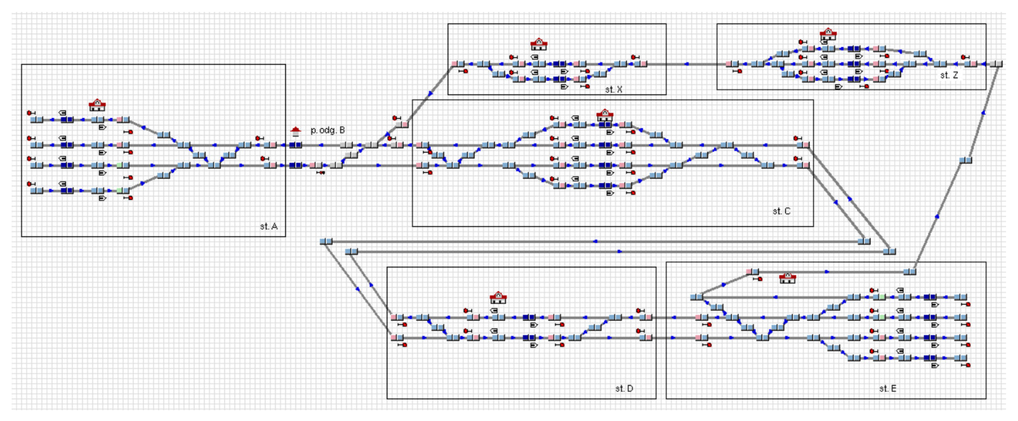
Figure 1. (a) Delay distribution and (b) times between failures (TBF) distribution.
Energies 14 08248 g001
Figure 2. Simulation operation.
Energies 14 08248 g002
Figure 3. Evaluation model.
Energies 14 08248 g003
Figure 4. Model of the analyzed railroad line.
Energies 14 08248 g004
Figure 5. Distribution of train delays: (a) A–B route, (b) B–C route, (c) C–E route, (d) A–Z route, (e) Z–E route.
Energies 14 08248 g005aEnergies 14 08248 g005b
Figure 6. Energy losses due to unscheduled stops for the given steps of the margin adding method.
Energies 14 08248 g006
Table 1. Route parameters.
StationNumber of PlatformsNumber of Tracks
A54
C44
D22
E54
X12
Z22
Table 2. Energy consumption for the analyzed train types.
Train TypeTarget velocityDistance to Reach the Target Velocity from Standstill during Acceleration Time to Get the Target velocity from Standstill during Acceleration Resistance force Under target VelocityEnergy Consumption for One Acceleration from Standstill to the Target VelocityEnergy Consumption for Movement with Constant Velocity (Target Velocity)Increased Energy Consumption per One Acceleration from Standstill to the Target Velocity
(km/h)(km)(min)(kN)(kWh)(kWh)(kWh)
Electric multiple unit 45We1201.170.9314.8037.384.8132.57
EU07 locomotive with 6 passenger coaches2.722.0330.5089.6823.0466.64
Table 3. Results after all iterations for both directions on each section.
SectionCurrent Reserve (min)Delay for 95% (min)Reserve 0 (min)Delay for 95% (min)Reserve I Step (min)Delay for 95% (min)Reserve II Step (min)Delay for 95% (min)Reserve III Step
(min)
Delay for 95% (min)Reserve IV Step (min)Delay for 95% (min)
A–B2.530120.571.552.5331.5
B–C340111.572.553441.5
C–E530111.563.544.545.51.5
A–Z52.509.5262.554.535.52
Z–E3.5309.5253.55444.52
Table 4. The average number of unscheduled train stops per 12 h of stimulation combined with the energy loss.
ReserveExpress TrainRegio Train
No. of Unscheduled Stops Energy Loss (MWh)No. of Unscheduled Stops Energy Loss (MWh)
current reserve method211.40240.79
reserve 01177.801264.10
reserve I step825.46933.03
reserve II step312.07381.24
reserve III step151.00180.59
reserve IV step60.4080.26
Publisher’s Note: MDPI stays neutral with regard to jurisdictional claims in published maps and institutional affiliations.

