
Position Estimation at Zero Speed for PMSMs Using Artificial Neural Networks


Abstract
1. Introduction
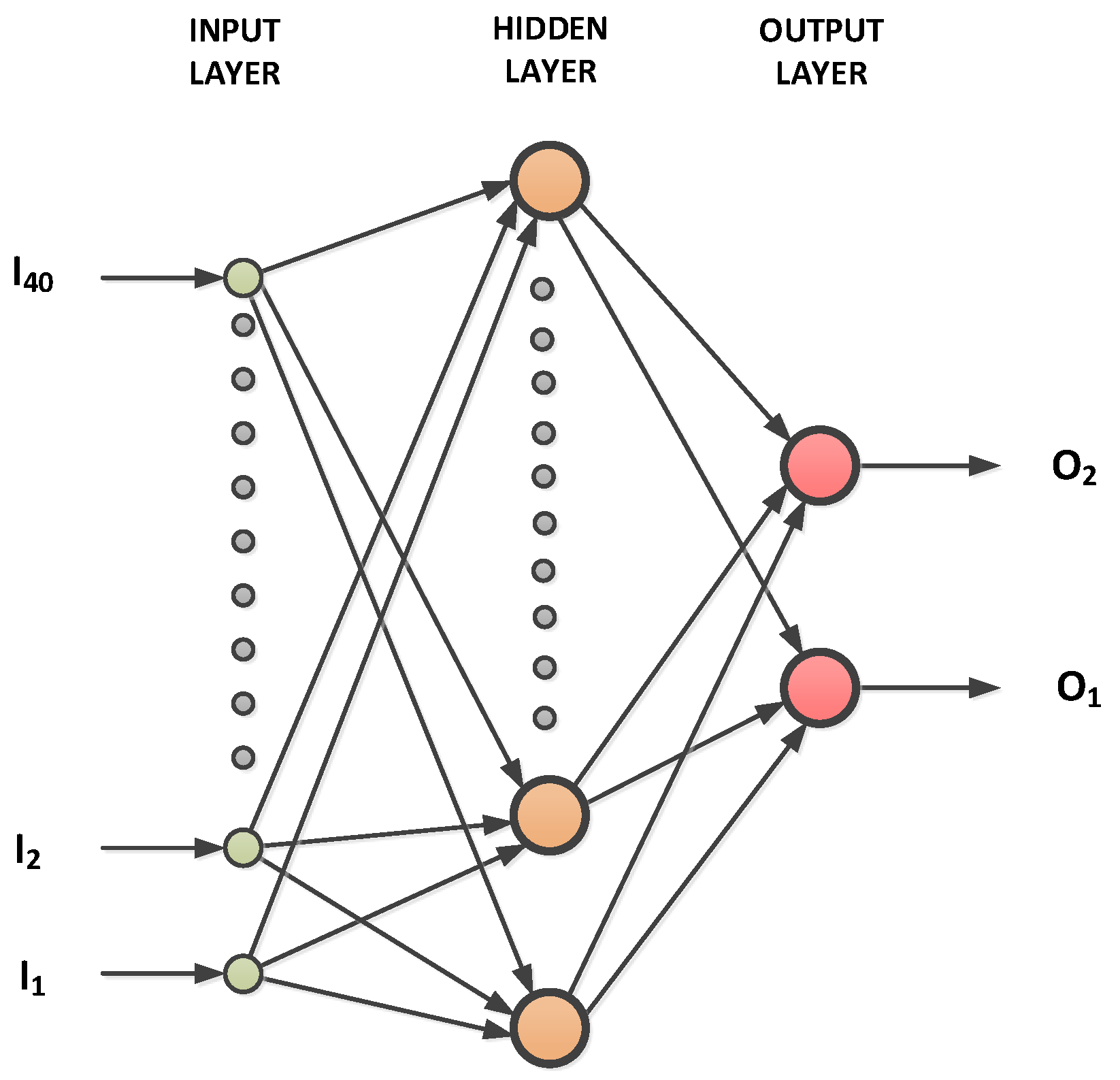
- The current hodograph is processed as a point in a multi-dimensional space and not as a 2D image.
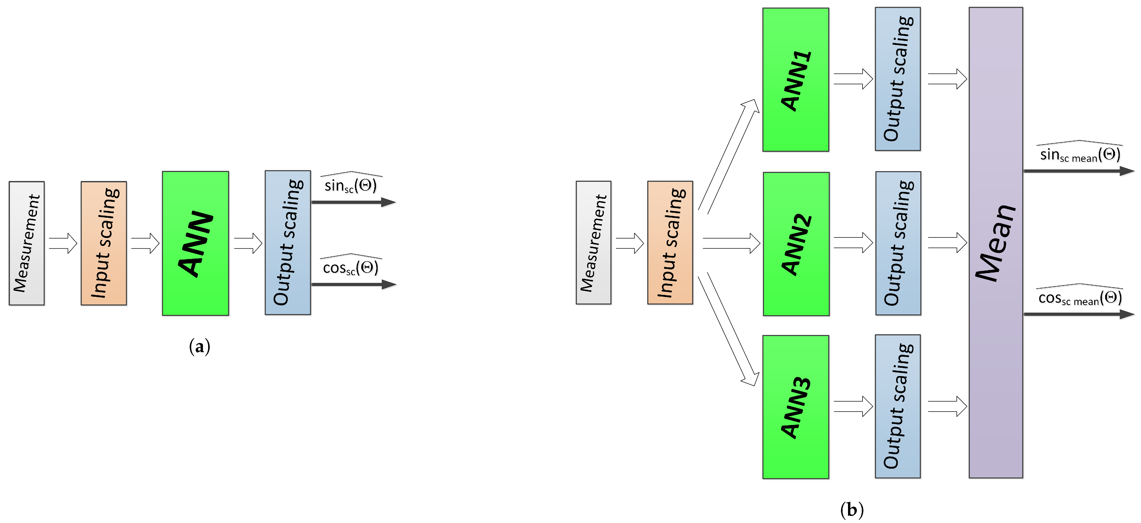
- Several small, unidirectional, shallow artificial neural networks acting on common data were used.
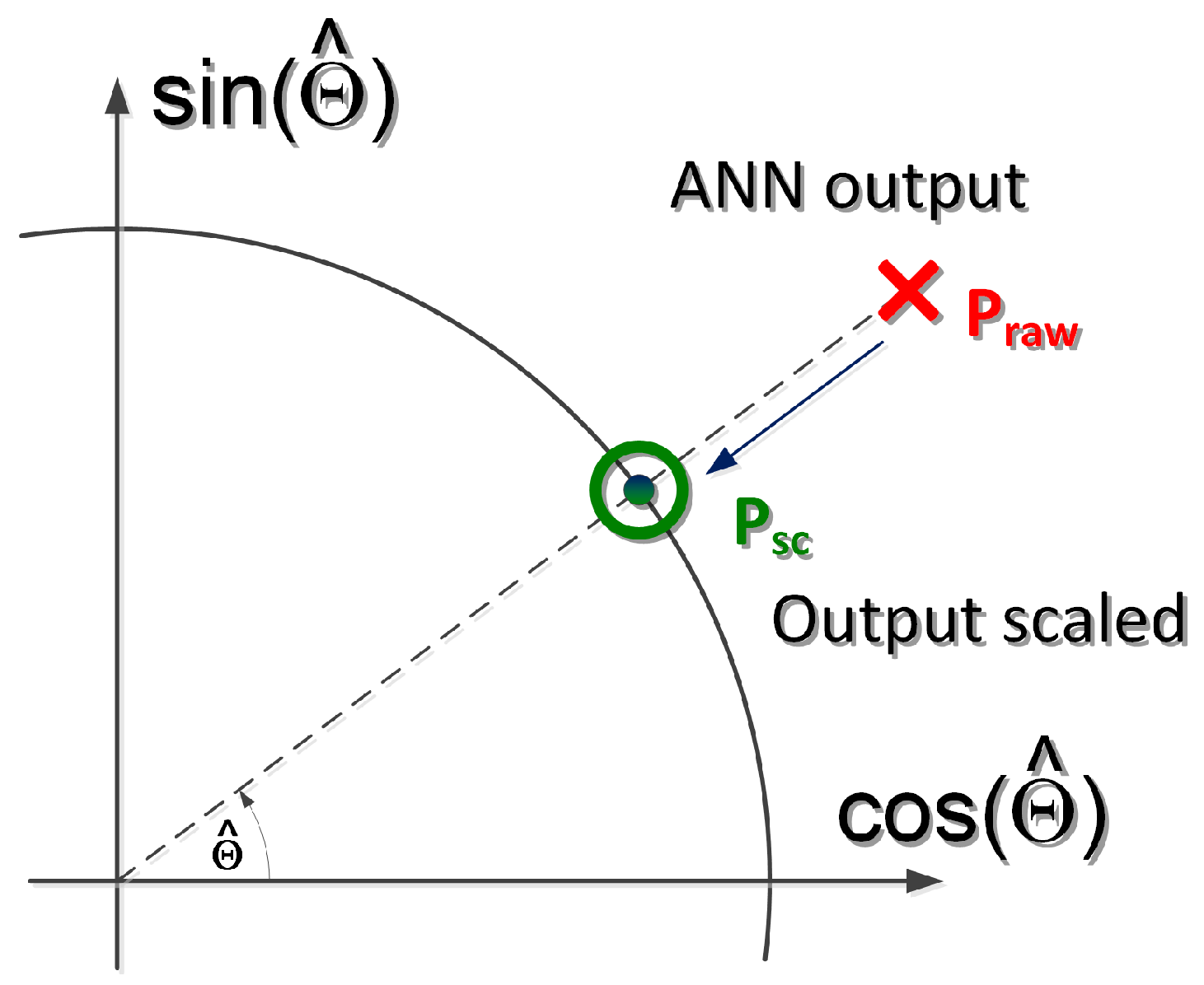
- The output of the ANNs are scaled.
- The results of the individual networks are aggregated to produce a final value.
2. Model of a PMSM
3. Position Estimation
3.1. The Estimation Concept
3.2. The Estimator
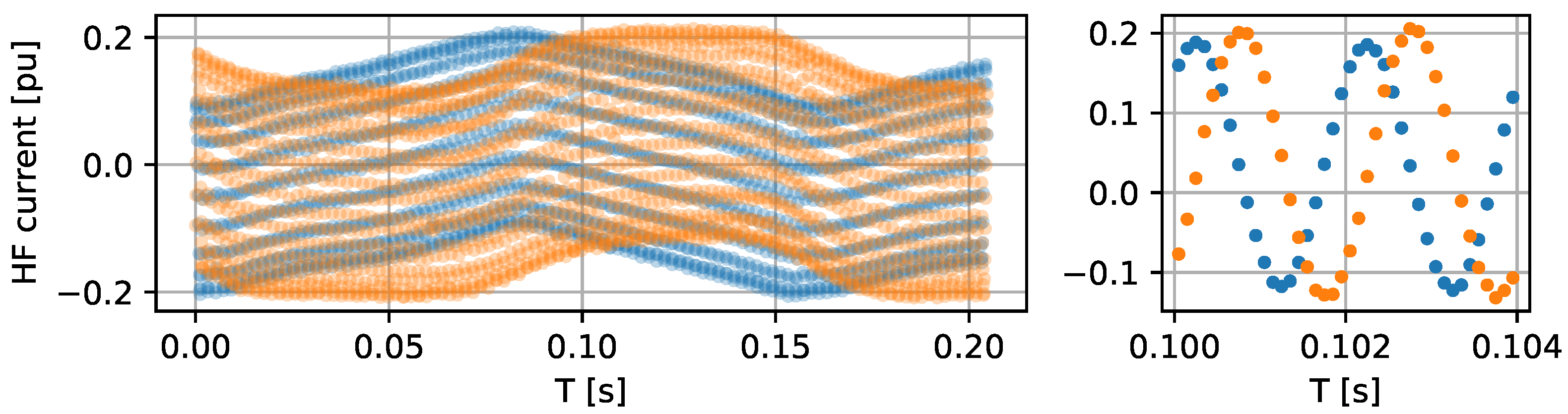
- Recording of high-frequency currents.
- Centering and scaling of the current hodograph.
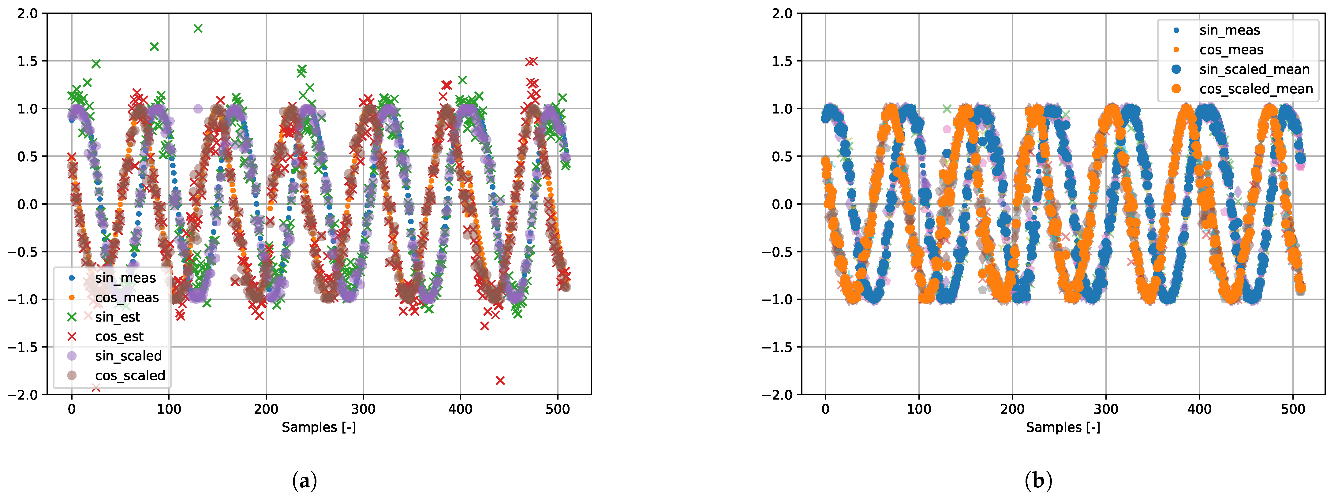
- Computing the ANN output (sine and cosine of estimated position).
- Scaling the ANN output.
- Improving the estimation.
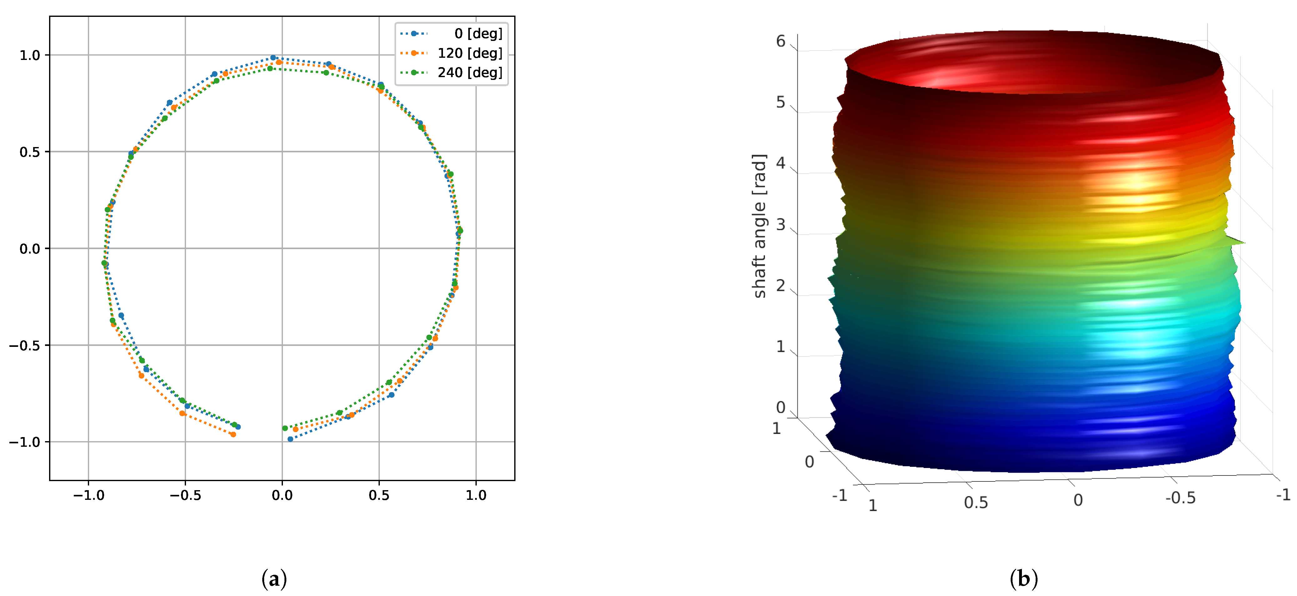
3.3. Recording of High-Frequency Currents
3.4. Centering and Scaling of the Current Hodograph
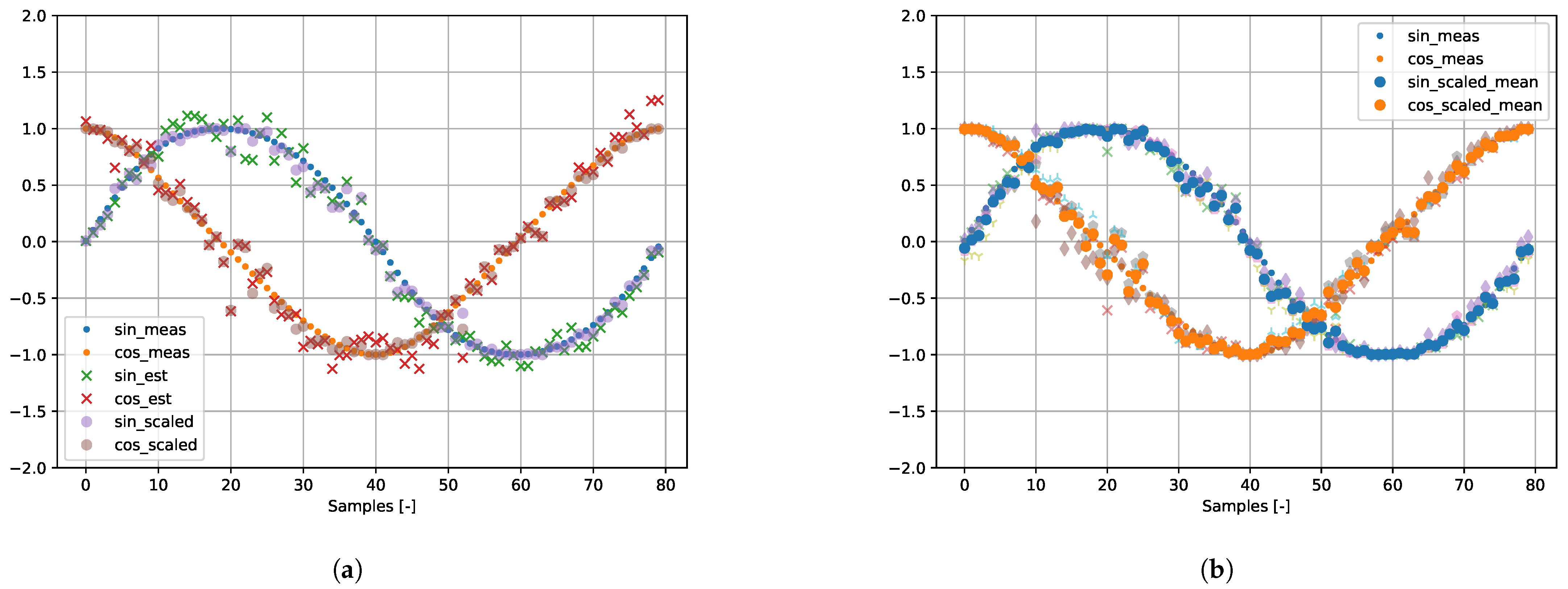
3.5. Computing the ANN Output
| model = Sequential() |
| model.add(Dense(neurons_1W, input_dim = (2 ∗ data_length), |
| activation = ‘sigmoid’)) |
| model.add(Dense(2)). |
3.6. Scaling the ANN Output
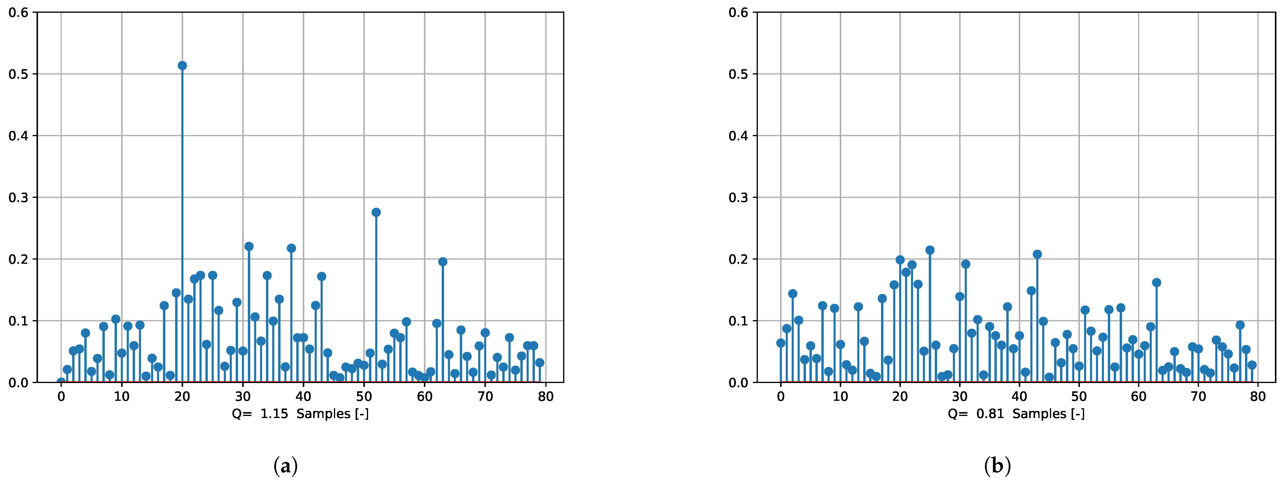
3.7. Improving the Estimation
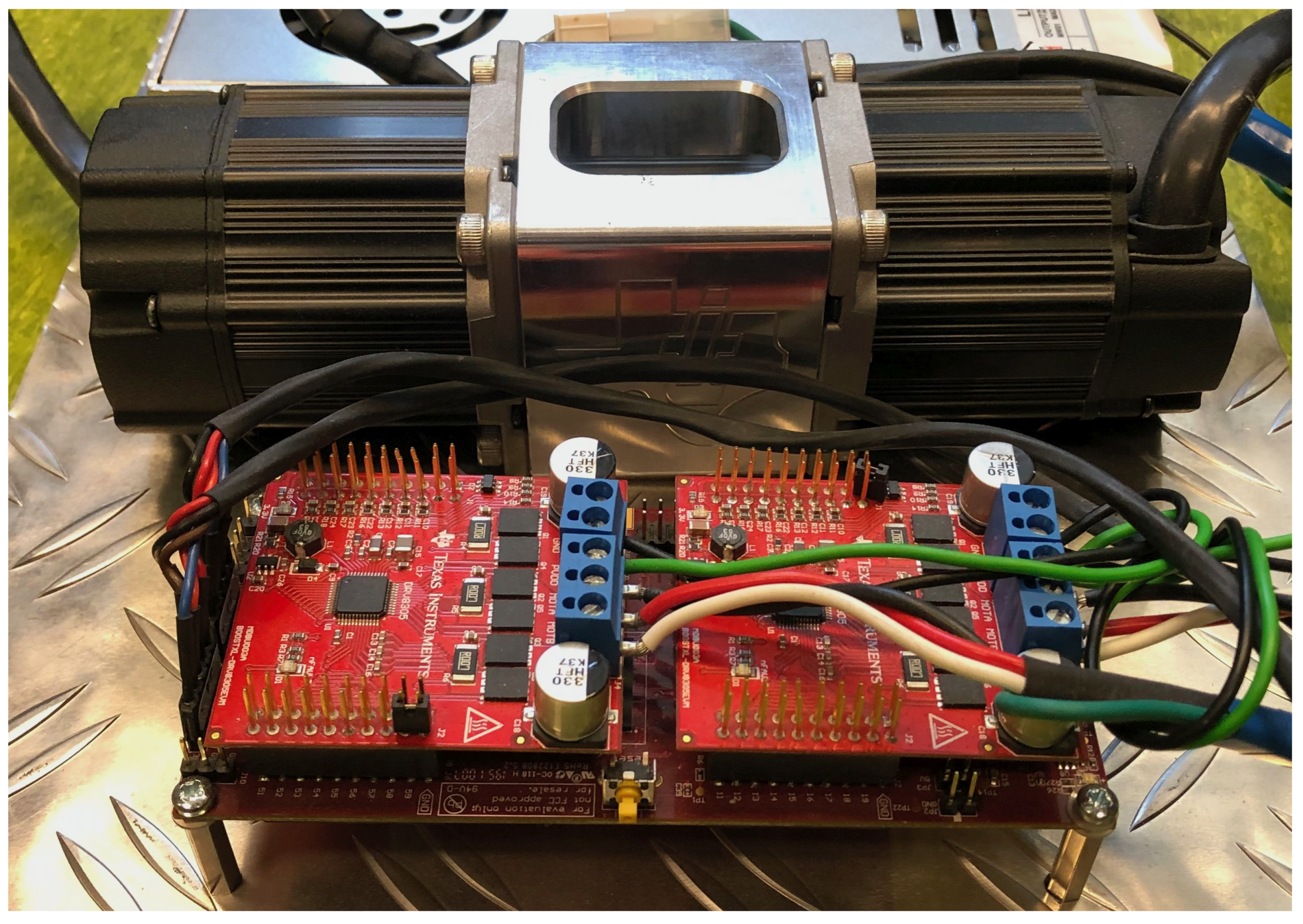
4. Laboratory Stand
- .
5. Results
5.1. Input Data
5.2. ANN Calculation
big_set#2 = set#10 + set#9 + ,..., + set#1
6. Conclusions
Author Contributions
Funding
Conflicts of Interest
Abbreviations
| ANN | Artificial Neural Network |
| BEMF | Back Electromotive Force |
| BPF | Band-Pass Filter |
| BSF | Band-Stop Filter |
| FOC | Field-Oriented Control |
| PMSM | Permanent Magnet Synchronous Motor |
References
- Liu, K.; Zhang, Q.; Chen, J.; Zhu, Z.Q.; Zhang, J. Online Multiparameter Estimation of Nonsalient-Pole PM Synchronous Machines With Temperature Variation Tracking. IEEE Trans. Ind. Electron. 2011, 58, 1776–1788. [Google Scholar] [CrossRef]
- Moreau, S.; Kahoul, R.; Louis, J.P. Parameters estimation of permanent magnet synchronous machine without adding extra-signal as input excitation. In Proceedings of the Industrial Electronics, 2004 IEEE International Symposium on IEEE, Ajaccio, France, 4–7 May 2004; Volume 1, pp. 371–376. [Google Scholar]
- Parasiliti, F.; Petrella, R.; Tursini, M. Sensorless Speed Control of a PM Synchronous Motor Based on Sliding Mode Observer and Extended Kalman Filter; IEEE: Chicago, IL, USA, 2001; Volume 1, pp. 533–540. [Google Scholar] [CrossRef]
- Baek, S.W.; Lee, S.W. Design Optimization and Experimental Verification of Permanent Magnet Synchronous Motor Used in Electric Compressors in Electric Vehicles. Appl. Sci. 2020, 10, 3235. [Google Scholar] [CrossRef]
- Qiu, Z.; Chen, Y.; Lin, X.; Cheng, H.; Kang, Y.; Liu, X. Hybrid Carrier Frequency Modulation Based on Rotor Position to Reduce Sideband Vibro-Acoustics in PMSM Used by Electric Vehicles. World Electr. Veh. J. 2021, 12, 100. [Google Scholar] [CrossRef]
- Łebkowski, A. Design, Analysis of the Location and Materials of Neodymium Magnets on the Torque and Power of In-Wheel External Rotor PMSM for Electric Vehicles. Energies 2018, 11, 2293. [Google Scholar] [CrossRef]
- Gao, H.; Zhang, W.; Wang, Y.; Chen, Z. Fault-Tolerant Control Strategy for 12-Phase Permanent Magnet Synchronous Motor. Energies 2019, 12, 3462. [Google Scholar] [CrossRef]
- Hezzi, A.; Ben Elghali, S.; Bensalem, Y.; Zhou, Z.; Benbouzid, M.; Abdelkrim, M.N. ADRC-Based Robust and Resilient Control of a 5-Phase PMSM Driven Electric Vehicle. Machines 2020, 8, 17. [Google Scholar] [CrossRef]
- Wisniewski, J.; Koczara, W. Control of Axial Flux Permanent Magnet Motor by the PIPCRM method at standstill and at low speed. In Proceedings of the Power Electronics and Motion Control Conference, EPE-PEMC 2008, 13th, Poznań, Poland, 1–3 September 2008; pp. 2254–2260. [Google Scholar]
- Janiszewski, D. Load Torque Estimation for sensorless PMSM drive with output filter fed by PWM converter. In Proceedings of the 39th Annual Conference of the IEEE Industrial Electronics Society (IECON 2013), Vienna, Austria, 10–13 November 2013; pp. 2953–2959. [Google Scholar]
- Seilmeier, M.; Ebersberger, S.; Piepenbreier, B. PMSM model for sensorless control considering saturation induced secondary saliencies. In Proceedings of the 2013 IEEE International Symposium on Sensorless Control for Electrical Drives and Predictive Control of Electrical Drives and Power Electronics (SLED/PRECEDE), Munich, Germany, 17–19 October 2013; pp. 1–8. [Google Scholar] [CrossRef]
- Quang, N.; Ha, Q.; Hieu, N. FPGA sensorless PMSM drive with adaptive fading extended Kalman filtering. In Proceedings of the 2014 13th International Conference on Control Automation Robotics Vision (ICARCV), Singapore, 10–12 December 2014; pp. 295–300. [Google Scholar] [CrossRef]
- Fernandes, E.; Oliveira, A.; Vitorino, M.; dos Santos, E.; Santos, W. Speed sensorless PMSM motor drive system based on four-switch three-phase converter. In Proceedings of the IECON 2014—40th Annual Conference of the IEEE Industrial Electronics Society, Dallas, TX, USA, 29 October–1 November 2014; pp. 902–906. [Google Scholar] [CrossRef]
- Xu, P.; Zhu, Z. Analysis of carrier signal injection based sensorless control of PMSM drives under limited inverter switching frequency condition. In Proceedings of the 2014 IEEE Energy Conversion Congress and Exposition (ECCE), Pittsburgh, PA, USA, 14–18 September 2014; pp. 4131–4138. [Google Scholar] [CrossRef]
- Benevieri, A.; Marchesoni, M.; Passalacqua, M.; Vaccaro, L. Experimental Low-Speed Performance Evaluation of Sensorless Passive Algorithms for SPMSM. IEEE Trans. Energy Convers. 2021. [Google Scholar] [CrossRef]
- Yoo, J.; Sul, S.K. Stability Analysis of PI-Controller-Type Position Estimator for Sensorless PMSM Drives in Flux Weakening Region. In Proceedings of the 2021 IEEE Transportation Electrification Conference & Expo (ITEC), Chicago, IL, USA, 21–25 June 2021; pp. 434–438. [Google Scholar] [CrossRef]
- Wang, Z.; Lu, Q.; Ye, Y.; Lu, K.; Fang, Y. Investigation of PMSM Back-EMF Using Sensorless Control with Parameter Variations and Measurement Errors. Prz. Elektrotech. 2012, 88, 182–186. [Google Scholar]
- Hamida, M.; De Leon, J.; Glumineau, A.; Boisliveau, R. An Adaptive Interconnected Observer for Sensorless Control of PM Synchronous Motors With Online Parameter Identification. IEEE Trans. Ind. Electron. 2013, 60, 739–748. [Google Scholar] [CrossRef]
- Nair, S.V.; Hatua, K.; Prasad, N.V.P.R.D.; Reddy, D.K. A Quick I-f Starting of PMSM Drive With Pole Slipping Prevention and Reduced Speed Oscillations. IEEE Trans. Ind. Electron. 2021, 68, 6650–6661. [Google Scholar] [CrossRef]
- Corley, M.J.; Lorenz, R.D. Rotor position and velocity estimation for a salient-pole permanent magnet synchronous machine at standstill and high speeds. IEEE Trans. Ind. Appl. 1998, 34, 784–789. [Google Scholar] [CrossRef]
- Schroedl, M. Sensorless control of AC machines at low speed and standstill based on the “INFORM” method. In Proceedings of the Conference Record of the 1996 IEEE Industry Applications Conference, Thirty-First IAS Annual Meeting, IAS ’96, San Diego, CA, USA, 6–10 October 1996; Volume 1, pp. 270–277. [Google Scholar] [CrossRef]
- Zentai, A.; Daboczi, T. Improving INFORM calculation method on permanent magnet synchronous machines. In Proceedings of the IEEE Instrumentation and Measurement Technology Conference Proceedings, IMTC 2007, Warsaw, Poland, 1–3 May 2007; pp. 1–6. [Google Scholar] [CrossRef]
- Scicluna, K.; Staines, C.S.; Raute, R. Sensorless Low/Zero Speed Estimation for Permanent Magnet Synchronous Machine Using a Search-Based Real-Time Commissioning Method. IEEE Trans. Ind. Electron. 2020, 67, 6010–6018. [Google Scholar] [CrossRef]
- Abry, F.; Zgorski, A.; Lin-Shi, X.; Retif, J.M. Sensorless position control for SPMSM at zero speed and acceleration. In Proceedings of the 2011—14th European Conference on Power Electronics and Applications (EPE 2011), Birmingham, UK, 30 August–1 September 2011; pp. 1–9. [Google Scholar]
- Pando-Acedo, J.; Romero-Cadaval, E.; Milanes-Montero, M.I.; Barrero-Gonzalez, F. Improvements on a Sensorless Scheme for a Surface-Mounted Permanent Magnet Synchronous Motor Using Very Low Voltage Injection. Energies 2020, 13, 2732. [Google Scholar] [CrossRef]
- Ilioudis, V.C. Sensorless Control of Permanent Magnet Synchronous Machine with Magnetic Saliency Tracking Based on Voltage Signal Injection. Machines 2020, 8, 14. [Google Scholar] [CrossRef]
- Pillay, P.; Krishnan, R. Modeling, simulation, and analysis of permanent-magnet motor drives. I. The permanent-magnet synchronous motor drive. IEEE Trans. Ind. Appl. 1989, 25, 265–273. [Google Scholar] [CrossRef]
- Szabat, K.; Wróbel, K.; Dróżdż, K.; Janiszewski, D.; Pajchrowski, T.; Wójcik, A. A Fuzzy Unscented Kalman Filter in the Adaptive Control System of a Drive System with a Flexible Joint. Energies 2020, 13, 2056. [Google Scholar] [CrossRef]
- Urbanski, K.; Janiszewski, D. Sensorless Control of the Permanent Magnet Synchronous Motor. Sensors 2019, 19, 3546. [Google Scholar] [CrossRef]
- Nicola, M.; Nicola, C.I. Sensorless Fractional Order Control of PMSM Based on Synergetic and Sliding Mode Controllers. Electronics 2020, 9, 1494. [Google Scholar] [CrossRef]
- Vas, P. Sensorless Vector and Direct Torque Control; Number 42 in Monographs in Electrical and Electronic Engineering; Oxford University Press: Oxford, UK; New York, NY, USA, 1998. [Google Scholar]
- Malinowski, M.; Kazmierkowski, M.; Trzynadlowski, A. A comparative study of control techniques for PWM rectifiers in AC adjustable speed drives. IEEE Trans. Power Electron. 2003, 18, 1390–1396. [Google Scholar] [CrossRef]
- Brock, S. Analysis and Simulation of Electrical and Computer Systems; Chapter Robust Integral Sliding Mode Tracking Control of a Servo Drives with Reference Trajectory Generator; Springer International Publishing: Cham, Switzerland, 2015; pp. 305–313. [Google Scholar] [CrossRef]
- Kazmierkowski, M.; Franquelo, L.; Rodriguez, J.; Perez, M.; Leon, J. High-Performance Motor Drives. IEEE Ind. Electron. Mag. 2011, 5, 6–26. [Google Scholar] [CrossRef]
- Urbanski, K.; Majchrzak, D. Faults detection in PMSM drive using Artificial Neural Network. Prz. Elektrotech. 2017, 1, 22–25. [Google Scholar] [CrossRef][Green Version]
- Sinha, A.K.; Kumar, P.; Hati, A.S. ANN Based Fault Detection Scheme for Bearing Condition Monitoring in SRIMs using FFT, DWT and Band-pass Filters. In Proceedings of the 2020 International Conference on Power, Instrumentation, Control and Computing (PICC), Thrissur, India, 17–19 December 2020; pp. 1–6. [Google Scholar] [CrossRef]
- Li, S.; Won, H.; Fu, X.; Fairbank, M.; Wunsch, D.C.; Alonso, E. Neural-Network Vector Controller for Permanent-Magnet Synchronous Motor Drives: Simulated and Hardware-Validated Results. IEEE Trans. Cybern. 2020, 50, 3218–3230. [Google Scholar] [CrossRef]
- Yao, C.; Sun, Z.; Xu, S.; Zhang, H.; Ren, G.; Ma, G. Optimal Parameters Design for Model Predictive Control using an Artificial Neural Network Optimized by Genetic Algorithm. In Proceedings of the 2021 13th International Symposium on Linear Drives for Industry Applications (LDIA), Wuhan, China, 1–3 July 2021; pp. 1–6. [Google Scholar] [CrossRef]
- Ramírez-Cárdenas, O.D.; Trujillo-Romero, F. Sensorless Speed Tracking of a Brushless DC Motor Using a Neural Network. Math. Comput. Appl. 2020, 25, 57. [Google Scholar] [CrossRef]
- Urbanski, K. Position Estimation at Zero Speed for PMSM Using Probabilistic Neural Network. In Proceedings of the 2015 IEEE 2nd International Conference on Cybernetics (Cybconf), Gdynia, Poland, 24–26 June 2015; pp. 427–432. [Google Scholar]
- Park, G.; Kim, G.; Gu, B.G. Sensorless PMSM Drive Inductance Estimation Based on a Data-Driven Approach. Electronics 2021, 10, 791. [Google Scholar] [CrossRef]


| ANN#1 | ANN#2 | ANN#3 | ANN#4 | Multi-ANN | |
|---|---|---|---|---|---|
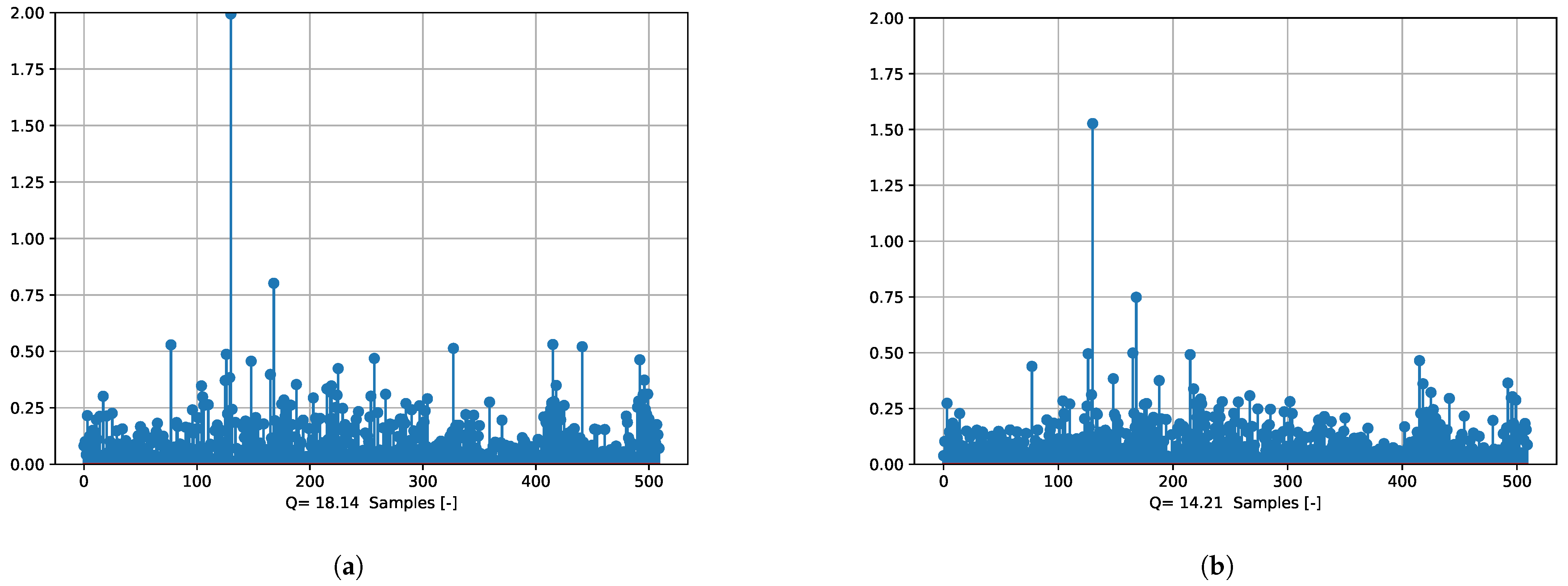
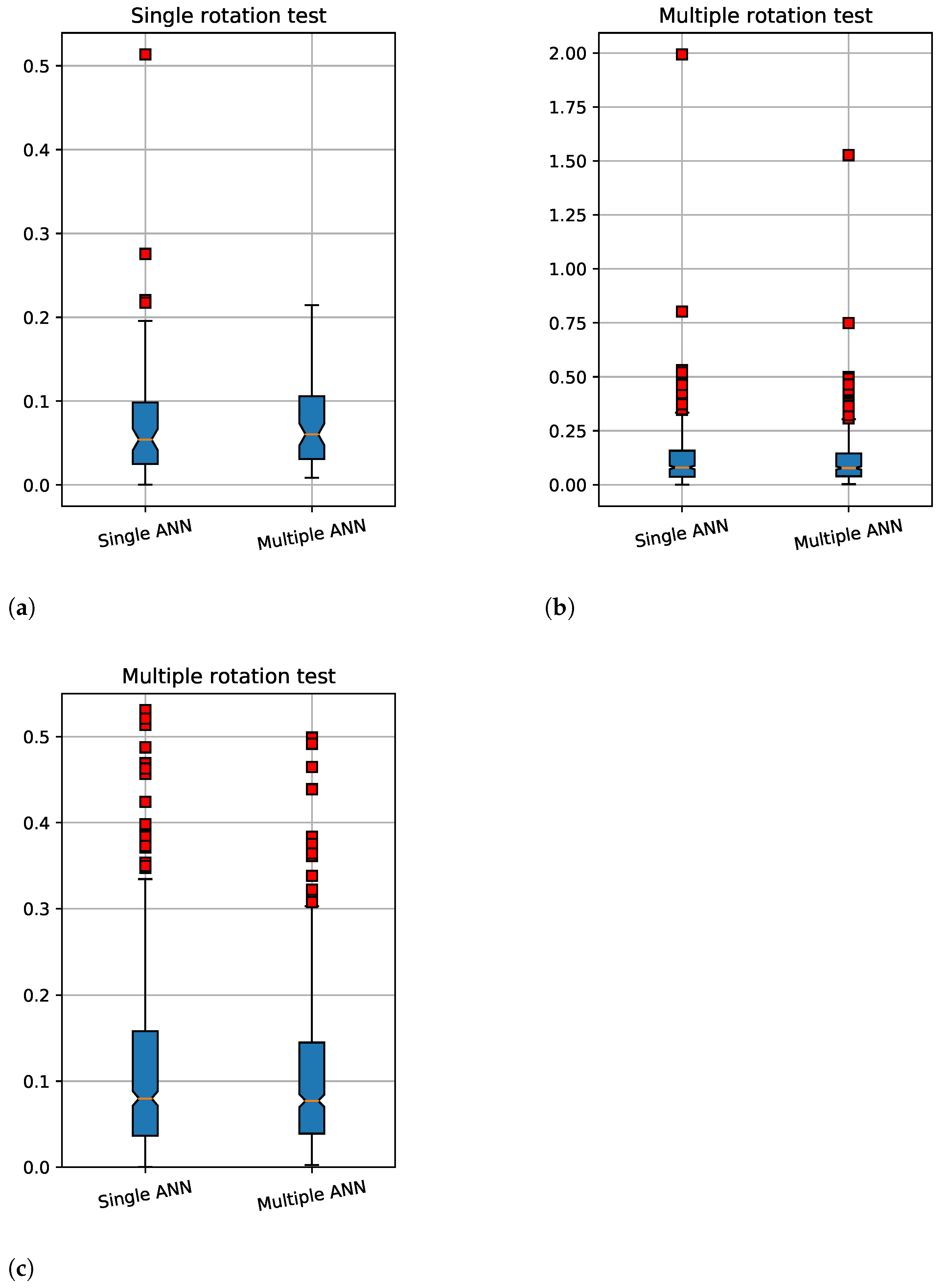
| Quality index | 18.1 | 19.2 | 17.2 | 18.8 | 14.2 |
| Max. error | 2 | 1.05 | 1.78 | 1.44 | 1.52 |
Publisher’s Note: MDPI stays neutral with regard to jurisdictional claims in published maps and institutional affiliations. |
© 2021 by the authors. Licensee MDPI, Basel, Switzerland. This article is an open access article distributed under the terms and conditions of the Creative Commons Attribution (CC BY) license (https://creativecommons.org/licenses/by/4.0/).
Share and Cite
Urbanski, K.; Janiszewski, D. Position Estimation at Zero Speed for PMSMs Using Artificial Neural Networks. Energies 2021, 14, 8134. https://doi.org/10.3390/en14238134
Urbanski K, Janiszewski D. Position Estimation at Zero Speed for PMSMs Using Artificial Neural Networks. Energies. 2021; 14(23):8134. https://doi.org/10.3390/en14238134
Chicago/Turabian StyleUrbanski, Konrad, and Dariusz Janiszewski. 2021. "Position Estimation at Zero Speed for PMSMs Using Artificial Neural Networks" Energies 14, no. 23: 8134. https://doi.org/10.3390/en14238134
APA StyleUrbanski, K., & Janiszewski, D. (2021). Position Estimation at Zero Speed for PMSMs Using Artificial Neural Networks. Energies, 14(23), 8134. https://doi.org/10.3390/en14238134