
A Comparative Study on Fuel Consumption Prediction Methods of Heavy-Duty Diesel Trucks Considering 21 Influencing Factors


Abstract
:1. Introduction
1.1. Background
1.2. Literature Review
1.2.1. Research on Factors Influencing Fuel Consumption
1.2.2. Research on Fuel Consumption Model
1.2.3. Research on Fleet Management System
1.3. Research Objectives and Innovation
2. Data and Method
2.1. Data
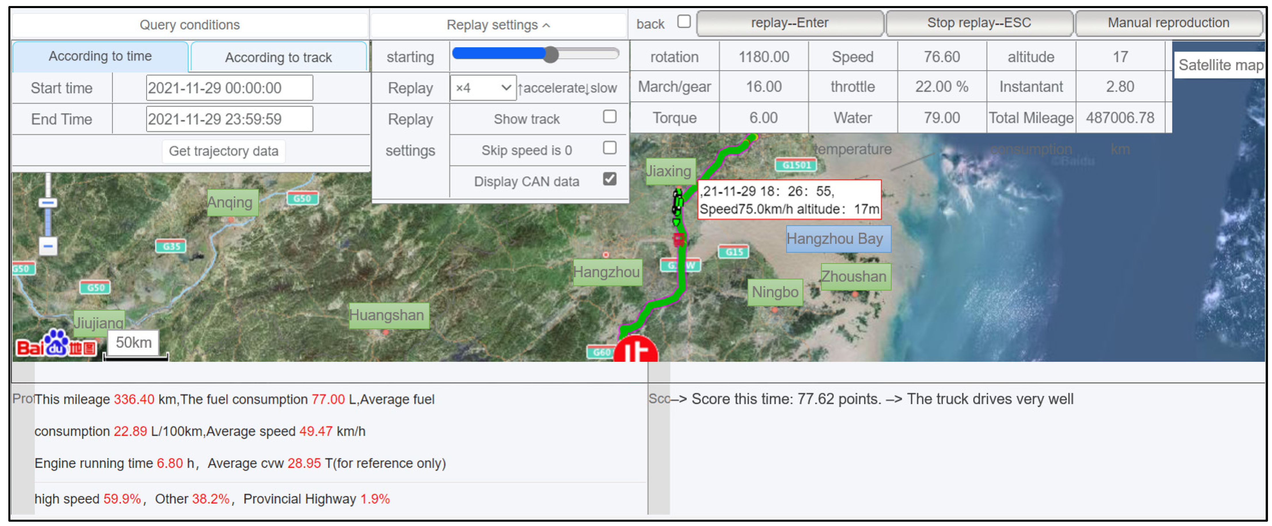
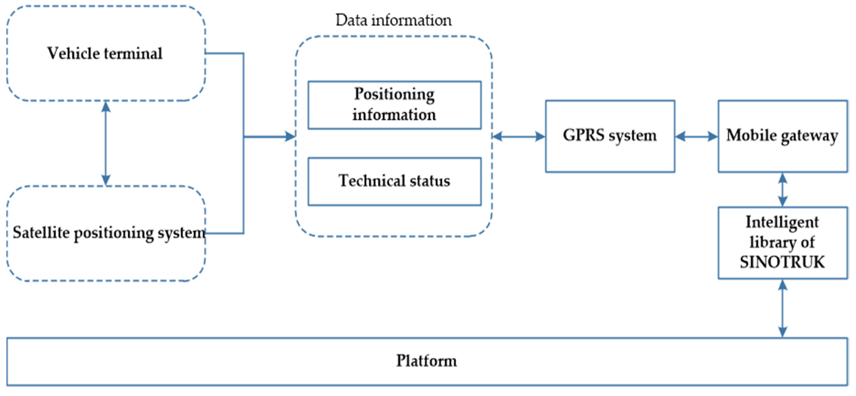
2.1.1. Data Source
2.1.2. Data Processing
- (1)
- Specific data types
- (2)
- Data standardization
- (3)
- Data summary statistics
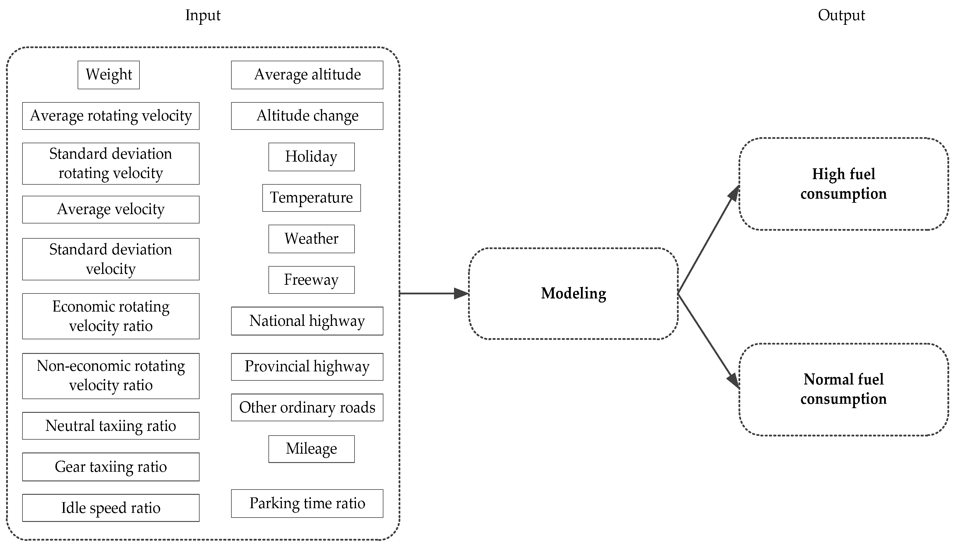
2.2. Methodology
2.2.1. Binary Logistic Regression
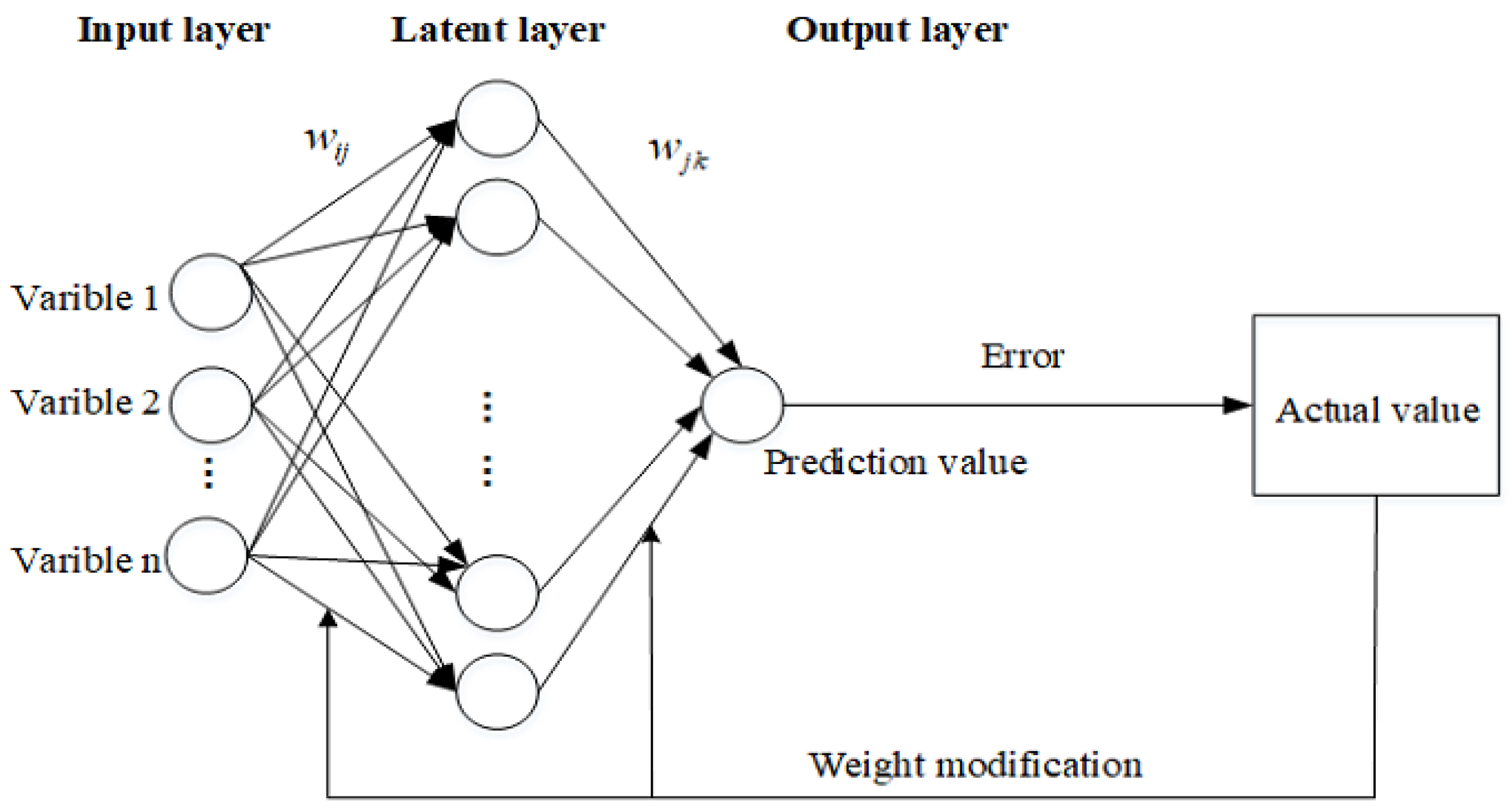
2.2.2. BP Neural Network
2.2.3. Decision Tree
2.2.4. Random Forest
3. Modeling Results and Discussions
3.1. Binary Logistic Regression Model
- (1)
- Collinearity diagnosis of variables
- (2)
- Binary Logistic regression model
3.2. Machine Learning
3.2.1. Model Training
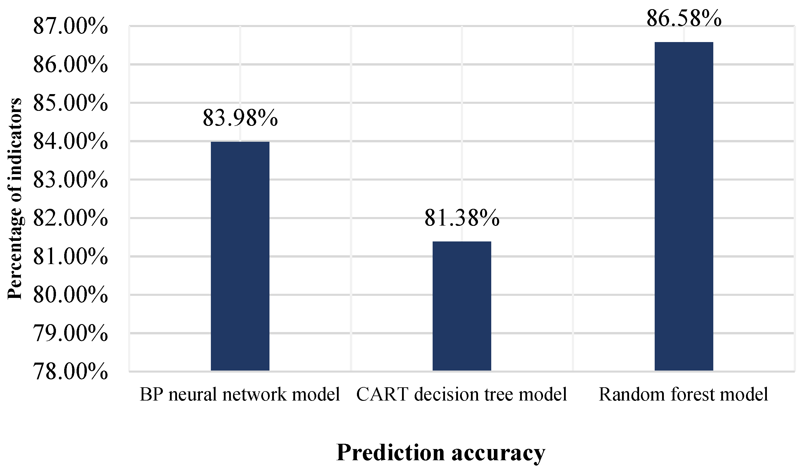
3.2.2. Model Results and Comparison Analysis
4. Conclusions
Author Contributions
Funding
Institutional Review Board Statement
Informed Consent Statement
Data Availability Statement
Acknowledgments
Conflicts of Interest
References
- Guensler, R.; Liu, H.; Xu, Y.; Akanser, A.; Kim, D.; Hunter, M.P.; Rodgers, M.O. Energy consumption and emissions modeling of individual vehicles. Transp. Res. Rec. 2017, 2627, 93–102. [Google Scholar] [CrossRef]
- Ahn, K.; Rakha, H.; Trani, A.; Van Aerde, M. Estimating vehicle fuel consumption and emissions based on instantaneous speed and acceleration levels. J. Transp. Eng. 2002, 128, 182–190. [Google Scholar] [CrossRef]
- Hlasny, T.; Fanti, M.P.; Mangini, A.M.; Rotunno, G.; Turchiano, B. Optimal fuel consumption for heavy trucks: A review. In Proceedings of the 2017 IEEE International Conference on Service Operations and Logistics, and Informatics (SOLI 2017), Bari, Italy, 18–20 September 2017; pp. 80–85. [Google Scholar] [CrossRef]
- Li, D.; Li, C.; Miwa, T.; Morikawa, T. An exploration of factors affecting drivers’ daily fuel consumption efficiencies considering multi-level random effects. Sustainability 2019, 11, 393. [Google Scholar] [CrossRef] [Green Version]
- Chen, Y.; Zhu, L.; Gonder, J.; Young, S.; Walkowicz, K. Data-driven fuel consumption estimation: A multivariate adaptive regression spline approach. Transp. Res. Part C Emerg. Technol. 2017, 83, 134–145. [Google Scholar] [CrossRef]
- Ericsson, E. Independent driving pattern factors and their influence on fuel-use and exhaust emission factors. Transp. Res. Part D Transp. Environ. 2001, 6, 325–345. [Google Scholar] [CrossRef]
- Zhou, M.; Jin, H.; Wang, W. A review of vehicle fuel consumption models to evaluate eco-driving and eco-routing. Transp. Res. Part D Transp. Environ. 2016, 49, 203–218. [Google Scholar] [CrossRef]
- Cachón, L.; Pucher, E. Fuel Consumption Simulation Model of a CNG Vehicle based on Real-world Emission Measurement. SAE Tech. Pap. 2007, 24, 114–123. [Google Scholar] [CrossRef]
- Wang, H.; Fu, L.; Zhou, Y.; Li, H. Modelling of the fuel consumption for passenger cars regarding driving characteristics. Transp. Res. Part D Transp. Environ. 2008, 13, 479–482. [Google Scholar] [CrossRef]
- Xiang, Y.; Li, Z.; Chen, M.Y.; Jiang, X.M. Research on calculation software of fuel consumption for heavy trucks. In Proceedings of the 3rd International Conference on Measuring Technology and Mechatronics Automation (ICMTMA 2011), Shanghai, China, 6–7 January 2011; Volume 2, pp. 1121–1124. [Google Scholar] [CrossRef]
- Wang, J.; Rakha, H.A. Fuel consumption model for heavy duty diesel trucks: Model development and testing. Transp. Res. Part D Transp. Environ. 2017, 55, 127–141. [Google Scholar] [CrossRef]
- Ma, H.; Xie, H.; Chen, S.; Yan, Y.; Huang, D. Effects of driver acceleration behavior on fuel consumption of city buses. SAE Tech. Pap. 2014, 1, 389–395. [Google Scholar] [CrossRef]
- Du, Y.; Wu, J.; Yang, S.; Zhou, L. Predicting vehicle fuel consumption patterns using floating vehicle data. J. Environ. Sci. 2017, 59, 24–29. [Google Scholar] [CrossRef] [PubMed]
- Wysocki, O.; Deka, L.; Elizondo, D. Heavy Duty Vehicle Fuel Consumption Modelling Using Artificial Neural Networks. In Proceedings of the 25th International Conference on Automation and Computing (ICAC), Lancaster, UK, 5–7 September 2019; pp. 1–6. [Google Scholar] [CrossRef]
- Mane, A.; Djordjevic, B.; Ghosh, B. A data-driven framework for incentivising fuel-efficient driving behaviour in heavy-duty vehicles. Transp. Res. Part D Transp. Environ. 2021, 95, 102845. [Google Scholar] [CrossRef]
- Walnum, H.J.; Simonsen, M. Does driving behavior matter? An analysis of fuel consumption data from heavy-duty trucks. Transp. Res. Part D Transp. Environ. 2015, 36, 107–120. [Google Scholar] [CrossRef]
- Toledo, G.; Shiftan, Y. Can feedback from in-vehicle data recorders improve driver behavior and reduce fuel consumption? Transp. Res. Part A Policy Pract. 2016, 94, 194–204. [Google Scholar] [CrossRef]
- Sun, R.; Chen, Y.; Dubey, A.; Pugliese, P. Hybrid electric buses fuel consumption prediction based on real-world driving data. Transp. Res. Part D Transp. Environ. 2021, 91, 102637. [Google Scholar] [CrossRef]
- Guo, D.; Wang, J.; Zhao, J.B.; Sun, F.; Gao, S.; Li, C.D.; Li, M.H.; Li, C.C. A vehicle path planning method based on a dynamic traffic network that considers fuel consumption and emissions. Sci. Total Environ. 2019, 663, 935–943. [Google Scholar] [CrossRef] [PubMed]
- Faria, M.V.; Duarte, G.O.; Varella, R.A.; Farias, T.L.; Baptista, P.C. How do road grade, road type and driving aggressiveness impact vehicle fuel consumption? Assessing potential fuel savings in Lisbon, Portugal. Transp. Res. Part D Transp. Environ. 2019, 72, 148–161. [Google Scholar] [CrossRef]
- Lee, S. Application of logistic regression model and its validation for landslide susceptibility mapping using GIS and remote sensing data. Int. J. Remote Sens. 2005, 26, 1477–1491. [Google Scholar] [CrossRef]
- Ozdemir, A. Using a binary logistic regression method and GIS for evaluating and mapping the groundwater spring potential in the Sultan Mountains (Aksehir, Turkey). J. Hydrol. 2011, 405, 123–136. [Google Scholar] [CrossRef]
- Zhang, Z.; Wang, C. The Research of Vehicle Plate Recognition Technical Based on BP Neural Network. AASRI Procedia 2012, 1, 74–81. [Google Scholar] [CrossRef]
- Ma, J.; Li, D.; Lu, Y.; Chen, J. Intelligent Diagnosis System for Vehicle Network Based on BP Neural Network. IOP Conf. Ser. Mater. Sci. Eng. 2018, 452, 42004. [Google Scholar] [CrossRef]
- Yao, Y.; Zhao, X.; Liu, C.; Rong, J.; Zhang, Y.; Dong, Z.; Su, Y.; Chen, F. Vehicle Fuel Consumption Prediction Method Based on Driving Behavior Data Collected from Smartphones. J. Adv. Transp. 2020, 2020, 9263605. [Google Scholar] [CrossRef]
- Li, H.; Dong, H.; Jia, L.; Ren, M. Vehicle classification with single multi-functional magnetic sensor and optimal MNS-based CART. Meas. J. Int. Meas. Confed. 2014, 55, 142–152. [Google Scholar] [CrossRef]
- Zeng, L.; Guo, J.; Wang, B.; Lv, J.; Wang, Q. Analyzing sustainability of Chinese coal cities using a decision tree modeling approach. Resour. Policy 2019, 64, 101501. [Google Scholar] [CrossRef]
- Breiman, L. Random forests. Mach. Learn. 2001, 45, 5–32. [Google Scholar] [CrossRef] [Green Version]
- Zhang, X.; Zhang, J.; Zhang, J.; Zhang, Y. Research on the Combined Prediction Model of Residential Building Energy Consumption Based on Random Forest and BP Neural Network. Geofluids 2021, 2021, 7271383. [Google Scholar] [CrossRef]
- Li, L.H.; Zhu, J.S.; Shan, X.H.; Zhang, X. Prediction modeling of railway short-term passenger flow based on random forest regression. In Lecture Notes in Electrical Engineering; Springer: Singapore, 2019; Volume 503. [Google Scholar] [CrossRef]
- Wang, Y.; Zhang, J.; Liu, P.; Xu, C.; Zhang, F. Identification of Non-Green Channel Vehicles at Highway Toll Gate Based on Logistic Regression Model. In Proceedings of the 19th COTA International Conference of Transportation Professionals, Nanjing, China, 6–8 July 2019. [Google Scholar] [CrossRef]
- Schendera, C.F. Regressionsanalyse Mit SPSS; De Gruyter Oldenbourg: Berlin, Germany, 2014. [Google Scholar]
- Peng, Y.; Peng, S.; Wang, X.; Tan, S. An investigation on fatality of drivers in vehicle–fixed object accidents on expressways in China: Using multinomial logistic regression model. Proc. Inst. Mech. Eng. Part H J. Eng. Med. 2018, 232, 643–654. [Google Scholar] [CrossRef] [PubMed]
- Zargarnezhad, S.; Dashti, R.; Ahmadi, R. Predicting vehicle fuel consumption in energy distribution companies using ANNs. Transp. Res. Part D Transp. Environ. 2019, 74, 174–188. [Google Scholar] [CrossRef]
- Dobre, A. Theoretical Study Regarding the Fuel Consumption Performance for a Vehicle Equipped with a Mechanical Transmission. Procedia Manuf. 2019, 32, 537–544. [Google Scholar] [CrossRef]
- Zhou, X.; Huang, J.; Lv, W.; Li, D. Fuel consumption estimates based on driving pattern recognition. In Proceedings of the 2013 IEEE International Conference on Green Computing and Communications and IEEE Internet of Things and IEEE Cyber, Physical and Social Computing, Beijing, China, 20–23 August 2013; pp. 496–503. [Google Scholar] [CrossRef]
- Hao, C.; Ge, Y.; Wang, X. Heavy-duty diesel engine fuel consumption comparison with diesel and biodiesel measured at different altitudes. Int. J. Veh. Perform. 2020, 6, 263–276. [Google Scholar] [CrossRef]
- Jeon, H. The impact of climate change on passenger vehicle fuel consumption: Evidence from U.S. panel data. Energies 2019, 12, 4460. [Google Scholar] [CrossRef] [Green Version]
- Soni, A.R.; Chandel, M.K. Impact of rainfall on travel time and fuel usage for Greater Mumbai city. Transp. Res. Procedia 2020, 48, 2096–2107. [Google Scholar] [CrossRef]
- He, J.; Qi, Z.; Hang, W.; Zhao, C.; King, M. Predicting freeway pavement construction cost using a back-propagation neural network: A case study in Henan, China. Baltic J. Road Bridge Eng. 2014, 9, 66–76. [Google Scholar] [CrossRef]
- Lantz, B. Machine Learning with R, 2nd ed.; Packt Publishing: Birmingham, UK, 2015. [Google Scholar]
- Trigila, A.; Iadanza, C.; Esposito, C.; Scarascia-Mugnozza, G. Comparison of Logistic Regression and Random Forests techniques for shallow landslide susceptibility assessment in Giampilieri (NE Sicily, Italy). Geomorphology 2015, 249, 119–136. [Google Scholar] [CrossRef]
- Zhou, X.; Lu, P.; Zheng, Z.; Tolliver, D.; Keramati, A. Accident Prediction Accuracy Assessment for Highway-Rail Grade Crossings Using Random Forest Algorithm Compared with Decision Tree. Reliab. Eng. Syst. Saf. 2020, 200, 106931. [Google Scholar] [CrossRef]


| Factors | Source | |
|---|---|---|
| Vehicle-related | Engine technical state | [6] |
| Driving system technical state | ||
| Transmission system technical state | ||
| Environment-related | Average altitude | [7] |
| Temperature | ||
| Humidity | ||
| Wind | ||
| Weather conditions | ||
| Driving-related | Long-term driving styles | [7] |
| Long-term driving habits | ||
| Going qualifications | ||
| Driving styles influenced by weather and date | ||
| Road-related | Road features | [8] |
| Road geometry |
| Parameter Type | Parameter Value | Parameter Type | Parameter Value |
|---|---|---|---|
| Drive form | 4X2 or 6X2R | Vehicle weight | 8.54 tons |
| Engine | Sinotruk MC13.54-50 | Total mass | 25 tons |
| Maximum horsepower | 540 horsepower | Fuel type | diesel |
| Emission standards | National five | Number of passengers | 3 people |
| Gearbox | ZF16S2530 TO | Displacement | 12.419 L |
| Discrete Data Name | Classification Description | Standardized Value |
|---|---|---|
| Holiday | Yes | 1 |
| No | 0 | |
| Temperature | Under 10 °C | 0 |
| 11–15 °C | 1 | |
| 16–20 °C | 2 | |
| 21–25 °C | 3 | |
| 25–30 °C | 4 | |
| More than 30 °C | 5 | |
| Weather | No rain | 0 |
| Precipitation 1–8 mm | 1 | |
| Precipitation 10–20 mm | 2 | |
| Fuel consumption per 100 km | Normal fuel consumption | 0 |
| High fuel consumption | 1 |
| Variable Name (Type) | Definition |
|---|---|
| Driving Characteristics | |
| Neutral taxiing ratio(continuous) | Percentage of truck driving time with no engine load during a trip |
| Gear taxiing ratio(continuous) | Percentage of truck driving time with engine load during a trip |
| Idle speed ratio(continuous) | Percentage of time spent idling during a trip |
| Parking time ratio(continuous) | Percentage of time spent parking during a trip |
| Environment Characteristics | |
| Average altitude(continuous) | Average altitude per trip/(100 m) |
| Altitude change(continuous) | The change of altitude per trip/(100 m) |
| Holiday(discrete) | A discrete variable indicating whether the driving day is a holiday |
| Temperature(discrete) | A discrete variable indicating outdoor temperature while driving |
| Weather(discrete) | A discrete variable indicating weather while driving, expressed in precipitation in this paper |
| Vehicle Characteristics | |
| Weight(continuous) | Average cargo weight per trip/(ton) |
| Average rotating velocity(continuous) | Average engine rotating velocity per trip/(100 r/min) |
| Standard deviation rotating velocity(continuous) | The standard deviation of engine rotating velocity per trip |
| Average velocity(continuous) | Average speed per trip/(km/h) |
| Standard deviation velocity(continuous) | The standard deviation of speed per trip |
| Economic rotating velocity ratio(continuous) | Percentage of truck driving time in the economic rotating velocity range during a trip |
| Non-economic rotating velocity ratio(continuous) | Percentage of truck driving time in the non-economic rotating velocity range during a trip |
| Road Characteristics | |
| Freeway(continuous) | Percentage of distance the truck travels on freeways during a trip |
| National road(continuous) | Percentage of distance the truck travels on ordinary national roads during a trip |
| Provincial road(continuous) | Percentage of distance the truck travels on ordinary provincial roads during a trip |
| Other ordinary roads(continuous) | Percentage of distance the truck travels on other low-grade roads during a trip |
| Mileage(continuous) | Mileage during a trip |
| Fuel consumption(discrete) | Fuel consumption per hundred kilometers for each trip |
| VIF | 1/VIF | VIF | 1/VIF | ||
|---|---|---|---|---|---|
| Weight | 2.845 | 0.352 | Idle speed ratio | 90,579.430 | 0.000 |
| Freeway | 991.271 | 0.001 | Non-economic rotating velocity ratio | 87,492.734 | 0.000 |
| National road | 264.490 | 0.004 | Parking time ratio | 602,7043.000 | 0.000 |
| Provincial road | 315.954 | 0.003 | Average altitude | 2.781 | 0.360 |
| Other ordinary roads | 535.602 | 0.002 | Altitude change | 3.331 | 0.300 |
| Mileage | 39.075 | 0.026 | 1.Holiday | 1.103 | 0.906 |
| Average rotating velocity | 4.521 | 0.221 | 1.Temperature | 1.998 | 0.501 |
| Standard deviation rotating velocity | 5.499 | 0.182 | 2.Temperature | 1.996 | 0.501 |
| Average velocity | 5.751 | 0.174 | 3.Temperature | 1.707 | 0.586 |
| Standard deviation velocity | 3.366 | 0.297 | 4.Temperature | 1.425 | 0.702 |
| Economic rotating velocity ratio | 4,832,594.500 | 0.000 | 5.Temperature | 1.119 | 0.894 |
| Neutral taxiing ratio | 16,775.566 | 0.000 | 1.Weather | 1.104 | 0.905 |
| Gear taxiing ratio | 7721.713 | 0.000 | 2.Weather | 1.039 | 0.962 |
| Mean VIF | 425,553.600 | ||||
| Fuel Consumption | Coef. | St.Err. | t-Value | p-Value | 95% Conf | Interval | Sig |
|---|---|---|---|---|---|---|---|
| Weight | 1.617 | 0.055 | 14.020 | 0.000 | 1.512 | 1.730 | *** |
| Average rotating velocity | 0.989 | 0.002 | −6.320 | 0.000 | 0.985 | 0.992 | *** |
| Standard deviation rotating velocity | 0.984 | 0.005 | −3.410 | 0.001 | 0.975 | 0.993 | *** |
| Average velocity | 0.769 | 0.017 | −11.780 | 0.000 | 0.736 | 0.803 | *** |
| Standard deviation velocity | 0.887 | 0.034 | −3.130 | 0.002 | 0.823 | 0.956 | *** |
| Average altitude | 1.002 | 0.001 | 2.700 | 0.007 | 1.001 | 1.004 | *** |
| Altitude change | 0.999 | 0.000 | −1.330 | 0.184 | 0.998 | 1.000 | |
| 0.Holiday | base | ||||||
| 1.Holiday | 0.923 | 0.586 | −0.130 | 0.900 | 0.266 | 3.206 | |
| 0.Temperature | base | ||||||
| 1.Temperature | 0.796 | 0.212 | −0.860 | 0.392 | 0.473 | 1.341 | |
| 2.Temperature | 1.000 | 0.291 | −0.000 | 1.000 | 0.566 | 1.768 | |
| 3.Temperature | 1.777 | 0.603 | 1.700 | 0.090 | 0.914 | 3.455 | * |
| 4.Temperature | 1.240 | 0.605 | 0.440 | 0.659 | 0.477 | 3.227 | |
| 5.Temperature | 18.100 | 14.03 | 3.740 | 0.000 | 3.962 | 82.698 | *** |
| 0.Weather | base | ||||||
| 1.Weather | 0.552 | 0.154 | −2.130 | 0.033 | 0.320 | 0.954 | ** |
| 2.Weather | 0.935 | 0.931 | −0.070 | 0.946 | 0.133 | 6.587 | |
| Constant | 1,184,552.6 | 2,242,029.9 | 7.39 | 0 | 29,004.515 | 48,377,460 | *** |
| Variables | Odds Ratio | Std.Err. | z | p > z | 95% Conf. | Interval |
|---|---|---|---|---|---|---|
| Weight | 0.046 | 0.004 | 12.640 | 0.000 *** | 0.039 | 0.054 |
| Average rotating velocity | −0.001 | 0.000 | −6.200 | 0.000 *** | −0.001 | −0.001 |
| Standard deviation rotating velocity | −0.002 | 0.000 | −3.420 | 0.001 *** | −0.002 | −0.001 |
| Average velocity | −0.025 | 0.002 | −11.000 | 0.000 *** | −0.030 | −0.021 |
| Standard deviation velocity | −0.012 | 0.004 | −3.060 | 0.002 *** | −0.019 | −0.004 |
| Average altitude | 0.001 | 0.000 | 2.700 | 0.007 *** | 0.000 | 0.000 |
| Altitude change | −0.000 | 0.000 | −1.320 | 0.187 | −0.000 | 0.000 |
| 1.Holiday | −0.007 | 0.058 | −0.130 | 0.897 | −0.121 | 0.106 |
| 1.Temperature | −0.019 | 0.023 | −0.830 | 0.405 | −0.065 | 0.026 |
| 2.Temperature | −0.000 | 0.027 | 0.000 | 1.000 | −0.053 | 0.053 |
| 3.Temperature | 0.067 | 0.042 | 1.600 | 0.111 | −0.015 | 0.149 |
| 4.Temperature | 0.022 | 0.052 | 0.420 | 0.675 | −0.080 | 0.123 |
| 5.Temperature | 0.573 | 0.163 | 3.510 | 0.000 *** | 0.253 | 0.892 |
| 1.Weather | −0.049 | 0.020 | −2.480 | 0.013 ** | −0.088 | −0.010 |
| 2.Weather | −0.007 | 0.098 | −0.070 | 0.944 | −0.200 | 0.186 |
| Number | cp | nsplit | rel Error | xerror | xstd |
|---|---|---|---|---|---|
| 1 | 0.064677 | 0 | 1.00000 | 1.00000 | 0.062374 |
| 2 | 0.044776 | 3 | 0.80597 | 0.93035 | 0.060744 |
| 3 | 0.024876 | 4 | 0.76119 | 0.95025 | 0.061223 |
| 4 | 0.018242 | 6 | 0.71144 | 0.92537 | 0.060623 |
| 5 | 0.014925 | 12 | 0.58209 | 0.92783 | 0.060822 |
| 6 | 0.010000 | 15 | 0.53731 | 0.93532 | 0.060865 |
Publisher’s Note: MDPI stays neutral with regard to jurisdictional claims in published maps and institutional affiliations. |
© 2021 by the authors. Licensee MDPI, Basel, Switzerland. This article is an open access article distributed under the terms and conditions of the Creative Commons Attribution (CC BY) license (https://creativecommons.org/licenses/by/4.0/).
Share and Cite
Gong, J.; Shang, J.; Li, L.; Zhang, C.; He, J.; Ma, J. A Comparative Study on Fuel Consumption Prediction Methods of Heavy-Duty Diesel Trucks Considering 21 Influencing Factors. Energies 2021, 14, 8106. https://doi.org/10.3390/en14238106
Gong J, Shang J, Li L, Zhang C, He J, Ma J. A Comparative Study on Fuel Consumption Prediction Methods of Heavy-Duty Diesel Trucks Considering 21 Influencing Factors. Energies. 2021; 14(23):8106. https://doi.org/10.3390/en14238106
Chicago/Turabian StyleGong, Jian, Junzhu Shang, Lei Li, Changjian Zhang, Jie He, and Jinhang Ma. 2021. "A Comparative Study on Fuel Consumption Prediction Methods of Heavy-Duty Diesel Trucks Considering 21 Influencing Factors" Energies 14, no. 23: 8106. https://doi.org/10.3390/en14238106
APA StyleGong, J., Shang, J., Li, L., Zhang, C., He, J., & Ma, J. (2021). A Comparative Study on Fuel Consumption Prediction Methods of Heavy-Duty Diesel Trucks Considering 21 Influencing Factors. Energies, 14(23), 8106. https://doi.org/10.3390/en14238106